How cost-effective are new cancer drugs in the U.S.?

ABSTRACT

Introduction

More than 8 times as many new cancer drugs were approved during 2005–2015 as were approved during 1975–1985 (66 vs. 8). The average annual 2010–2014 growth rate of U.S. cancer drug expenditure was 7.6%. This has contributed to a lively debate about the value and cost-effectiveness of new cancer drugs.

Areas covered

We assess the average cost-effectiveness in the U.S. in 2014 of new cancer drugs approved by the FDA during 2000–2014, by performing an original econometric investigation (rather than a literature review) of whether there were larger declines in premature mortality and hospitalization, and larger increases in survival, from the cancers that had larger increases in the number of drugs ever approved, controlling for the change in cancer incidence and mean age at time of diagnosis.

Expert opinion

Cancer drugs approved during 2000–2014 are estimated to have reduced the number of potential years of life lost before age 75 in 2014 by 719,133. Cancer drugs approved during 1989–2005 are estimated to have reduced hospital cost in 2013 by $4.8 billion. Our baseline estimate of the cost per life-year gained in 2014 from cancer drugs approved during 2000–2014 is $7853.

KEYWORDS:

• Cancer
• cost-effectiveness
• hospitalization
• innovation
• longevity
• mortality
• survival

1. Introduction

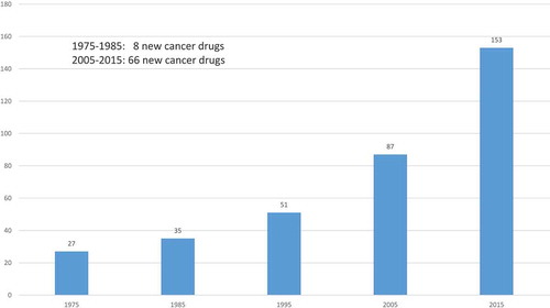
The number of drugs approved by the Food and Drug Administration (FDA) for treating cancer has increased substantially during the last 40 years. As shown in Figure 1, 27 drugs for treating cancer had been approved by the FDA by 1975; that number increased to 153 by 2015. Moreover, cancer drug innovation has been accelerating: more than 8 times as many new cancer drugs were approved during 2005–2015 as were approved during 1975–1985 (66 vs. 8). In contrast, as shown in Figure A1, the number of ‘non-cancer’ drugs launched worldwide has tended to decline.

Figure 1. Number of drugs used to treat cancer ever approved by the FDA.

The rapid growth in the number of drugs for treating cancer has been accompanied by a substantial increase in expenditure on cancer drugs. Data on U.S. sales during 2010–2014 of all cancer drugs and of the 10 largest selling (in 2014) drugs are shown in Table A1. The average annual growth rate of total expenditure was 7.6%–more than 3.6 times the average annual growth rate of nominal U.S. GDP. This has contributed to a lively debate about the value and cost-effectiveness of new cancer drugs.

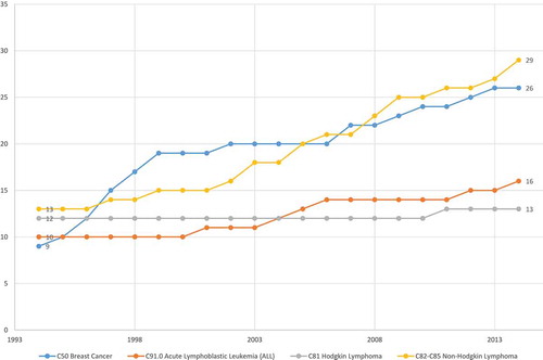
In this population-based observational research study, we will attempt to assess the average cost-effectiveness in the U.S. in 2014 of the drugs that the FDA approved for treating cancer during the period 2000–2014. Cost-effectiveness will be measured as the ratio of the impact of new cancer drugs on medical expenditure to their impact on potential years of life lost (PYLL) due to cancer.¹ Our study design will exploit the fact that, while the overall number of drugs for treating cancer has increased, data from the National Cancer Institute (NCI) and the FDA indicate that the size of the increase varied considerably across cancer sites (breast, colon, lung, etc.). The NCI publishes lists of drugs approved for 39 different types of cancer [1].² The first year in which each drug was first approved by the FDA can be determined from the Drugs@FDA database [2]. By combining data from these two sources, we can measure the history of pharmaceutical innovation for each type of cancer. This is illustrated by Figure 2, which shows data on drugs that have been approved by the FDA for the treatment of one type of cancer, acute lymphoblastic leukemia. During the period 1994–2014, the number of drugs ever approved for acute lymphoblastic leukemia increased from 10 to 16. Figure 3 shows the number of drugs ever approved during the same period for four types of cancer. A similar number of (between 9 and 13) drugs had ever been approved for each of the four types in 1994. During the next 20 years, 16 new drugs for non-Hodgkin lymphoma and 17 new drugs for breast cancer were approved, but only 6 new drugs for acute lymphoblastic leukemia and one new drug for Hodgkin lymphoma were approved.

Figure 2. Drugs approved for Acute Lymphoblastic Leukemia.

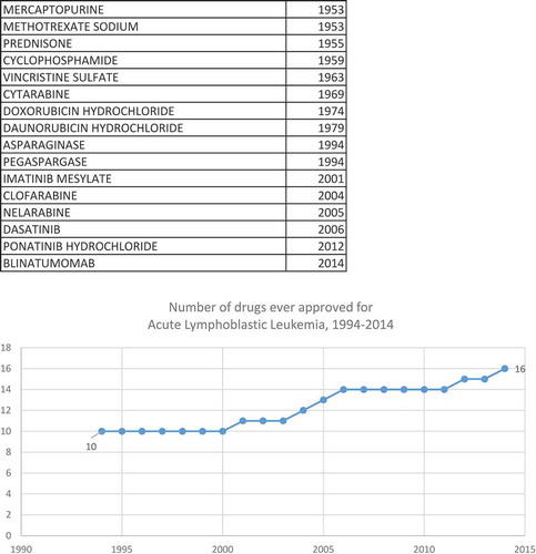
Figure 3. Number of drugs ever approved for 4 types of cancer, 1994–2014.

To estimate the impact of the drugs approved during the period 2000–2014 on PYLL (‘premature mortality’) due to cancer in 2014, we will estimate difference-in-differences models using longitudinal data on the cancer sites defined by the National Cancer Institute [1]. In essence, we will investigate whether there were larger declines in mortality from the cancers that had larger increases in the number of drugs ever approved, controlling for the change in cancer incidence and mean age at time of diagnosis.³ We will analyze two alternative measures of premature mortality: potential years of life lost before ages 75 and 65. In addition, we will analyze the impact of the number of drugs approved on the 5-year observed survival rate, also controlling for the expected survival rate of non-cancer patients. Some of the estimated models will distinguish between the effects of ‘priority-review’ drugs – drugs that the FDA believes demonstrate ‘the potential to provide a significant improvement in the safety or effectiveness of the treatment, diagnosis, or prevention of a serious or life-threatening condition’ – and ‘standard-review’ drugs – drugs that the FDA believes do not demonstrate such potential [3].

The effect of drug approvals on cancer mortality may be subject to a lag, so the lag structure of the relationship will be investigated. As a robustness check, we will also test whether mortality depends on future drug approvals.

To determine the impact of new cancer drugs on medical expenditure, we will also estimate difference-in-differences models of hospital utilization. All of the data used to estimate the models of cancer mortality and hospitalization are produced by U.S. government agencies and are publicly available.

In Section 2.1, we describe econometric models of cancer patient outcomes. The data sources used to construct the data to estimate these models are described in Section 2.2. Empirical results are presented in Section 3. In Section 4, we use the estimates along with other data to produce an estimate of the average cost-effectiveness of new cancer drugs. Section 5 provides a conclusion.

2. Analysis

2.1. Models of premature cancer mortality, survival, and hospitalization

We will estimate models with (functions of) three types of dependent variables: PYLL (before two different age thresholds, 75 and 65), 5-year observed survival rates, and number of hospital days.

2.1.1. Premature cancer mortality model

The basic model of potential years of life lost before age 75⁴ is:

(1) $ln\left(\mathrm{P}\mathrm{Y}\mathrm{L}\mathrm{L}{75}_{\mathrm{s},\mathrm{t}}\right)=\beta \mathrm{N}\mathrm{\_}\mathrm{A}\mathrm{P}\mathrm{P}\mathrm{\_}1948\mathrm{\_}{\mathrm{t}}_{\mathrm{s},\mathrm{t}}+\gamma ln\left(\mathrm{C}\mathrm{A}\mathrm{S}\mathrm{E}{\mathrm{S}}_{\mathrm{s},\mathrm{t}}\right)+\pi \mathrm{A}\mathrm{G}\mathrm{E}\mathrm{\_}\mathrm{D}\mathrm{I}\mathrm{A}{\mathrm{G}}_{\mathrm{s},\mathrm{t}}+{\alpha }_s+{\delta }_t+{\epsilon }_{\mathrm{s},\mathrm{t}}$(1)

where

PYLL75s,t	=	= the number of years of potential life lost before age 75 due to cancer at site s in year t (t = 1999, 2014)
N_APP_1948_ts,t	=	= the number of drugs for cancer at site s approved by the FDA between the end of 1948 and the end of year t5
CASESs,t	=	= the average annual number of people below age 75 diagnosed with cancer at site s in years t-9 to t
AGE_DIAGs,t	=	= the mean age at which people below age 75 were diagnosed with cancer at site s in years t-9 to t
αs	=	= a fixed effect for cancer at site s
δt	=	= a fixed effect for year t

The parameter of primary interest in Equation (1)(1) $ln\left(\mathrm{P}\mathrm{Y}\mathrm{L}\mathrm{L}{75}_{\mathrm{s},\mathrm{t}}\right)=\beta \mathrm{N}\mathrm{\_}\mathrm{A}\mathrm{P}\mathrm{P}\mathrm{\_}1948\mathrm{\_}{\mathrm{t}}_{\mathrm{s},\mathrm{t}}+\gamma ln\left(\mathrm{C}\mathrm{A}\mathrm{S}\mathrm{E}{\mathrm{S}}_{\mathrm{s},\mathrm{t}}\right)+\pi \mathrm{A}\mathrm{G}\mathrm{E}\mathrm{\_}\mathrm{D}\mathrm{I}\mathrm{A}{\mathrm{G}}_{\mathrm{s},\mathrm{t}}+{\alpha }_s+{\delta }_t+{\epsilon }_{\mathrm{s},\mathrm{t}}$(1) , which imposes the property of diminishing marginal productivity of drug approvals, is β, the coefficient on the number of drugs that had been approved by the end of year t. Inclusion of year and cancer-site fixed effects controls for the overall change in premature mortality and for stable between-cancer-site differences in premature mortality. A negative and significant estimate of β in Equation (1)(1) $ln\left(\mathrm{P}\mathrm{Y}\mathrm{L}\mathrm{L}{75}_{\mathrm{s},\mathrm{t}}\right)=\beta \mathrm{N}\mathrm{\_}\mathrm{A}\mathrm{P}\mathrm{P}\mathrm{\_}1948\mathrm{\_}{\mathrm{t}}_{\mathrm{s},\mathrm{t}}+\gamma ln\left(\mathrm{C}\mathrm{A}\mathrm{S}\mathrm{E}{\mathrm{S}}_{\mathrm{s},\mathrm{t}}\right)+\pi \mathrm{A}\mathrm{G}\mathrm{E}\mathrm{\_}\mathrm{D}\mathrm{I}\mathrm{A}{\mathrm{G}}_{\mathrm{s},\mathrm{t}}+{\alpha }_s+{\delta }_t+{\epsilon }_{\mathrm{s},\mathrm{t}}$(1) would signify that cancer sites for which there was more pharmaceutical innovation had larger declines in premature mortality. We also control for the average annual number of people below age 75 diagnosed with cancer at site s in years t-9 to t, and their mean age; an increase in mean age at diagnosis is expected to reduce premature mortality.

The drug measure in Equation (1)(1) $ln\left(\mathrm{P}\mathrm{Y}\mathrm{L}\mathrm{L}{75}_{\mathrm{s},\mathrm{t}}\right)=\beta \mathrm{N}\mathrm{\_}\mathrm{A}\mathrm{P}\mathrm{P}\mathrm{\_}1948\mathrm{\_}{\mathrm{t}}_{\mathrm{s},\mathrm{t}}+\gamma ln\left(\mathrm{C}\mathrm{A}\mathrm{S}\mathrm{E}{\mathrm{S}}_{\mathrm{s},\mathrm{t}}\right)+\pi \mathrm{A}\mathrm{G}\mathrm{E}\mathrm{\_}\mathrm{D}\mathrm{I}\mathrm{A}{\mathrm{G}}_{\mathrm{s},\mathrm{t}}+{\alpha }_s+{\delta }_t+{\epsilon }_{\mathrm{s},\mathrm{t}}$(1) is the number of drugs previously approved for a cancer site. The approval of a drug indicates that patients could have been treated with that drug, not necessarily that patients were treated with that drug. We would prefer to estimate models in which the explanatory variables measured the drugs actually used to treat patients, by cancer site and year. Although data are available on the total use of new cancer drugs, many cancer drugs are used for several types of cancer (44% are used to treat 2 or more types of cancer, and 20% are used to treat 3 or more types of cancer), and data on the use of cancer drugs for each type of cancer are not available.

We would also prefer to include in Equation (1)(1) $ln\left(\mathrm{P}\mathrm{Y}\mathrm{L}\mathrm{L}{75}_{\mathrm{s},\mathrm{t}}\right)=\beta \mathrm{N}\mathrm{\_}\mathrm{A}\mathrm{P}\mathrm{P}\mathrm{\_}1948\mathrm{\_}{\mathrm{t}}_{\mathrm{s},\mathrm{t}}+\gamma ln\left(\mathrm{C}\mathrm{A}\mathrm{S}\mathrm{E}{\mathrm{S}}_{\mathrm{s},\mathrm{t}}\right)+\pi \mathrm{A}\mathrm{G}\mathrm{E}\mathrm{\_}\mathrm{D}\mathrm{I}\mathrm{A}{\mathrm{G}}_{\mathrm{s},\mathrm{t}}+{\alpha }_s+{\delta }_t+{\epsilon }_{\mathrm{s},\mathrm{t}}$(1) other measures of the quality of cancer care, such as the quality of follow-up care and the extent of care integration, but data on those measures are not available. Even if follow-up care quality and care integration have increased on average – we are not aware of evidence that they have – our estimates of β will not be biased if changes in those variables are uncorrelated across cancer sites with the increase in the number of drugs previously approved.

In Appendix 1, we make several important points about the specification and estimation of Equation (1)(1) $ln\left(\mathrm{P}\mathrm{Y}\mathrm{L}\mathrm{L}{75}_{\mathrm{s},\mathrm{t}}\right)=\beta \mathrm{N}\mathrm{\_}\mathrm{A}\mathrm{P}\mathrm{P}\mathrm{\_}1948\mathrm{\_}{\mathrm{t}}_{\mathrm{s},\mathrm{t}}+\gamma ln\left(\mathrm{C}\mathrm{A}\mathrm{S}\mathrm{E}{\mathrm{S}}_{\mathrm{s},\mathrm{t}}\right)+\pi \mathrm{A}\mathrm{G}\mathrm{E}\mathrm{\_}\mathrm{D}\mathrm{I}\mathrm{A}{\mathrm{G}}_{\mathrm{s},\mathrm{t}}+{\alpha }_s+{\delta }_t+{\epsilon }_{\mathrm{s},\mathrm{t}}$(1) :

• It is appropriate to estimate Equation (1)(1) $ln\left(\mathrm{P}\mathrm{Y}\mathrm{L}\mathrm{L}{75}_{\mathrm{s},\mathrm{t}}\right)=\beta \mathrm{N}\mathrm{\_}\mathrm{A}\mathrm{P}\mathrm{P}\mathrm{\_}1948\mathrm{\_}{\mathrm{t}}_{\mathrm{s},\mathrm{t}}+\gamma ln\left(\mathrm{C}\mathrm{A}\mathrm{S}\mathrm{E}{\mathrm{S}}_{\mathrm{s},\mathrm{t}}\right)+\pi \mathrm{A}\mathrm{G}\mathrm{E}\mathrm{\_}\mathrm{D}\mathrm{I}\mathrm{A}{\mathrm{G}}_{\mathrm{s},\mathrm{t}}+{\alpha }_s+{\delta }_t+{\epsilon }_{\mathrm{s},\mathrm{t}}$(1) by weighted least squares, and to cluster the disturbances within cancer sites.

• The absence of disease-specific, time-varying, explanatory variables other than N_APP_1948_t_s,t, ln(CASES_s,t) and AGE_DIAG_s,t in Equation (1)(1) $ln\left(\mathrm{P}\mathrm{Y}\mathrm{L}\mathrm{L}{75}_{\mathrm{s},\mathrm{t}}\right)=\beta \mathrm{N}\mathrm{\_}\mathrm{A}\mathrm{P}\mathrm{P}\mathrm{\_}1948\mathrm{\_}{\mathrm{t}}_{\mathrm{s},\mathrm{t}}+\gamma ln\left(\mathrm{C}\mathrm{A}\mathrm{S}\mathrm{E}{\mathrm{S}}_{\mathrm{s},\mathrm{t}}\right)+\pi \mathrm{A}\mathrm{G}\mathrm{E}\mathrm{\_}\mathrm{D}\mathrm{I}\mathrm{A}{\mathrm{G}}_{\mathrm{s},\mathrm{t}}+{\alpha }_s+{\delta }_t+{\epsilon }_{\mathrm{s},\mathrm{t}}$(1) is unlikely to bias estimates of β.

• A model of the long-run (1999–2014) growth (or decline) in PYLL75 is easily derived from Equation (1)(1) $ln\left(\mathrm{P}\mathrm{Y}\mathrm{L}\mathrm{L}{75}_{\mathrm{s},\mathrm{t}}\right)=\beta \mathrm{N}\mathrm{\_}\mathrm{A}\mathrm{P}\mathrm{P}\mathrm{\_}1948\mathrm{\_}{\mathrm{t}}_{\mathrm{s},\mathrm{t}}+\gamma ln\left(\mathrm{C}\mathrm{A}\mathrm{S}\mathrm{E}{\mathrm{S}}_{\mathrm{s},\mathrm{t}}\right)+\pi \mathrm{A}\mathrm{G}\mathrm{E}\mathrm{\_}\mathrm{D}\mathrm{I}\mathrm{A}{\mathrm{G}}_{\mathrm{s},\mathrm{t}}+{\alpha }_s+{\delta }_t+{\epsilon }_{\mathrm{s},\mathrm{t}}$(1) .

In addition to estimating the basic model of years of potential life lost before age 75 (Equation (1)(1) $ln\left(\mathrm{P}\mathrm{Y}\mathrm{L}\mathrm{L}{75}_{\mathrm{s},\mathrm{t}}\right)=\beta \mathrm{N}\mathrm{\_}\mathrm{A}\mathrm{P}\mathrm{P}\mathrm{\_}1948\mathrm{\_}{\mathrm{t}}_{\mathrm{s},\mathrm{t}}+\gamma ln\left(\mathrm{C}\mathrm{A}\mathrm{S}\mathrm{E}{\mathrm{S}}_{\mathrm{s},\mathrm{t}}\right)+\pi \mathrm{A}\mathrm{G}\mathrm{E}\mathrm{\_}\mathrm{D}\mathrm{I}\mathrm{A}{\mathrm{G}}_{\mathrm{s},\mathrm{t}}+{\alpha }_s+{\delta }_t+{\epsilon }_{\mathrm{s},\mathrm{t}}$(1) ), we will modify and generalize the model in several different ways. These modifications of the model, which are described in Appendix 1, will allow us to (1) determine whether drugs approved at different times in the past have different effects on mortality; (2) perform a falsification test of whether drug approvals after year t affect mortality in year t; and (3) test whether the approval of priority-review and standard-review drugs (defined below) have different effects on mortality.

2.1.2. 5-year observed survival rate model

In addition to estimating the premature mortality models described above, we will estimate models of the 5-year survival rate. The observed survival rate is the probability of surviving from all causes of death for a group of cancer patients under study. For example, it is the probability that a person diagnosed with cancer at the end of 2008 was still alive at the end of 2013.

Between 2000 and 2008, the 5-year observed survival rate for all cancer sites combined increased from 55.1% to 59.0%. However, the National Cancer Institute points out that ‘certain factors may cause survival times to look like they are getting better when they are not. These factors include lead-time bias and overdiagnosis [4].’

2.1.2.1. Lead-time bias

Survival time for cancer patients is usually measured from the day the cancer is diagnosed until the day they die. Patients are often diagnosed after they have signs and symptoms of cancer. If a screening test leads to a diagnosis before a patient has any symptoms, the patient’s survival time is increased because the date of diagnosis is earlier. This increase in survival time makes it seem as though screened patients are living longer when that may not be happening.⁶ This is called lead-time bias. It could be that the only reason the survival time appears to be longer is that the date of diagnosis is earlier for the screened patients. But the screened patients may die at the same time they would have without the screening test.

2.1.2.2. Over-diagnosis

Sometimes, screening tests find cancers that don’t matter because they would have gone away on their own or never caused any symptoms. These cancers would never have been found if not for the screening test. Finding these cancers is called over-diagnosis. Over-diagnosis can make it seem like more people are surviving cancer longer, but in reality, these are people who would not have died from cancer anyway.

To guard against the risk that lead-time bias and over-diagnosis could bias our estimates of the effect of pharmaceutical innovation on observed cancer survival, we will control for (changes in) the number of people diagnosed (incidence) and for the expected survival rate – the survival probability of a population similar to the patient group with respect to age, sex, race, and calendar year but free of the specific disease under study [5]. We will estimate the following model:

(2) $ln\left(\mathrm{S}\mathrm{U}\mathrm{R}\mathrm{V}\mathrm{\_}\mathrm{O}\mathrm{B}{\mathrm{S}}_{\mathrm{s},\mathrm{t}}/\left(1-\mathrm{S}\mathrm{U}\mathrm{R}\mathrm{V}\mathrm{\_}\mathrm{O}\mathrm{B}{\mathrm{S}}_{\mathrm{s},\mathrm{t}}\right)\right)=\beta \mathrm{N}\mathrm{\_}\mathrm{A}\mathrm{P}\mathrm{P}\mathrm{\_}1948\mathrm{\_}{\mathrm{t}}_{\mathrm{s},\mathrm{t}}+\gamma ln\left(\mathrm{C}\mathrm{A}\mathrm{S}\mathrm{E}{\mathrm{S}}_{\mathrm{s},\mathrm{t}}\right)+\pi ln\left(\mathrm{S}\mathrm{U}\mathrm{R}\mathrm{V}\mathrm{\_}\mathrm{E}\mathrm{X}{\mathrm{P}}_{\mathrm{s},\mathrm{t}}/\left(1-\mathrm{S}\mathrm{U}\mathrm{R}\mathrm{V}\mathrm{\_}\mathrm{E}\mathrm{X}{\mathrm{P}}_{\mathrm{s},\mathrm{t}}\right)\right)+{\alpha }_{\mathrm{s}}+{\delta }_{\mathrm{t}}+{\epsilon }_{\mathrm{s},\mathrm{t}}$(2)

where

SURV_OBS_s,t = the observed 5-year survival rate of patients diagnosed with cancer at site s in year t (t = 2000, 2008)

SURV_EXP_s,t = the expected 5-year survival rate of patients diagnosed with cancer at site s in year t

Equation (2)(2) $ln\left(\mathrm{S}\mathrm{U}\mathrm{R}\mathrm{V}\mathrm{\_}\mathrm{O}\mathrm{B}{\mathrm{S}}_{\mathrm{s},\mathrm{t}}/\left(1-\mathrm{S}\mathrm{U}\mathrm{R}\mathrm{V}\mathrm{\_}\mathrm{O}\mathrm{B}{\mathrm{S}}_{\mathrm{s},\mathrm{t}}\right)\right)=\beta \mathrm{N}\mathrm{\_}\mathrm{A}\mathrm{P}\mathrm{P}\mathrm{\_}1948\mathrm{\_}{\mathrm{t}}_{\mathrm{s},\mathrm{t}}+\gamma ln\left(\mathrm{C}\mathrm{A}\mathrm{S}\mathrm{E}{\mathrm{S}}_{\mathrm{s},\mathrm{t}}\right)+\pi ln\left(\mathrm{S}\mathrm{U}\mathrm{R}\mathrm{V}\mathrm{\_}\mathrm{E}\mathrm{X}{\mathrm{P}}_{\mathrm{s},\mathrm{t}}/\left(1-\mathrm{S}\mathrm{U}\mathrm{R}\mathrm{V}\mathrm{\_}\mathrm{E}\mathrm{X}{\mathrm{P}}_{\mathrm{s},\mathrm{t}}\right)\right)+{\alpha }_{\mathrm{s}}+{\delta }_{\mathrm{t}}+{\epsilon }_{\mathrm{s},\mathrm{t}}$(2) will be estimated by weighted least-squares, weighting by CASES_s,t. The standard errors of Equation (2)(2) $ln\left(\mathrm{S}\mathrm{U}\mathrm{R}\mathrm{V}\mathrm{\_}\mathrm{O}\mathrm{B}{\mathrm{S}}_{\mathrm{s},\mathrm{t}}/\left(1-\mathrm{S}\mathrm{U}\mathrm{R}\mathrm{V}\mathrm{\_}\mathrm{O}\mathrm{B}{\mathrm{S}}_{\mathrm{s},\mathrm{t}}\right)\right)=\beta \mathrm{N}\mathrm{\_}\mathrm{A}\mathrm{P}\mathrm{P}\mathrm{\_}1948\mathrm{\_}{\mathrm{t}}_{\mathrm{s},\mathrm{t}}+\gamma ln\left(\mathrm{C}\mathrm{A}\mathrm{S}\mathrm{E}{\mathrm{S}}_{\mathrm{s},\mathrm{t}}\right)+\pi ln\left(\mathrm{S}\mathrm{U}\mathrm{R}\mathrm{V}\mathrm{\_}\mathrm{E}\mathrm{X}{\mathrm{P}}_{\mathrm{s},\mathrm{t}}/\left(1-\mathrm{S}\mathrm{U}\mathrm{R}\mathrm{V}\mathrm{\_}\mathrm{E}\mathrm{X}{\mathrm{P}}_{\mathrm{s},\mathrm{t}}\right)\right)+{\alpha }_{\mathrm{s}}+{\delta }_{\mathrm{t}}+{\epsilon }_{\mathrm{s},\mathrm{t}}$(2) will be clustered within cancer sites.

2.1.3. Hospital days model

To investigate the impact of cancer drug innovation on hospitalization, we will estimate the following model:

(3) $ln\left(\mathrm{H}\mathrm{O}\mathrm{S}\mathrm{P}\mathrm{\_}\mathrm{D}\mathrm{A}\mathrm{Y}{\mathrm{S}}_{\mathrm{s},\mathrm{t}}\right)=\beta \mathrm{N}\mathrm{\_}\mathrm{A}\mathrm{P}\mathrm{P}\mathrm{\_}1948\mathrm{\_}{\mathrm{t}}_{\mathrm{s},\mathrm{t}}+\gamma ln\left(\mathrm{C}\mathrm{A}\mathrm{S}\mathrm{E}{\mathrm{S}}_{\mathrm{s},\mathrm{t}}\right)+\pi \mathrm{A}\mathrm{G}\mathrm{E}\mathrm{\_}\mathrm{D}\mathrm{I}\mathrm{A}{\mathrm{G}}_{\mathrm{s},\mathrm{t}}+{\alpha }_{\mathrm{s}}+{\delta }_{\mathrm{t}}+{\epsilon }_{\mathrm{s},\mathrm{t}}$(3)

where

HOSP_DAYS_s,t = the number of hospital days in year t (t = 1998, 2013) for patients whose principal diagnosis was cancer at site s

Equation (3)(3) $ln\left(\mathrm{H}\mathrm{O}\mathrm{S}\mathrm{P}\mathrm{\_}\mathrm{D}\mathrm{A}\mathrm{Y}{\mathrm{S}}_{\mathrm{s},\mathrm{t}}\right)=\beta \mathrm{N}\mathrm{\_}\mathrm{A}\mathrm{P}\mathrm{P}\mathrm{\_}1948\mathrm{\_}{\mathrm{t}}_{\mathrm{s},\mathrm{t}}+\gamma ln\left(\mathrm{C}\mathrm{A}\mathrm{S}\mathrm{E}{\mathrm{S}}_{\mathrm{s},\mathrm{t}}\right)+\pi \mathrm{A}\mathrm{G}\mathrm{E}\mathrm{\_}\mathrm{D}\mathrm{I}\mathrm{A}{\mathrm{G}}_{\mathrm{s},\mathrm{t}}+{\alpha }_{\mathrm{s}}+{\delta }_{\mathrm{t}}+{\epsilon }_{\mathrm{s},\mathrm{t}}$(3) will be estimated by weighted least-squares, weighting by Σ_t HOSP_DAYS_s,t. The standard errors of Equation (3)(3) $ln\left(\mathrm{H}\mathrm{O}\mathrm{S}\mathrm{P}\mathrm{\_}\mathrm{D}\mathrm{A}\mathrm{Y}{\mathrm{S}}_{\mathrm{s},\mathrm{t}}\right)=\beta \mathrm{N}\mathrm{\_}\mathrm{A}\mathrm{P}\mathrm{P}\mathrm{\_}1948\mathrm{\_}{\mathrm{t}}_{\mathrm{s},\mathrm{t}}+\gamma ln\left(\mathrm{C}\mathrm{A}\mathrm{S}\mathrm{E}{\mathrm{S}}_{\mathrm{s},\mathrm{t}}\right)+\pi \mathrm{A}\mathrm{G}\mathrm{E}\mathrm{\_}\mathrm{D}\mathrm{I}\mathrm{A}{\mathrm{G}}_{\mathrm{s},\mathrm{t}}+{\alpha }_{\mathrm{s}}+{\delta }_{\mathrm{t}}+{\epsilon }_{\mathrm{s},\mathrm{t}}$(3) will be clustered within cancer sites.

We would prefer to include in Equation (3)(3) $ln\left(\mathrm{H}\mathrm{O}\mathrm{S}\mathrm{P}\mathrm{\_}\mathrm{D}\mathrm{A}\mathrm{Y}{\mathrm{S}}_{\mathrm{s},\mathrm{t}}\right)=\beta \mathrm{N}\mathrm{\_}\mathrm{A}\mathrm{P}\mathrm{P}\mathrm{\_}1948\mathrm{\_}{\mathrm{t}}_{\mathrm{s},\mathrm{t}}+\gamma ln\left(\mathrm{C}\mathrm{A}\mathrm{S}\mathrm{E}{\mathrm{S}}_{\mathrm{s},\mathrm{t}}\right)+\pi \mathrm{A}\mathrm{G}\mathrm{E}\mathrm{\_}\mathrm{D}\mathrm{I}\mathrm{A}{\mathrm{G}}_{\mathrm{s},\mathrm{t}}+{\alpha }_{\mathrm{s}}+{\delta }_{\mathrm{t}}+{\epsilon }_{\mathrm{s},\mathrm{t}}$(3) other potential determinants of the number of hospital days, such as the strength of financial incentives and the efficiency of, and extent of collaboration in, hospital care. Even if those factors have changed on average, our estimates of β will not be biased if changes in those variables are uncorrelated across cancer sites with the increase in the number of drugs previously approved.

2.2. Data sources

2.2.1. Premature mortality

Data on years of potential life lost before ages 75 and 65, by cancer site and year (1999–2014), were constructed from data obtained from the Compressed Mortality database [6]. In that database, most deaths are reported in 10-year age groups. We assumed that deaths in an age group occur at the midpoint of the age group, e.g. deaths in age group 55–64 occur at age 60.

2.2.2. Drug approvals by cancer site

Lists of drugs approved by the FDA for each type of cancer were obtained from the National Cancer Institute [1]. The drugs@FDA database was used to determine the year in which each of these drugs was first approved by the FDA, and whether the drug was designated as priority-review or standard-review [2].

2.2.3. Cancer incidence and mean age at diagnosis

Annual data on the number of people diagnosed in SEER 9 registries with each type of cancer were obtained from SEER Research Data [7].

2.2.4. Observed and expected survival rates

Data on observed and expected survival rates, by cancer site and year, were obtained from SEER*Stat software Version 8.2.1 [8].

2.2.5. Hospitalization

Annual data on the number of hospital days for patients with a principal diagnosis of each type of cancer were obtained from HCUPnet, an on-line query system based on data from the Healthcare Cost and Utilization Project [9].

2.2.6. Drug utilization and expenditure

Unpublished data on the quantity (measured in ‘standard units’) of and expenditure (before rebates) on cancer drugs, by molecule and year (2010–2014), were obtained from IMS Health.

Data on premature mortality, incidence, and hospitalization, by cancer site, are shown in Table A2. Data on observed and expected 5-year survival rates and number of patients diagnosed, by cancer site in 2000 and 2008, are shown in Table A3. Data on the number of drugs ever approved by the FDA, by cancer site and year (1990–2014), are shown in Table 1.

Table 1. Number of drugs ever approved by the FDA, by cancer site and year, 1990–2014.

	All drugs							Priority-review drugs
	1990	1994	1998	2002	2006	2010	2014	1990	1994	1998	2002	2006	2010	2014
C00-C14 Head and Neck Cancer	3	3	4	4	5	5	5	2	2	3	3	3	3	3
C15 Esophageal Cancer	0	0	2	2	2	2	3	0	0	1	1	1	1	1
C16 Stomach (Gastric) Cancer	3	3	5	5	5	5	6	3	3	4	4	4	4	4
C18 Colon Cancer	2	2	4	5	8	8	11	2	2	4	5	5	5	6
C20 Rectal Cancer	2	2	4	5	8	8	11	2	2	4	5	5	5	6
C22 Liver Cancer	0	0	0	0	1	1	1	0	0	0	0	1	1	1
C25 Pancreatic Cancer	2	3	5	5	7	8	8	2	3	5	5	7	8	8
C34 Lung Cancer	5	7	11	11	15	15	21	5	7	10	10	13	13	16
C40-C41 Bone Cancer	3	3	3	3	3	4	4	3	3	3	3	3	3	3
C43 Melanoma	2	3	3	4	4	4	10	0	0	0	0	0	0	1
C44 Basal Cell Carcinoma	1	1	2	2	2	2	3	1	1	1	1	1	1	2
C45 Malignant Mesothelioma	0	0	0	0	1	1	1	0	0	0	0	1	1	1
C46 Kaposi Sarcoma	3	4	4	4	4	4	4	2	3	3	3	3	3	3
C49 Soft Tissue Sarcoma	3	3	3	4	4	5	5	3	3	3	4	4	4	4
C50 Breast Cancer	7	9	17	20	20	24	26	4	6	11	12	12	16	16
C51 Vulvar Cancer	1	1	1	1	1	1	1	0	0	0	0	0	0	0
C53 Cervical Cancer	1	1	2	2	3	3	3	0	0	1	1	1	1	1
C54.1 Endometrial Cancer	1	1	1	1	1	1	1	0	0	0	0	0	0	0
C56 Ovarian, Fallopian Tube, or Primary Peritoneal Cancer	5	6	8	8	9	9	10	4	5	7	7	7	7	8
C60 Penile Cancer	1	1	1	1	1	1	1	0	0	0	0	0	0	0
C61 Prostate Cancer	5	5	7	7	7	9	12	4	4	6	6	6	7	10
C62 Testicular Cancer	6	6	7	7	7	7	7	4	4	4	4	4	4	4
C64-C65 Kidney (Renal Cell) Cancer	3	4	4	4	7	10	12	3	3	3	3	5	7	7
C67 Bladder Cancer	3	3	3	3	3	3	3	2	2	2	2	2	2	2
C69.2 Retinoblastoma	1	1	1	1	1	1	1	1	1	1	1	1	1	1
C71 Brain Tumors	2	2	2	3	4	5	5	1	1	1	2	2	3	3
C73 Thyroid Cancer	1	1	1	1	2	2	4	1	1	1	1	2	2	4
C74.9 Neuroblastoma	3	3	3	3	3	3	3	3	3	3	3	3	3	3
C81 Hodgkin Lymphoma	12	12	12	12	12	12	13	9	9	9	9	9	9	9
C82-C85 Non-Hodgkin Lymphoma	13	13	14	16	21	25	29	11	11	11	11	15	18	21
C90 Multiple Myeloma and Other Plasma Cell Neoplasms	4	5	6	7	9	10	12	4	5	6	7	9	10	10
C91.0 Acute Lymphoblastic Leukemia (ALL)	8	10	10	11	14	14	16	8	8	8	9	12	12	13
C91.1 Chronic Lymphocytic Leukemia (CLL)	4	5	6	7	7	9	12	4	5	5	5	5	6	8
C91.4 Hairy Cell Leukemia	1	1	1	1	1	1	1	0	0	0	0	0	0	0
C92.0 Acute Myeloid Leukemia (AML)	8	8	8	9	9	9	9	8	8	8	9	9	9	9
C92.1 Chronic Myelogenous Leukemia (CML)	4	4	4	5	6	7	10	4	4	4	5	6	6	7

3. Empirical results

3.1. Premature mortality model estimates

Estimates of models of potential years of life lost before age 75 (Equations (1(1) $ln\left(\mathrm{P}\mathrm{Y}\mathrm{L}\mathrm{L}{75}_{\mathrm{s},\mathrm{t}}\right)=\beta \mathrm{N}\mathrm{\_}\mathrm{A}\mathrm{P}\mathrm{P}\mathrm{\_}1948\mathrm{\_}{\mathrm{t}}_{\mathrm{s},\mathrm{t}}+\gamma ln\left(\mathrm{C}\mathrm{A}\mathrm{S}\mathrm{E}{\mathrm{S}}_{\mathrm{s},\mathrm{t}}\right)+\pi \mathrm{A}\mathrm{G}\mathrm{E}\mathrm{\_}\mathrm{D}\mathrm{I}\mathrm{A}{\mathrm{G}}_{\mathrm{s},\mathrm{t}}+{\alpha }_s+{\delta }_t+{\epsilon }_{\mathrm{s},\mathrm{t}}$(1) ), (A4)(A4) $ln\left(\mathrm{P}\mathrm{Y}\mathrm{L}\mathrm{L}{75}_{\mathrm{s},\mathrm{t}}\right)={\beta }_{5+}\mathrm{N}\mathrm{\_}\mathrm{A}\mathrm{P}\mathrm{P}\mathrm{\_}1948\mathrm{\_}\mathrm{t}\text{-}{4}_{\mathrm{s},\mathrm{t}}+{\beta }_{0\mathrm{\_}4}\mathrm{N}\mathrm{\_}\mathrm{A}\mathrm{P}\mathrm{P}\mathrm{\_}\mathrm{t}\text{-}4\mathrm{\_}{\mathrm{t}}_{\mathrm{s},\mathrm{t}}+\gamma ln\left(\mathrm{C}\mathrm{A}\mathrm{S}\mathrm{E}{\mathrm{S}}_{\mathrm{s},\mathrm{t}}\right)+\pi \mathrm{A}\mathrm{G}\mathrm{E}\mathrm{\_}\mathrm{D}\mathrm{I}\mathrm{A}{\mathrm{G}}_{\mathrm{s},\mathrm{t}}+{\alpha }_{\mathrm{s}}+{\delta }_{\mathrm{t}}+{\epsilon }_{\mathrm{s},\mathrm{t}}$(A4) , (A5)(A5) $ln\left(\mathrm{P}\mathrm{Y}\mathrm{L}\mathrm{L}{75}_{\mathrm{s},\mathrm{t}}\right)={\beta }_{5+}\mathrm{N}\mathrm{\_}\mathrm{A}\mathrm{P}\mathrm{P}\mathrm{\_}1948\mathrm{\_}\mathrm{t}\text{-}{4}_{\mathrm{s},\mathrm{t}}+{\beta }_{0\mathrm{\_}4}\mathrm{N}\mathrm{\_}\mathrm{A}\mathrm{P}\mathrm{P}\mathrm{\_}\mathrm{t}\text{-}4\mathrm{\_}{\mathrm{t}}_{\mathrm{s},\mathrm{t}}+{\beta }_{\mathrm{P}\mathrm{O}\mathrm{S}\mathrm{T}}\mathrm{N}\mathrm{\_}\mathrm{A}\mathrm{P}\mathrm{P}\mathrm{\_}\mathrm{t}\mathrm{\_}\mathrm{t}+4_{\mathrm{s},\mathrm{t}}+\gamma ln\left(\mathrm{C}\mathrm{A}\mathrm{S}\mathrm{E}{\mathrm{S}}_{\mathrm{s},\mathrm{t}}\right)+\pi \mathrm{A}\mathrm{G}\mathrm{E}\mathrm{\_}\mathrm{D}\mathrm{I}\mathrm{A}{\mathrm{G}}_{\mathrm{s},\mathrm{t}}+{\alpha }_{\mathrm{s}}+{\delta }_{\mathrm{t}}+{\epsilon }_{\mathrm{s},\mathrm{t}}$(A5) , and (A6)) are presented in Table 2. All models include ln(CASES), AGE_DIAG, and cancer-site fixed effects; estimates of these parameters are not shown to conserve space. As expected, in all models, the coefficient on ln(CASES) is positive and significant, and the coefficient on AGE_DIAG is negative and significant. The estimation procedure we use (PROC GENMOD in SAS) normalizes the final year fixed effect to be equal to zero, so Δδ denotes the difference between the initial and final year fixed effects, e.g. δ₁₉₉₉ – δ₂₀₁₄.

Table 2. Weighted least-squares estimates of models of potential years of life lost before age 75.

	Estimate	Std. Err.	Z	Pr > |Z|	Difference p-value	Estimate	Std. Err.	Z	Pr > |Z|	Difference p-value
	Years 1999, 2014					Years 1999, 2010
	Model 1					Model 5
Δδ	0.0795	0.0292	2.72	0.0065		0.0799	0.0221	3.62	0.0003
	Model 2					Model 6
N_APP_1948_t	−0.0230	0.0066	−3.51	0.0005		−0.0325	0.0060	−5.41	<.0001
Δδ	−0.0895	0.0399	−2.25	0.0247		−0.0699	0.0306	−2.29	0.0222
	Model 3					Model 7
N_PRI_1948_t	−0.0183	0.0108	−1.70	0.0893	0.4251	−0.0266	0.0070	−3.82	0.0001	0.1933
N_STD_1948_t	−0.0308	0.0088	−3.50	0.0005		−0.0505	0.0154	−3.28	0.0011
Δδ	−0.0950	0.0394	−2.41	0.0159		−0.0777	0.0317	−2.45	0.0141
	Model 4					Model 8
N_APP_1948_t-4	−0.0252	0.0059	−4.25	<.0001	0.0912	−0.0333	0.0054	−6.19	<.0001	0.0939
N_APP_t-4_t	−0.0152	0.0085	−1.79	0.0728		−0.0487	0.0077	−6.35	<.0001
Δδ	−0.1020	0.0411	−2.48	0.0130		−0.0283	0.0391	−0.72	0.4695
						Model 9
N_APP_1948_t						−0.0340	0.0057	−5.98	<.0001
N_APP_t_t + 4						0.0076	0.0084	0.90	0.3677
Δδ						−0.0528	0.0285	−1.85	0.0643
						Model 10
N_APP_1948_t-4						−0.0337	0.0059	−5.71	<.0001	0.1532
N_APP_t-4_t						−0.0483	0.0079	−6.14	<.0001
N_APP_t_t + 4						0.0026	0.0097	0.27	0.7890
Δδ						−0.0248	0.0355	−0.70	0.4845

All models include ln(CASES), AGE_DIAG, and cancer-site fixed effects; estimates of these parameters are not shown to conserve space. Δδ denotes the difference between initial and final year fixed effects, e.g. δ₁₉₉₉ – δ₂₀₁₄. Standard errors are clustered within cancer sites. Observations are weighted by mean potential years of life lost before age 75.

In models 1–4, the initial and final years are 1999 and 2014, respectively. These models are based on the full time span of the mortality data, but they don’t allow us to perform the falsification test based on future drug approvals. In models 5–10, the initial and final years are 1999 and 2010, respectively; the falsification tests are performed in models 9 and 10.

Model 1 in Table 2 provides an estimate of Δδ (= δ₁₉₉₉ – δ₂₀₁₄) from Equation (1)(1) $ln\left(\mathrm{P}\mathrm{Y}\mathrm{L}\mathrm{L}{75}_{\mathrm{s},\mathrm{t}}\right)=\beta \mathrm{N}\mathrm{\_}\mathrm{A}\mathrm{P}\mathrm{P}\mathrm{\_}1948\mathrm{\_}{\mathrm{t}}_{\mathrm{s},\mathrm{t}}+\gamma ln\left(\mathrm{C}\mathrm{A}\mathrm{S}\mathrm{E}{\mathrm{S}}_{\mathrm{s},\mathrm{t}}\right)+\pi \mathrm{A}\mathrm{G}\mathrm{E}\mathrm{\_}\mathrm{D}\mathrm{I}\mathrm{A}{\mathrm{G}}_{\mathrm{s},\mathrm{t}}+{\alpha }_s+{\delta }_t+{\epsilon }_{\mathrm{s},\mathrm{t}}$(1) when N_APP_1948_t is excluded from the equation. This is an estimate of the weighted mean change of ln(PYLL75), controlling for the changes in ln(CASES) and AGE_DIAG, but not controlling for (or holding constant) N_APP_1948_t, i.e. in the presence of pharmaceutical innovation. It indicates that, controlling for the changes in ln(CASES) and AGE_DIAG, PYLL75 declined by 8.0% between 1999 and 2014.

Model 2 provides estimates of Equation (1)(1) $ln\left(\mathrm{P}\mathrm{Y}\mathrm{L}\mathrm{L}{75}_{\mathrm{s},\mathrm{t}}\right)=\beta \mathrm{N}\mathrm{\_}\mathrm{A}\mathrm{P}\mathrm{P}\mathrm{\_}1948\mathrm{\_}{\mathrm{t}}_{\mathrm{s},\mathrm{t}}+\gamma ln\left(\mathrm{C}\mathrm{A}\mathrm{S}\mathrm{E}{\mathrm{S}}_{\mathrm{s},\mathrm{t}}\right)+\pi \mathrm{A}\mathrm{G}\mathrm{E}\mathrm{\_}\mathrm{D}\mathrm{I}\mathrm{A}{\mathrm{G}}_{\mathrm{s},\mathrm{t}}+{\alpha }_s+{\delta }_t+{\epsilon }_{\mathrm{s},\mathrm{t}}$(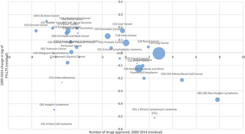1) when N_APP_1948_t is included in the equation. As expected, the coefficient on N_APP_1948_t is negative and highly significant (p-value = 0.0005), indicating that cancer sites with larger increases in the number of drugs ever approved tended to have larger declines in PYLL75. The point estimate of this coefficient implies that, on average, one additional drug approved for a condition reduced PYLL75 by 2.3%. Figure 4 shows the correlation across cancer sites between the 1999–2014 change in the number of drugs ever approved (= the number of drugs approved during 2000–2014) and the 1999–2014 change in the log of PYLL75, controlling for the changes in incidence and mean age at diagnosis.⁷ During the period 1999–2014, PYLL75 due to all types of cancer increased by 4.3%, from 4.23 million to 4.42 million [10]. The population below age 75 increased by 15.4% (from 256.4 million to 299.0 million) during that period, so the premature cancer mortality rate declined by 11.0% (from 1650 to 1477 per 100,000 population). The weighted mean number of drugs approved during 2000–2014 was 6.07, so the estimates of model 2 imply that in the absence of pharmaceutical innovation, PYLL75 due to all types of cancer would have increased by 18.3% (= 4.3% + (.023 * 6.07)), and that the premature cancer mortality rate would have increased by 2.9% (= 18.3% – 15.4%), although the latter increase is probably not statistically significantly different from zero. Also, new cancer drugs reduced PYLL75 at an average annual rate of 0.93% (= (.023 * 6.07)/15) during the period 1999–2014.

Figure 4. Correlation across cancer sites between number of drugs approved during 2000–2014 and 1999–2014 change in log of potential years of life lost before age 75 (PYLL75), controlling for changes in incidence and mean age at diagnosis.

Model 3 in Table 2 corresponds to Equation (A6)(A6) $ln\left(\mathrm{P}\mathrm{Y}\mathrm{L}\mathrm{L}75_{\mathrm{s},\mathrm{t}}\right)={\beta }_{\mathrm{P}\mathrm{R}\mathrm{I}}\mathrm{N}\mathrm{\_}\mathrm{P}\mathrm{R}\mathrm{I}\mathrm{\_}1948\mathrm{\_}{\mathrm{t}}_{\mathrm{s},\mathrm{t}}+{\beta }_{\mathrm{S}\mathrm{T}\mathrm{D}}\mathrm{N}\mathrm{\_}\mathrm{S}\mathrm{T}\mathrm{D}\mathrm{\_}1948\mathrm{\_}{\mathrm{t}}_{\mathrm{s},\mathrm{t}}+\gamma ln(\mathrm{C}\mathrm{A}\mathrm{S}\mathrm{E}{\mathrm{S}}_{\mathrm{s},\mathrm{t}})+\pi \mathrm{A}\mathrm{G}\mathrm{E}\mathrm{\_}\mathrm{D}\mathrm{I}\mathrm{A}{\mathrm{G}}_{\mathrm{s},\mathrm{t}}+{\alpha }_{\mathrm{s}}+{\delta }_{\mathrm{t}}+{\epsilon }_{\mathrm{s},\mathrm{t}}$(A6) , which distinguishes between priority-review and standard-review drugs. The difference between the coefficients on priority-review and standard-review drugs is not statistically significant, so we are unable to reject the null hypothesis that the two types of drugs had equal effects on PYLL75. Model 4 corresponds to Equation (2)(2) $ln\left(\mathrm{S}\mathrm{U}\mathrm{R}\mathrm{V}\mathrm{\_}\mathrm{O}\mathrm{B}{\mathrm{S}}_{\mathrm{s},\mathrm{t}}/\left(1-\mathrm{S}\mathrm{U}\mathrm{R}\mathrm{V}\mathrm{\_}\mathrm{O}\mathrm{B}{\mathrm{S}}_{\mathrm{s},\mathrm{t}}\right)\right)=\beta \mathrm{N}\mathrm{\_}\mathrm{A}\mathrm{P}\mathrm{P}\mathrm{\_}1948\mathrm{\_}{\mathrm{t}}_{\mathrm{s},\mathrm{t}}+\gamma ln\left(\mathrm{C}\mathrm{A}\mathrm{S}\mathrm{E}{\mathrm{S}}_{\mathrm{s},\mathrm{t}}\right)+\pi ln\left(\mathrm{S}\mathrm{U}\mathrm{R}\mathrm{V}\mathrm{\_}\mathrm{E}\mathrm{X}{\mathrm{P}}_{\mathrm{s},\mathrm{t}}/\left(1-\mathrm{S}\mathrm{U}\mathrm{R}\mathrm{V}\mathrm{\_}\mathrm{E}\mathrm{X}{\mathrm{P}}_{\mathrm{s},\mathrm{t}}\right)\right)+{\alpha }_{\mathrm{s}}+{\delta }_{\mathrm{t}}+{\epsilon }_{\mathrm{s},\mathrm{t}}$(2) , which distinguishes between drugs approved more than 4 years before year t and drugs approved 0–4 years before year t. The difference between the coefficients on drugs approved in the two periods is not statistically significant.

In models 5–10 of Table 2, the initial and final years are 1999 and 2010. The estimate of the N_APP_1948_t coefficient in model 6 is larger and more significant than the estimate in model 2 (based on a longer sample period). Models 7 and 8 show that the differences between the coefficients on priority-review and standard-review drugs and between the coefficients on drugs approved more than 4 years before and drugs approved 0–4 years before are again not statistically significant.

Models 9 and 10 include the number of drugs approved 0–4 years after year t. Model 9 does not distinguish between drugs approved more than 4 years before and drugs approved 0–4 years before year t; model 10 does. As expected, the coefficient on the number of drugs approved 0–4 years after year t is not significant in either model. In contrast, in model 10 the coefficient on the number of drugs approved 0–4 years before year t is negative and highly significant.

Table 3 presents estimates of models similar to those presented in Table 2, but in Table 3 the estimates are of models of potential years of life lost before age 65 (PYLL65), rather than age 75. The estimates in Table 3 are qualitatively similar to the estimates in Table 2: the change in log(PYLL65) is strongly inversely related across cancer sites to the number of new drugs approved; the differences between the coefficients on priority-review and standard-review drugs and between the coefficients on drugs approved more than 4 years before and drugs approved 0–4 years before are not statistically significant; and in model 10 the coefficient on the number of drugs approved 0–4 years after year t is not significant, whereas the coefficient on the number of drugs approved 0–4 years before year t is negative and highly significant.

Table 3. Weighted least-squares estimates of models of potential years of life lost before age 65.

	Estimate	Std. Err.	Z	Pr > |Z|	Difference p-value	Estimate	Std. Err.	Z	Pr > |Z|	Difference p-value
	Years 1999, 2014					Years 1999, 2010
	Model 1					Model 5
Δδ	0.1387	0.0281	4.93	<.0001		0.1487	0.0374	3.97	<.0001
	Model 2					Model 6
N_APP_1948_t	−0.0264	0.0055	−4.82	<.0001		−0.0322	0.0058	−5.52	<.0001
Δδ	−0.0631	0.0481	−1.31	0.1894		−0.0510	0.0377	−1.35	0.1756
	Model 3					Model 7
N_PRI_1948_t	−0.0250	0.0088	−2.85	0.0044	0.8031	−0.0307	0.0073	−4.19	<.0001	0.7360
N_STD_1948_t	−0.0288	0.0097	−2.98	0.0029		−0.0369	0.0150	−2.46	0.0141
Δδ	−0.0659	0.0473	−1.39	0.1634		−0.0543	0.0425	−1.28	0.2018
	Model 4					Model 8
N_APP_1948_t-4	−0.0281	0.0052	−5.38	<.0001	0.1280	−0.0327	0.0055	−5.94	<.0001	0.2695
N_APP_t-4_t	−0.0202	0.0069	−2.94	0.0033		−0.0437	0.0080	−5.43	<.0001
Δδ	−0.0749	0.0499	−1.50	0.1333		−0.0120	0.0518	−0.23	0.8170
						Model 9
N_APP_1948_t						−0.0332	0.0059	−5.66	<.0001
N_APP_t_t + 4						0.0056	0.0104	0.53	0.5941
Δδ						−0.0360	0.0402	−0.90	0.3696
						Model 10
N_APP_1948_t-4						−0.0332	0.0060	−5.49	<.0001	0.3209
N_APP_t-4_t						−0.0434	0.0079	−5.51	<.0001
N_APP_t_t + 4						0.0028	0.0111	0.25	0.7989
Δδ						−0.0070	0.0487	−0.14	0.8863

all models include ln(CASES), AGE_DIAG, and cancer-site fixed effects; estimates of these parameters are not shown to conserve space. Δδ denotes the difference between initial and final year fixed effects, e.g. δ₁₉₉₉ – δ₂₀₁₄. Standard errors are clustered within cancer sites. Observations are weighted by mean potential years of life lost before age 65.

3.2. 5-year observed survival rate model estimates

Estimates of models of the observed 5-year survival rate (Equation (2)(2) $ln\left(\mathrm{S}\mathrm{U}\mathrm{R}\mathrm{V}\mathrm{\_}\mathrm{O}\mathrm{B}{\mathrm{S}}_{\mathrm{s},\mathrm{t}}/\left(1-\mathrm{S}\mathrm{U}\mathrm{R}\mathrm{V}\mathrm{\_}\mathrm{O}\mathrm{B}{\mathrm{S}}_{\mathrm{s},\mathrm{t}}\right)\right)=\beta \mathrm{N}\mathrm{\_}\mathrm{A}\mathrm{P}\mathrm{P}\mathrm{\_}1948\mathrm{\_}{\mathrm{t}}_{\mathrm{s},\mathrm{t}}+\gamma ln\left(\mathrm{C}\mathrm{A}\mathrm{S}\mathrm{E}{\mathrm{S}}_{\mathrm{s},\mathrm{t}}\right)+\pi ln\left(\mathrm{S}\mathrm{U}\mathrm{R}\mathrm{V}\mathrm{\_}\mathrm{E}\mathrm{X}{\mathrm{P}}_{\mathrm{s},\mathrm{t}}/\left(1-\mathrm{S}\mathrm{U}\mathrm{R}\mathrm{V}\mathrm{\_}\mathrm{E}\mathrm{X}{\mathrm{P}}_{\mathrm{s},\mathrm{t}}\right)\right)+{\alpha }_{\mathrm{s}}+{\delta }_{\mathrm{t}}+{\epsilon }_{\mathrm{s},\mathrm{t}}$(2) ) are presented in Table 4. These estimates are based on data for the years 2000 and 2008 from all 18 SEER registries, 5 of which began providing data in 2000. Since the survival rate is ‘forward-looking,’ the 2008 data are the most recent available data. The number of patients diagnosed in all registries increased from 263,848 in 2000 to 287,954 in 2008. Between 2000 and 2008, the observed survival rate for all cancers combined increased from 56.1% to 60.3%, the expected survival rate increased from 86.5% to 88.6%, and the relative survival rate increased from 64.9% to 68.0%. Observations are weighted by number of patients diagnosed. All models in Table 4 include ln(CASES), ln(SURV_EXP/(1 – SURV_EXP)), and cancer-site fixed effects. As expected, the coefficients on ln(CASES) and ln(SURV_EXP/(1 – SURV_EXP)) are both positive and highly significant in all models: observed survival increased more for cancers that had larger increases in the number of people diagnosed and larger increases in expected survival (e.g. due to earlier diagnosis).

Table 4. Weighted least-squares estimates of models of the observed 5-year survival rate (Equation (2)(2) $ln\left(\mathrm{S}\mathrm{U}\mathrm{R}\mathrm{V}\mathrm{\_}\mathrm{O}\mathrm{B}{\mathrm{S}}_{\mathrm{s},\mathrm{t}}/\left(1-\mathrm{S}\mathrm{U}\mathrm{R}\mathrm{V}\mathrm{\_}\mathrm{O}\mathrm{B}{\mathrm{S}}_{\mathrm{s},\mathrm{t}}\right)\right)=\beta \mathrm{N}\mathrm{\_}\mathrm{A}\mathrm{P}\mathrm{P}\mathrm{\_}1948\mathrm{\_}{\mathrm{t}}_{\mathrm{s},\mathrm{t}}+\gamma ln\left(\mathrm{C}\mathrm{A}\mathrm{S}\mathrm{E}{\mathrm{S}}_{\mathrm{s},\mathrm{t}}\right)+\pi ln\left(\mathrm{S}\mathrm{U}\mathrm{R}\mathrm{V}\mathrm{\_}\mathrm{E}\mathrm{X}{\mathrm{P}}_{\mathrm{s},\mathrm{t}}/\left(1-\mathrm{S}\mathrm{U}\mathrm{R}\mathrm{V}\mathrm{\_}\mathrm{E}\mathrm{X}{\mathrm{P}}_{\mathrm{s},\mathrm{t}}\right)\right)+{\alpha }_{\mathrm{s}}+{\delta }_{\mathrm{t}}+{\epsilon }_{\mathrm{s},\mathrm{t}}$(2) ).

Parameter	Estimate	Std. Err.	Z	Pr > |Z|	Difference p-value
	Years 2000, 2008
	Model 1
δ2000 – δ2008	−0.0971	0.0557	−1.74	0.0810
	Model 2
N_APP_1948_t	0.0240	0.0087	2.77	0.0056
δ2000 – δ2008	−0.0158	0.0528	−0.30	0.7654
	Model 3
N_PRI_1948_t	0.0471	0.0098	4.82	<.0001	0.0005
N_STD_1948_t	−0.0389	0.0200	−1.94	0.0519
δ2000 – δ2008	−0.0294	0.0491	−0.60	0.5501
	Model 4
N_APP_1948_t-4	0.0353	0.0093	3.78	0.0002	0.0003
N_APP_t-4_t	0.0212	0.0091	2.33	0.0200
δ2000 – δ2008	−0.0443	0.0569	−0.78	0.4362
	Model 5
N_APP_1948_t-8	0.0257	0.0089	2.88	0.0040	0.4546
N_APP_t-8_t	0.0214	0.0100	2.14	0.0327
δ2000 – δ2008	−0.0301	0.0594	−0.51	0.6121

all models include ln(CASES), ln(SURV_EXP/(1 – SURV_EXP)), and cancer-site fixed effects; estimates of these parameters are not shown to conserve space. Standard errors are clustered within cancer sites. Observations are weighted by number of patients diagnosed.

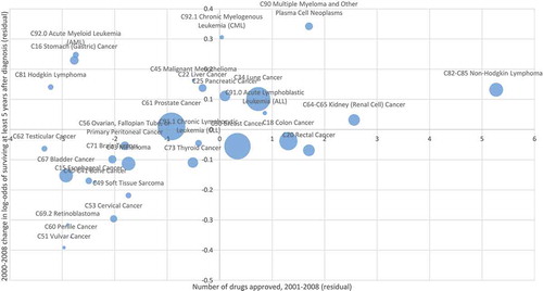
Model 1 of Table 4 indicates that, holding constant the number of people diagnosed and the expected survival rate, between 2000 and 2008 the odds of surviving for at least 5 years after diagnosis increased 10.2% (= exp(δ₂₀₀₈ – δ₂₀₀₀) – 1), although the increase is only marginally significant (p-value = .0810). Model 2 includes the number of drugs approved until year t (N_APP_1948_t). The coefficient on this variable is positive and highly significant (p-value = .0056). The point estimate indicates that one additional drug approval increases the odds of surviving 5 years by 2.4%. Figure 5 shows the correlation across cancer sites between the number of drugs approved during 2001–2008 and the 2000–2008 change in the log-odds of surviving at least 5 years after diagnosis, controlling for changes in incidence and the expected survival rate.

Figure 5. Correlation across cancer sites between number of drugs approved during 2001–008 and 2000–2008 change in log-odds of surviving at least 5 years after diagnosis, controlling for changes in incidence and expected survival rate.

Model 3 distinguishes between priority-review and standard-review drugs. The coefficient on the former is positive and highly significant, whereas the coefficient on the latter is negative and marginally significant; the difference between the coefficients is highly significant. Model 4 distinguishes between drugs approved more than 4 years before and drugs approved 0–4 years before. The coefficients on both variables are positive and significant, but the coefficient on more recent drug approvals is significantly larger. Model 5 distinguishes between drugs approved more than 8 years before and drugs approved 0–8 years before. Once again, the coefficients on both variables are positive and significant, but in this case the difference between the coefficients is not statistically significant.

3.3. Hospital days model estimates

Now we will present estimates of several versions of the model of cancer patient hospital days (Equation (3)(3) $ln\left(\mathrm{H}\mathrm{O}\mathrm{S}\mathrm{P}\mathrm{\_}\mathrm{D}\mathrm{A}\mathrm{Y}{\mathrm{S}}_{\mathrm{s},\mathrm{t}}\right)=\beta \mathrm{N}\mathrm{\_}\mathrm{A}\mathrm{P}\mathrm{P}\mathrm{\_}1948\mathrm{\_}{\mathrm{t}}_{\mathrm{s},\mathrm{t}}+\gamma ln\left(\mathrm{C}\mathrm{A}\mathrm{S}\mathrm{E}{\mathrm{S}}_{\mathrm{s},\mathrm{t}}\right)+\pi \mathrm{A}\mathrm{G}\mathrm{E}\mathrm{\_}\mathrm{D}\mathrm{I}\mathrm{A}{\mathrm{G}}_{\mathrm{s},\mathrm{t}}+{\alpha }_{\mathrm{s}}+{\delta }_{\mathrm{t}}+{\epsilon }_{\mathrm{s},\mathrm{t}}$(3) ). The initial and final years of this analysis are 1997 and 2013, respectively. During that period, the number of cancer patient hospital days declined 22.1%, from 11.7 million to 9.1 million, despite the fact that the average annual number of patients diagnosed with cancer in SEER 9 registries increased by 29%. Model 1 of Table 5 indicates that, holding constant the number of patients diagnosed and their mean age, the number of cancer patient hospital days declined 32% (= 1 – exp(δ₂₀₁₃ – δ₁₉₉₇)). Model 2 includes the number of drugs approved until year t. The coefficient on this variable is negative, as expected, but only marginally significant (p-value = 0.077). Model 3 distinguishes between priority-review and standard-review drugs; the difference between these coefficients is not significant. Model 4 distinguishes between drugs approved more than 4 years before and drugs approved 0–4 years before. Only the coefficient on the number of drugs approved more than 4 years before is statistically significant. Model 5 distinguishes between drugs approved more than 8 years before and drugs approved 0–8 years before. Only the coefficient on the number of drugs approved more than 8 years before is statistically significant. The estimate of (δ₁₉₉₇ – δ₂₀₁₃) in model 5 implies that, in the absence of (lagged) pharmaceutical innovation (i.e. holding constant the number of drugs approved 8 years before, as well as the number of patients diagnosed and their mean age), the number of hospital days would have declined by 19.1%. Thus we estimate that lagged pharmaceutical innovation resulted in a 13.3% decline in the number of cancer patient hospital days during the period 1997–2013. Also, new cancer drugs reduced the number of cancer patient hospital days at an average annual rate of 0.83% (= 13.3%/16) during the period 1997–2013.

Table 5. Weighted least-squares estimates of models of the number of hospital days (Equation (3)(3) $ln\left(\mathrm{H}\mathrm{O}\mathrm{S}\mathrm{P}\mathrm{\_}\mathrm{D}\mathrm{A}\mathrm{Y}{\mathrm{S}}_{\mathrm{s},\mathrm{t}}\right)=\beta \mathrm{N}\mathrm{\_}\mathrm{A}\mathrm{P}\mathrm{P}\mathrm{\_}1948\mathrm{\_}{\mathrm{t}}_{\mathrm{s},\mathrm{t}}+\gamma ln\left(\mathrm{C}\mathrm{A}\mathrm{S}\mathrm{E}{\mathrm{S}}_{\mathrm{s},\mathrm{t}}\right)+\pi \mathrm{A}\mathrm{G}\mathrm{E}\mathrm{\_}\mathrm{D}\mathrm{I}\mathrm{A}{\mathrm{G}}_{\mathrm{s},\mathrm{t}}+{\alpha }_{\mathrm{s}}+{\delta }_{\mathrm{t}}+{\epsilon }_{\mathrm{s},\mathrm{t}}$(3) ).

Parameter	Estimate	Std. Err.	Z	Pr > |Z|	Difference p-value
	Years 1997, 2013
	Model 1
δ1997 – δ2013	0.3913	0.0741	5.28	<.0001
	Model 2
N_APP_1948_t	−0.0195	0.0110	−1.77	0.0769
δ1997 – δ2013	0.2789	0.0801	3.48	0.0005
	Model 3
N_PRI_1948_t	−0.0351	0.03	−1.17	0.2439	0.5592
N_STD_1948_t	0.0037	0.04	0.09	0.9268
δ1997 – δ2013	0.2838	0.078	3.64	0.0003
	Model 4
N_APP_1948_t-4	−0.0224	0.0101	−2.22	0.0265	0.0854
N_APP_t-4_t	0.0211	0.0243	0.87	0.3848
δ1997 – δ2013	0.2293	0.0859	2.67	0.0076
	Model 5
N_APP_1948_t-8	−0.0291	0.0124	−2.34	0.0192	0.0610
N_APP_t-8_t	−0.0028	0.0125	−0.23	0.8213
δ1997 – δ2013	0.2115	0.0947	2.23	0.0256

all models include ln(CASES), AGE_DIAG, and cancer-site fixed effects; estimates of these parameters are not shown to conserve space. Standard errors are clustered within cancer sites. Observations are weighted by mean number of hospital days.

4. Cost-effectiveness estimation

Now we will use some of the estimates described in the previous section along with some other data to produce a baseline estimate of the average cost-effectiveness in 2014 of cancer drugs approved by the FDA during the period 2000–2014. The cost-effectiveness measure we will use is cost per life-year gained: the ratio of the cost in 2014 of drugs approved during the period 2000–2014 (net of rebates and two types of ‘cost offsets’) to the number of life-years gained in 2014 attributable to those drugs.⁸

Calculation of cost-effectiveness is described in Table A4. As shown in line 1, according to the IMS Institute for Healthcare Informatics, total U.S. expenditure (before rebates) on cancer drugs in 2014 was $32.3 billion [11].⁹ Unpublished IMS MIDAS data indicate that 67.7% of 2014 cancer drug expenditure was on drugs approved after 1999 (line 2), so we estimate that 2014 expenditure (before rebates) on cancer drugs approved after 1999 was $21.9 billion (line 3). However, the net social cost of these drugs is considerably lower than that, for three reasons: rebates, reduced expenditure on old drugs, and reduced hospital expenditure. We address these in turn.

Rebates. Drug rebates are believed to be pervasive, but are notoriously difficult to measure. Herper provided estimates of the effective rebates on 10 top-selling drugs (but not specifically cancer drugs) by comparing gross (pre-rebate) sales figures (reported to IMS Health) to net (post-rebate) sales figures (in company financial statements) [12]. Based on that methodology, he estimated that the weighted average rebate rate was 25%.¹⁰ We therefore assume that rebates on post-1999 cancer drugs amounted to $5.5 billion (line 4 of Table A4). Therefore, net sales of these drugs was $16.4 billion.

Reduced expenditure on old drugs. Lichtenberg showed that, in general, ‘about one-fourth of the … increase in new drug cost [is] offset by a reduction in old drug cost [13].’ Once again, this estimate was based on data on (outpatient) drugs in general, not specifically on cancer drugs.¹¹ But if it also applies to cancer drugs, then the $16.4 billion net expenditure on new cancer drugs would reduce old cancer drug expenditure by $4.1 billion (line 5).

Reduced hospital expenditure. The estimate of Δδ in model 1 of Table 5 implies that, holding constant the number of patients diagnosed and their mean age, HOSP_DAYS declined by 32.4% (= exp(-Δδ) – 1) between 1997 and 2013. In 1997, HOSP_DAYS was 11.7 million, so this represents a HOSP_DAYS reduction of 3.78 million (= 32.4% * 11.7 million). The estimate of Δδ in model 5 of Table 5 implies that, in the absence of pharmaceutical innovation, HOSP_DAYS would have declined by 19.1%, or 2.22 million (= 19.1% * 11.7 million). Hence cancer drugs approved between 1989 and 2005 are estimated to have reduced HOSP_DAYS in 2013 by 1.55 million. In 2013, average cost per cancer patient hospital day was $3076.¹² Assuming that hospital costs are proportional to hospital days,¹³ this implies that cancer drugs approved between 1989 and 2005 reduced hospital costs in 2013 by $4.77 billion (= $3076 * 1.55 million). This is shown in line 6 of Table A4.

As shown in line 7, the estimated net social cost of post-1999 cancer drugs in 2014, after accounting for rebates and reduced expenditure on old drugs and hospital care, is $7.5 billion. This represents expenditure on all patients. We want to estimate expenditure on patients below the age of 75, because the denominator of the cost-effectiveness ratio we will use is life-years gained before age 75. SEER data indicate that about 75% of cancer patients are diagnosed before the age of 75. As shown in line 8, we will assume that 75% of the net cost of post-1999 cancer drugs in 2014 was on patients below the age of 75,¹⁴ so net expenditure on these patients was $5.6 billion.

The estimates in Table 2 can be used to calculate the number of life-years gained before age 75 in 2014 from cancer drugs approved during 2000–2014, controlling for changes in incidence and mean age at diagnosis. The estimate of Δδ in model 1 of Table 2 implies that, holding constant the number of patients diagnosed and their mean age, PYLL75 declined by 7.6% (= exp(-Δδ) – 1) between 1999 and 2014. In 1999, PYLL75 was 4.229 million, so this represents a PYLL75 reduction of 323,186 (= 7.6% * 4.229 million). The estimate of Δδ in model 2 of Table 2 implies that, in the absence of pharmaceutical innovation, PYLL75 would have increased by 9.4%, or 395,947 (= 9.4% * 4.229 million). Hence, as shown in line 9 of Table A4, cancer drugs approved during 2000–2014 are estimated to have reduced PYLL75 in 2014 by 719,133 (= 323,186 + 395,947).

Our baseline estimate of the cost per life-year gained in 2014 from cancer drugs approved during 2000–2014 is $7853 (line 10). Performing sensitivity analyses by modifying the estimates or assumptions described in Table A4 is straightforward. For example, if we completely ignore the estimated reductions in old drug and hospital expenditure, the estimated cost per life-year gained is $17,104.

Even the higher estimate would imply that, overall, cancer drug innovation has been highly cost-effective, by the standards of the World Health Organization and other authorities [14]. The World Health Organization considers interventions whose cost per quality-adjusted life-year (QALY) gained is less than 3 times per capita GDP to be cost-effective, and those whose cost per QALY gained is less than per capita GDP to be highly cost-effective [15]; US per capita GDP in 2014 was $54,697.

Our baseline estimate of the cost per life-year before age 75 gained in the U.S. in 2014 from cancer drugs approved during 2000–2014 is roughly consistent with a previous study’s estimate of the cost per life-year before age 75 gained in 36 countries in 2015 from drugs launched during 2006–2010: $2,276 [16]. An analysis of unpublished data from IMS Health indicates that the average price of cancer drugs outside the U.S. is about 55% of the U.S. price.¹⁵

However, our estimate of average cost-effectiveness based on population-based observational research is considerably lower than almost all estimates derived from clinical trials of the cost-effectiveness of individual drugs reported by Cressman et al [17]. (Since many new drugs are introduced for small groups of patients, it isn’t possible to determine average cost-effectiveness from Cressman et al’s data.) A number of factors may contribute to this discrepancy. (1) Many of the estimates compiled by Cressman et al are of cost per progression-free life-year gained (PFLYG), whereas we estimate cost per life-year gained. (2) Estimates of costs of individual drugs may be based on list prices, and may not account for rebates. (3) RCT-based estimates of PFLYG generally don’t account for ‘cost offsets’; we estimated that lagged pharmaceutical innovation resulted in a 13.3% decline in the number of cancer patient hospital days during the period 1997–2013.

5. Conclusion

Cancer drug innovation has been accelerating: more than 8 times as many new cancer drugs were approved during 2005–2015 as were approved during 1975–1985 (66 vs. 8). The average annual 2010–2014 growth rate of U.S. cancer drug expenditure was 7.6%–more than 3.6 times the average annual growth rate of nominal U.S. GDP. This has contributed to a lively debate about the value and cost-effectiveness of new cancer drugs. In this population-based observational research study, we assessed the average cost-effectiveness in the U.S. in 2014 of new cancer drugs approved by the FDA during 2000–2014, by investigating whether there were larger declines in premature mortality and hospitalization, and larger increases in survival, from the cancers that had larger increases in the number of drugs ever approved, controlling for the change in cancer incidence and mean age at time of diagnosis.

Cancer drugs approved during 2000–2014 are estimated to have reduced the number of potential years of life lost before age 75 in 2014 by 719,133. Cancer drugs approved during 1989–2005 are estimated to have reduced hospital cost in 2013 by $4.8 billion. Our baseline estimate of the cost per life-year gained in 2014 from cancer drugs approved during 2000–2014 is $7853.

6. Expert opinion

Some authors have argued that most new drugs in general, and most new cancer drugs in particular, have not provided real advances over existing drugs. Wieseler, McGauran, and Kaiser said that the proportion of ‘true innovation’ is less than 15% [18]. Davis et al said that most cancer drugs approved by the EMA between 2009 and 2013 had been approved with no evidence of clinically meaningful benefit on patient relevant outcomes (survival and quality of life) [19]. A systematic review by Pease et al of new drugs for over 100 indications approved by the US Food and Drug Administration on the basis of limited evidence found that superior efficacy on clinical outcomes was confirmed in less than 10% of cases [20]. For cancer drugs, according to Gyawali, Hey, and Kesselheim, superior efficacy on clinical outcomes was confirmed in less than 20% of cases [21]. However, an aphorism ‘beloved of forensic scientists’ and cited by Alderson is that ‘absence of evidence is not evidence of absence [22,23].’

If most new cancer drugs have not provided real advances over existing drugs, there should be little or no correlation across cancer sites between the number of new drugs launched and changes in premature mortality, survival, and hospitalization rates, controlling for changes in incidence, mean age at diagnosis, and expected survival. But in this article, we have shown that there are highly significant correlations across cancer sites between the number of new drugs launched in the U.S. and changes in outcomes of American cancer patients (Figures 4 and 5). Moreover, the estimates indicated that, overall, the drugs have been highly cost-effective as well as clinically effective.

Several previous studies, based on data from many countries, have provided evidence consistent with that finding. One study showed that there is also a highly significant inverse correlation across 36 countries between relative mortality from 19 types of cancer in 2015 and the relative number of drugs previously launched in that country to treat that type of cancer, controlling for relative incidence [16]. Another study, of all types of diseases, showed that the rate of decline of mortality from disease d in country c during 2000–2013 was significantly inversely related to the change in the number of drugs to treat that disease previously launched in that country, controlling for the average rates of mortality decline from each disease and in each country [24]. A third study showed that the larger the relative number of drugs for a disease that were launched during 1982–2015 in a country, the lower the relative disability in 2015 of patients with that disease in that country, controlling for the average level of disability in that country and from that disease, and the number of patients with the disease and their mean age [25].

The authors who have claimed that most new cancer drugs have not provided real advances over existing drugs have relied entirely on systematic reviews of data from randomized clinical trials. Frieden argued that ‘although randomized, controlled trials have long been presumed to be the ideal source for data on the effects of treatment, other methods of obtaining evidence for decisive action are receiving increased interest, prompting new approaches to leverage the strengths and overcome the limitations of different data sources’; moreover, ‘observational studies, including assessments of results from the implementation of new programs and policies, remain the foremost [other method of obtaining evidence] [26].’¹⁶ Booth and Tannock observed that ‘although randomization minimizes the risk of bias by confounding, there are other biases inherent to RCTs that limit their applicability to the care of patients in routine practice. In particular, patients, providers, and concurrent care in the general population are different from those in clinical trials, and the generalizability (or external validity) of RCTs may be limited. Although population-based observational research does not enjoy the same level of internal validity at RCTs, well-designed observational studies can offer superior external validity and provide a unique opportunity to evaluate the uptake of new treatments and their outcomes in routine practice [27].’ Also, Deaton and Cartwright said that ‘the lay public, and sometimes researchers, put too much trust in RCTs over other methods of investigation,’ and that ‘any special status for RCTs is unwarranted’; ‘an observational study with credible corrections and a more relevant and much larger study sample – today often the complete population of interest through administrative records, where blinding and selection issues are absent – may provide a better estimate [28].’

In general, new cancer drugs may be far more cost-effective than data based on clinical trials appear to suggest: our estimate of average cost-effectiveness based on population-based observational research is considerably lower than almost all estimates derived from clinical trials of individual drugs. Policymakers should be aware of this when they assess the cost-effectiveness of new cancer drugs. Authors of previous studies have argued that well-designed observational studies can offer superior external validity and provide a unique opportunity to evaluate the uptake of new treatments and their outcomes in routine practice. Reconciliation of the findings of two main research approaches – RCTs and population-based observational research – is a task for future research.

Article Highlights

• Cancer sites with larger increases in the number of drugs ever approved tended to have larger declines in the number of potential years of life lost before ages 75 and 65.

• On average, one additional drug approved for a cancer site reduced the number of potential years of life lost before age 75 by 2.3%.

• New cancer drugs reduced the number of potential years of life lost before age 75 at an average annual rate of 0.93% during the period 1999–2014.

• Cancer drugs approved during 2000–2014 are estimated to have reduced the number of potential years of life lost before age 75 in 2014 by 719,133

• Premature mortality in year t is strongly inversely related to the number of drugs approved in years t-3 to t (and earlier years), but unrelated to the number of drugs approved in years t+1 to t+4.

• One additional drug approval increases the odds of surviving at least 5 years after diagnosis by 2.4%.

• New cancer drugs reduced the number of cancer patient hospital days at an average annual rate of 0.83% during the period 1997–2013.

• Cancer drugs approved between 1989 and 2005 are estimated to have reduced the number of hospital days in 2013 by 1.55 million, and hospital cost in 2013 by $4.8 billion.

• Our baseline estimate of the cost per life-year gained in 2014 from cancer drugs approved during 2000–2014 is $7853. If we completely ignore the estimated reductions in old drug and hospital expenditure, the estimated cost per life-year gained is $17,104. Even the higher estimate would imply that, overall, cancer drug innovation has been highly cost-effective, by the standards of the World Health Organization and other authorities.

Declaration of interest

The author has no relevant affiliations or financial involvement with any organization or entity with a financial interest in or financial conflict with the subject matter or materials discussed in the manuscript. This includes employment, consultancies, honoraria, stock ownership or options, expert testimony, grants or patents received or pending, or royalties.

Reviewer Disclosures

Peer reviewers on this manuscript have no relevant financial or other relationships to disclose.

Additional information

Funding

Financial support for this research was provided by Incyte Corporation.

Notes

1. Burnet et al argued that ‘years of life lost (YLL) from cancer is an important measure of population burden – and should be considered when allocating research funds [42].’

2. Many drugs are used to treat more than one type of cancer.

3. New drug approvals can improve outcomes for 2 reasons. First, the quality of newer products may be higher than the quality of older products, as in ‘quality ladder’ models [31]. Second, ‘one of the principal means, if not the principal means, through which countries benefit from international trade is by the expansion of varieties’ [43].

4. A similar model of potential years of life lost before age 65 will also be estimated.

5. 1949 was the first year in which a cancer drug included in the National Cancer Institute’s lists of cancer drugs was approved by the FDA [1].

6. Some studies have found no mortality benefit from more intensive screening. For example, data from the Prostate, Lung, Colorectal and Ovarian randomized screening trial showed that, after 13 years of follow up, men who underwent annual prostate cancer screening with prostate-specific antigen testing and digital rectal examination had a 12 percent higher incidence of prostate cancer than men in the control group but the same rate of death from the disease. No evidence of a mortality benefit was seen in subgroups defined by age, the presence of other illnesses, or pre-trial PSA testing [44].

7. This figure shows the correlation between the residual from the regression of Δln(PYLL75_s) on Δln(CASES_s) and ΔAGE_DIAG_s and the residual from the regression of ΔN_APP_1948_t_s on Δln(CASES_s) and ΔAGE_DIAG_s (see eq. (4)).

8. We would prefer to measure cost per quality-adjusted life-year (QALY) gained, but systematic data on the average quality of life of cancer patients, by cancer site and year, are not available. The cost per QALY could be either greater than or less than the cost per life-year, because the number of QALYs gained could be either less than or greater than the number of life-years gained. Although patients’ quality of life in the marginal years (the additional life-years gained) is undoubtedly less than perfect, pharmaceutical innovation may also increase quality of life in the infra-marginal years.

9. This figure is 11% higher than the estimate given in Table A1. To be conservative, we will use the higher figure.

10. Herper quotes a principal at a pharmaceutical marketing consultancy, who said that ‘the size of the rebate average[s] about 30% of a medicine’s sales [12].’

11. To calculate that estimate, Lichtenberg used data from the Medical Expenditure Panel Survey on average utilization of new and old drugs by medical condition (disease) and year [13]. Unfortunately, data on average utilization of new and old drugs by cancer site and year are not available. As discussed above, although data are available on the total use of new cancer drugs, many cancer drugs are used for several types of cancer, and data on the use of cancer drugs for each type of cancer are not available.

12. The aggregate cost of cancer patient hospitalization was $27.9 billion, and the aggregate number of hospital days was 9.1 million [9]. Costs tend to reflect the actual costs of production, while charges represent what the hospital billed for the case. Total charges were converted to costs using cost-to-charge ratios based on hospital accounting reports from the Centers for Medicare and Medicaid Services (CMS). Hospital charges is the amount the hospital charged for the entire hospital stay. It does not include professional (MD) fees. Charges are not necessarily how much was reimbursed.

13. The assumption that a reduction in hospital costs is proportional to a reduction in hospital days might not hold. Typically the last days in hospital are cheaper.

14. The true fraction of expenditure could be higher or lower. Treatments given to younger patients could be more expensive; on the other hand, people diagnosed before age 75 may continue to receive treatments after age 75.

15. This relative price was calculated by estimating the following model by weighted least squares, weighting by the number of standard units, using 2014 data on 107 molecules: ln(P_mr) = δ_r + α_m + ε_mr, where P_mr = manufacturer revenue per standard unit of molecule m in region r (r = USA, ROW (rest of the world)).

Table

Parameter	Estimate	Std. Err.	t Value	Pr > |t|
δROW – δUSA	−0.591	0.093	6.37	<.0001

16. The FDA uses real world data and real world evidence (RWE) to monitor postmarket safety and adverse events and to make regulatory decisions. The 21st Century Cures Act, passed in 2016, places additional focus on the use of these types of data to support regulatory decision making, including approval of new indications for approved drugs. Congress defined RWE as data regarding the usage, or the potential benefits or risks, of a drug derived from sources other than traditional clinical trials [45].

17. Moreover, the medical substances and devices sector was the most R&D-intensive major industrial sector: almost twice as R&D-intensive as the next-highest sector (information and electronics), and three times as R&D-intensive as the average for all major sectors [46]. R&D intensity is the ratio of R&D to sales.

18. Dorsey ER (2010). Financial Anatomy of Biomedical Research, 2003-2008.  Journal of the American Medical Association 303(2): 137-143, January 13.

19. 63% of the cancer drugs approved during 1949–2015 were given priority review designation. Since the FDA’s classification of a drug (priority vs. standard review) occurs at the beginning of the review process, it may be subject to considerable uncertainty; the fact that some drugs are withdrawn after marketing indicates that even the safety of a drug may not be well understood at the time of approval.

20. First-in-class drugs are much more likely to receive priority-review status than follow-on drugs, so distinguishing between priority-review and standard-review drugs is similar to distinguishing between first-in-class and follow-on drugs.

21. Since the dependent variable of Equation (A1)(A1) $ln\left(\mathrm{P}\mathrm{Y}\mathrm{L}\mathrm{L}{75}_{\mathrm{s},1999}\right)=\beta \mathrm{N}\mathrm{\_}\mathrm{A}\mathrm{P}\mathrm{P}\mathrm{\_}1948\mathrm{\_}{\mathrm{t}}_{\mathrm{s},1999}+\gamma ln\left(\mathrm{C}\mathrm{A}\mathrm{S}\mathrm{E}{\mathrm{S}}_{\mathrm{s},1999}\right)+\pi \mathrm{A}\mathrm{G}\mathrm{E}\mathrm{\_}\mathrm{D}\mathrm{I}\mathrm{A}{\mathrm{G}}_{\mathrm{s},1999}+{\alpha }_{\mathrm{s}}+{\delta }_{1999}+{\epsilon }_{\mathrm{s},1999}$(A1) is logarithmic, observations for which N_SU_mn = 0 had to be excluded.

Appendices

Appendix 1.

Specification and estimation of premature cancer mortality model Equation (1)(1) $ln\left(\mathrm{P}\mathrm{Y}\mathrm{L}\mathrm{L}{75}_{\mathrm{s},\mathrm{t}}\right)=\beta \mathrm{N}\mathrm{\_}\mathrm{A}\mathrm{P}\mathrm{P}\mathrm{\_}1948\mathrm{\_}{\mathrm{t}}_{\mathrm{s},\mathrm{t}}+\gamma ln\left(\mathrm{C}\mathrm{A}\mathrm{S}\mathrm{E}{\mathrm{S}}_{\mathrm{s},\mathrm{t}}\right)+\pi \mathrm{A}\mathrm{G}\mathrm{E}\mathrm{\_}\mathrm{D}\mathrm{I}\mathrm{A}{\mathrm{G}}_{\mathrm{s},\mathrm{t}}+{\alpha }_s+{\delta }_t+{\epsilon }_{\mathrm{s},\mathrm{t}}$(1)

Background. Longevity increase (or declining mortality rates) is a very important part of economic growth, broadly defined. Nordhaus argued that ‘improvements in health status have been a major contributor to economic welfare over the twentieth century. To a first approximation, the economic value of increases in longevity in the last hundred years is about as large as the value of measured growth in non-health goods and services [29].’ The United Nations’ Human Development Index (HDI) is a composite statistic of life expectancy, education, and income per capita indicators, which are used to rank countries into four tiers of human development [30].

Building on a large collection of previous research by Romer, Grossman and Helpman, Aghion and Howitt, and others, Jones presented a model in which ‘long-run growth is driven by the discovery of new ideas throughout the world [31–34].’ He postulated an aggregate production function in which total output depends on the total stock of ideas available to this economy as well as on physical and human capital.

In general, measuring the number of ideas is challenging. One potential measure is the number of patents, but Patterson noted that only 1% of patent applications made by Bell Labs ‘generated [commercial] value [35].’ Fortunately, due to FDA regulation, measuring pharmaceutical ‘ideas’ is considerably easier than measuring ideas in general.¹⁷ The measure of pharmaceutical ideas we will use is the number of new molecular entities approved by the FDA. Since we have precise information about when those ideas reached the market and the diseases to which they apply, we can assess the impact of those ideas on longevity and hospitalization in a difference-in-differences framework. We therefore believe that Nordhaus may have been unduly skeptical when he wrote that ‘we cannot at this stage attribute the growth in health income to particular investments or expenditures’ and that ‘apply[ing] the techniques of growth accounting to health improvements … is especially challenging [29].’

Estimation details. The standard errors of Equation (1)(1) $ln\left(\mathrm{P}\mathrm{Y}\mathrm{L}\mathrm{L}{75}_{\mathrm{s},\mathrm{t}}\right)=\beta \mathrm{N}\mathrm{\_}\mathrm{A}\mathrm{P}\mathrm{P}\mathrm{\_}1948\mathrm{\_}{\mathrm{t}}_{\mathrm{s},\mathrm{t}}+\gamma ln\left(\mathrm{C}\mathrm{A}\mathrm{S}\mathrm{E}{\mathrm{S}}_{\mathrm{s},\mathrm{t}}\right)+\pi \mathrm{A}\mathrm{G}\mathrm{E}\mathrm{\_}\mathrm{D}\mathrm{I}\mathrm{A}{\mathrm{G}}_{\mathrm{s},\mathrm{t}}+{\alpha }_s+{\delta }_t+{\epsilon }_{\mathrm{s},\mathrm{t}}$(1) will be clustered within cancer sites. The data exhibit heteroscedasticity. For example, cancer sites with larger mean premature mortality during 1999–2014 had smaller (positive and negative) annual percentage fluctuations in PYLL75_st. Equation (1)(1) $ln\left(\mathrm{P}\mathrm{Y}\mathrm{L}\mathrm{L}{75}_{\mathrm{s},\mathrm{t}}\right)=\beta \mathrm{N}\mathrm{\_}\mathrm{A}\mathrm{P}\mathrm{P}\mathrm{\_}1948\mathrm{\_}{\mathrm{t}}_{\mathrm{s},\mathrm{t}}+\gamma ln\left(\mathrm{C}\mathrm{A}\mathrm{S}\mathrm{E}{\mathrm{S}}_{\mathrm{s},\mathrm{t}}\right)+\pi \mathrm{A}\mathrm{G}\mathrm{E}\mathrm{\_}\mathrm{D}\mathrm{I}\mathrm{A}{\mathrm{G}}_{\mathrm{s},\mathrm{t}}+{\alpha }_s+{\delta }_t+{\epsilon }_{\mathrm{s},\mathrm{t}}$(1) will therefore be estimated by weighted least-squares, weighting by Σ_t PYLL75_st. This specification imposes the property of diminishing marginal productivity of drug approvals.

Other potential determinants. Due to data limitations, Equation (1)(1) $ln\left(\mathrm{P}\mathrm{Y}\mathrm{L}\mathrm{L}{75}_{\mathrm{s},\mathrm{t}}\right)=\beta \mathrm{N}\mathrm{\_}\mathrm{A}\mathrm{P}\mathrm{P}\mathrm{\_}1948\mathrm{\_}{\mathrm{t}}_{\mathrm{s},\mathrm{t}}+\gamma ln\left(\mathrm{C}\mathrm{A}\mathrm{S}\mathrm{E}{\mathrm{S}}_{\mathrm{s},\mathrm{t}}\right)+\pi \mathrm{A}\mathrm{G}\mathrm{E}\mathrm{\_}\mathrm{D}\mathrm{I}\mathrm{A}{\mathrm{G}}_{\mathrm{s},\mathrm{t}}+{\alpha }_s+{\delta }_t+{\epsilon }_{\mathrm{s},\mathrm{t}}$(1) does not include other disease-specific, time-varying, explanatory variables. But both a patient-level U.S. study and a longitudinal country-level study have shown that controlling for numerous other potential determinants of longevity does not reduce, and may even increase, the estimated effect of pharmaceutical innovation. The study based on patient-level data found that controlling for race, education, family income, insurance coverage, Census region, BMI, smoking, the mean year the person started taking his or her medications, and over 100 medical conditions had virtually no effect on the estimate of the effect of pharmaceutical innovation (the change in drug vintage) on life expectancy [36]. The study based on longitudinal country-level data found that controlling for ten other potential determinants of longevity change (real per capita income, the unemployment rate, mean years of schooling, the urbanization rate, real per capita health expenditure (public and private), the DPT immunization rate among children ages 12–23 months, HIV prevalence and tuberculosis incidence) increased the coefficient on pharmaceutical innovation by about 32% [37].

Failure to control for non-pharmaceutical medical innovation (e.g. innovation in diagnostic imaging, surgical procedures, and medical devices) is also unlikely to bias estimates of the effect of pharmaceutical innovation on premature mortality, for two reasons. First, more than half of U.S. funding for biomedical research came from pharmaceutical and biotechnology firms [38].¹⁸ Much of the rest came from the federal government (i.e. the NIH), and new drugs often build on upstream government research [39]. The National Cancer Institute [40] says that it ‘has played an active role in the development of drugs for cancer treatment for 50 years … [and] that approximately one half of the chemotherapeutic drugs currently used by oncologists for cancer treatment were discovered and/or developed’ at the National Cancer Institute. Second, previous research based on U.S. data indicates that non-pharmaceutical medical innovation is not positively correlated across diseases with pharmaceutical innovation [41].

Long-difference model. A (simpler) ‘long-difference’ model can be derived from the fixed-effects model (Equation (1)(1) $ln\left(\mathrm{P}\mathrm{Y}\mathrm{L}\mathrm{L}{75}_{\mathrm{s},\mathrm{t}}\right)=\beta \mathrm{N}\mathrm{\_}\mathrm{A}\mathrm{P}\mathrm{P}\mathrm{\_}1948\mathrm{\_}{\mathrm{t}}_{\mathrm{s},\mathrm{t}}+\gamma ln\left(\mathrm{C}\mathrm{A}\mathrm{S}\mathrm{E}{\mathrm{S}}_{\mathrm{s},\mathrm{t}}\right)+\pi \mathrm{A}\mathrm{G}\mathrm{E}\mathrm{\_}\mathrm{D}\mathrm{I}\mathrm{A}{\mathrm{G}}_{\mathrm{s},\mathrm{t}}+{\alpha }_s+{\delta }_t+{\epsilon }_{\mathrm{s},\mathrm{t}}$(1) ). Setting t equal to 1999 and 2014 (the first and last years of the sample period) yields Equations (A1)(A1) $ln\left(\mathrm{P}\mathrm{Y}\mathrm{L}\mathrm{L}{75}_{\mathrm{s},1999}\right)=\beta \mathrm{N}\mathrm{\_}\mathrm{A}\mathrm{P}\mathrm{P}\mathrm{\_}1948\mathrm{\_}{\mathrm{t}}_{\mathrm{s},1999}+\gamma ln\left(\mathrm{C}\mathrm{A}\mathrm{S}\mathrm{E}{\mathrm{S}}_{\mathrm{s},1999}\right)+\pi \mathrm{A}\mathrm{G}\mathrm{E}\mathrm{\_}\mathrm{D}\mathrm{I}\mathrm{A}{\mathrm{G}}_{\mathrm{s},1999}+{\alpha }_{\mathrm{s}}+{\delta }_{1999}+{\epsilon }_{\mathrm{s},1999}$(A1) and (A2)(A2) $ln\left(\mathrm{P}\mathrm{Y}\mathrm{L}\mathrm{L}{75}_{\mathrm{s},2014}\right)=\beta \mathrm{N}\mathrm{\_}\mathrm{A}\mathrm{P}\mathrm{P}\mathrm{\_}1948\mathrm{\_}{\mathrm{t}}_{\mathrm{s},2014}+\gamma ln\left(\mathrm{C}\mathrm{A}\mathrm{S}\mathrm{E}{\mathrm{S}}_{\mathrm{s},2014}\right)+\pi \mathrm{A}\mathrm{G}\mathrm{E}\mathrm{\_}\mathrm{D}\mathrm{I}\mathrm{A}{\mathrm{G}}_{\mathrm{s},2014}+{\alpha }_{\mathrm{s}}+{\delta }_{2014}+{\epsilon }_{\mathrm{s},2014}$(A2) , respectively:

(A1) $ln\left(\mathrm{P}\mathrm{Y}\mathrm{L}\mathrm{L}{75}_{\mathrm{s},1999}\right)=\beta \mathrm{N}\mathrm{\_}\mathrm{A}\mathrm{P}\mathrm{P}\mathrm{\_}1948\mathrm{\_}{\mathrm{t}}_{\mathrm{s},1999}+\gamma ln\left(\mathrm{C}\mathrm{A}\mathrm{S}\mathrm{E}{\mathrm{S}}_{\mathrm{s},1999}\right)+\pi \mathrm{A}\mathrm{G}\mathrm{E}\mathrm{\_}\mathrm{D}\mathrm{I}\mathrm{A}{\mathrm{G}}_{\mathrm{s},1999}+{\alpha }_{\mathrm{s}}+{\delta }_{1999}+{\epsilon }_{\mathrm{s},1999}$(A1)

(A2) $ln\left(\mathrm{P}\mathrm{Y}\mathrm{L}\mathrm{L}{75}_{\mathrm{s},2014}\right)=\beta \mathrm{N}\mathrm{\_}\mathrm{A}\mathrm{P}\mathrm{P}\mathrm{\_}1948\mathrm{\_}{\mathrm{t}}_{\mathrm{s},2014}+\gamma ln\left(\mathrm{C}\mathrm{A}\mathrm{S}\mathrm{E}{\mathrm{S}}_{\mathrm{s},2014}\right)+\pi \mathrm{A}\mathrm{G}\mathrm{E}\mathrm{\_}\mathrm{D}\mathrm{I}\mathrm{A}{\mathrm{G}}_{\mathrm{s},2014}+{\alpha }_{\mathrm{s}}+{\delta }_{2014}+{\epsilon }_{\mathrm{s},2014}$(A2)

Subtracting (A2) from (A1) yields:

(A3) $\mathrm{\Delta }ln\left(\mathrm{P}\mathrm{Y}\mathrm{L}\mathrm{L}{75}_{\mathrm{s}}\right)=\beta \mathrm{\Delta }\mathrm{N}\mathrm{\_}\mathrm{A}\mathrm{P}\mathrm{P}\mathrm{\_}1948\mathrm{\_}{\mathrm{t}}_{\mathrm{s}}+\gamma \mathrm{\Delta }ln\left(\mathrm{C}\mathrm{A}\mathrm{S}\mathrm{E}{\mathrm{S}}_{\mathrm{s}}\right)+\pi \mathrm{\Delta }\mathrm{A}\mathrm{G}\mathrm{E}\mathrm{\_}\mathrm{D}\mathrm{I}\mathrm{A}{\mathrm{G}}_{\mathrm{s}}+{\delta }^{\prime }+\epsilon { }_{\mathrm{s}}^{\prime }$(A3)

where

Δln(PYLL75s,t)	=	= ln(PYLL75s,2014) - ln(PYLL75s,1999) = the log change from 1999 to 2014 in the number of years of potential life lost before age 75 due to cancer at site s
ΔN_APP_1948_ts	=	= N_APP_1948_ts,2014 - N_APP_1948_ts,1999 = the change from 1999 to 2014 in the number of drugs for cancer at site s ever approved = the number of drugs for cancer at site s approved between 1999 and 2014
Δln(CASESs)	=	= ln(CASESs,2014) - ln(CASESs,1999) = the log change from 1999 to 2014 in the average annual number of people below age 75 diagnosed with cancer at site s in the previous 10 years
ΔAGE_DIAGs	=	= AGE_DIAGs,2014 - AGE_DIAGs,1999 = the change from 1999 to 2014 in the mean age at which people below age 75 were diagnosed with cancer at site s in the previous 10 years
δ'	=	= δ2014 - δ1999 = the difference between the 2014 and 1999 year fixed effects

Heterogeneous effects of drugs approved at different times in the past. In the following model that is more general than Equation (1)(1) $ln\left(\mathrm{P}\mathrm{Y}\mathrm{L}\mathrm{L}{75}_{\mathrm{s},\mathrm{t}}\right)=\beta \mathrm{N}\mathrm{\_}\mathrm{A}\mathrm{P}\mathrm{P}\mathrm{\_}1948\mathrm{\_}{\mathrm{t}}_{\mathrm{s},\mathrm{t}}+\gamma ln\left(\mathrm{C}\mathrm{A}\mathrm{S}\mathrm{E}{\mathrm{S}}_{\mathrm{s},\mathrm{t}}\right)+\pi \mathrm{A}\mathrm{G}\mathrm{E}\mathrm{\_}\mathrm{D}\mathrm{I}\mathrm{A}{\mathrm{G}}_{\mathrm{s},\mathrm{t}}+{\alpha }_s+{\delta }_t+{\epsilon }_{\mathrm{s},\mathrm{t}}$(1) , the marginal effects on mortality of approvals in two periods (more than 4 years before and 0–4 years before year t) are allowed to differ:

(A4) $ln\left(\mathrm{P}\mathrm{Y}\mathrm{L}\mathrm{L}{75}_{\mathrm{s},\mathrm{t}}\right)={\beta }_{5+}\mathrm{N}\mathrm{\_}\mathrm{A}\mathrm{P}\mathrm{P}\mathrm{\_}1948\mathrm{\_}\mathrm{t}\text{-}{4}_{\mathrm{s},\mathrm{t}}+{\beta }_{0\mathrm{\_}4}\mathrm{N}\mathrm{\_}\mathrm{A}\mathrm{P}\mathrm{P}\mathrm{\_}\mathrm{t}\text{-}4\mathrm{\_}{\mathrm{t}}_{\mathrm{s},\mathrm{t}}+\gamma ln\left(\mathrm{C}\mathrm{A}\mathrm{S}\mathrm{E}{\mathrm{S}}_{\mathrm{s},\mathrm{t}}\right)+\pi \mathrm{A}\mathrm{G}\mathrm{E}\mathrm{\_}\mathrm{D}\mathrm{I}\mathrm{A}{\mathrm{G}}_{\mathrm{s},\mathrm{t}}+{\alpha }_{\mathrm{s}}+{\delta }_{\mathrm{t}}+{\epsilon }_{\mathrm{s},\mathrm{t}}$(A4)

where

N_APP_1948_t-4s,t	=	= the number of drugs for cancer at site s approved by the FDA between the end of 1948 and the end of year t-4
N_APP_t-4_ts,t	=	= the number of drugs for cancer at site s approved by the FDA between the end of year t-4 and the end of year t

There are two reasons to expect the magnitude of β_{0_4} to be smaller than the magnitude of β₅₊. First, as shown in Appendix 2, mean utilization of a drug is lower 0–4 years after approval than it is more than 4 years after approval. Second, there is undoubtedly a lag between utilization of a drug and its impact on mortality. But another factor would tend to make the magnitude of β_{0_4} larger than the magnitude of β₅₊: quality improvement. If newer drugs tend to be of higher quality than older drugs, a drug approved 0–4 years ago would reduce mortality more than a drug approved more than 4 years ago, if utilization of the two drugs were equal and if there were no lag from utilization to mortality reduction.

Effect of future drug approvals. Approvals in years after year t should have no effect on mortality in year t. We will test this by including one additional regressor (N_APP_t_t + 4_s,t) in the model:

(A5) $ln\left(\mathrm{P}\mathrm{Y}\mathrm{L}\mathrm{L}{75}_{\mathrm{s},\mathrm{t}}\right)={\beta }_{5+}\mathrm{N}\mathrm{\_}\mathrm{A}\mathrm{P}\mathrm{P}\mathrm{\_}1948\mathrm{\_}\mathrm{t}\text{-}{4}_{\mathrm{s},\mathrm{t}}+{\beta }_{0\mathrm{\_}4}\mathrm{N}\mathrm{\_}\mathrm{A}\mathrm{P}\mathrm{P}\mathrm{\_}\mathrm{t}\text{-}4\mathrm{\_}{\mathrm{t}}_{\mathrm{s},\mathrm{t}}+{\beta }_{\mathrm{P}\mathrm{O}\mathrm{S}\mathrm{T}}\mathrm{N}\mathrm{\_}\mathrm{A}\mathrm{P}\mathrm{P}\mathrm{\_}\mathrm{t}\mathrm{\_}\mathrm{t}+4_{\mathrm{s},\mathrm{t}}+\gamma ln\left(\mathrm{C}\mathrm{A}\mathrm{S}\mathrm{E}{\mathrm{S}}_{\mathrm{s},\mathrm{t}}\right)+\pi \mathrm{A}\mathrm{G}\mathrm{E}\mathrm{\_}\mathrm{D}\mathrm{I}\mathrm{A}{\mathrm{G}}_{\mathrm{s},\mathrm{t}}+{\alpha }_{\mathrm{s}}+{\delta }_{\mathrm{t}}+{\epsilon }_{\mathrm{s},\mathrm{t}}$(A5)

where

N_APP_t_t+4s,t

=

= the number of drugs for cancer at site s approved by the FDA between the end of year t and the end of year t+4

Heterogeneous effects of priority-review and standard-review drugs. When the FDA begins its review of a new drug application, it designates the drug as either a priority-review drug or a standard-review drug.¹⁹ Priority review designation is assigned to applications for drugs that are expected to provide significant improvements in the safety or effectiveness of the treatment, diagnosis, or prevention of serious conditions compared to available therapies. Significant improvement may be demonstrated by the following examples: (1) evidence of increased effectiveness in treatment, prevention, or diagnosis of condition; (2) elimination or substantial reduction of a treatment-limiting drug reaction; (3) documented enhancement of patient compliance that is expected to lead to an improvement in serious outcomes; or (4) evidence of safety and effectiveness in a new subpopulation. Standard review designation is assigned to applications for drugs that do not meet the priority-review designation criteria.²⁰

We will estimate the following version of Equation (1)(1) $ln\left(\mathrm{P}\mathrm{Y}\mathrm{L}\mathrm{L}{75}_{\mathrm{s},\mathrm{t}}\right)=\beta \mathrm{N}\mathrm{\_}\mathrm{A}\mathrm{P}\mathrm{P}\mathrm{\_}1948\mathrm{\_}{\mathrm{t}}_{\mathrm{s},\mathrm{t}}+\gamma ln\left(\mathrm{C}\mathrm{A}\mathrm{S}\mathrm{E}{\mathrm{S}}_{\mathrm{s},\mathrm{t}}\right)+\pi \mathrm{A}\mathrm{G}\mathrm{E}\mathrm{\_}\mathrm{D}\mathrm{I}\mathrm{A}{\mathrm{G}}_{\mathrm{s},\mathrm{t}}+{\alpha }_s+{\delta }_t+{\epsilon }_{\mathrm{s},\mathrm{t}}$(1) that distinguishes between priority-review and standard-review drugs:

(A6) $ln\left(\mathrm{P}\mathrm{Y}\mathrm{L}\mathrm{L}75_{\mathrm{s},\mathrm{t}}\right)={\beta }_{\mathrm{P}\mathrm{R}\mathrm{I}}\mathrm{N}\mathrm{\_}\mathrm{P}\mathrm{R}\mathrm{I}\mathrm{\_}1948\mathrm{\_}{\mathrm{t}}_{\mathrm{s},\mathrm{t}}+{\beta }_{\mathrm{S}\mathrm{T}\mathrm{D}}\mathrm{N}\mathrm{\_}\mathrm{S}\mathrm{T}\mathrm{D}\mathrm{\_}1948\mathrm{\_}{\mathrm{t}}_{\mathrm{s},\mathrm{t}}+\gamma ln(\mathrm{C}\mathrm{A}\mathrm{S}\mathrm{E}{\mathrm{S}}_{\mathrm{s},\mathrm{t}})+\pi \mathrm{A}\mathrm{G}\mathrm{E}\mathrm{\_}\mathrm{D}\mathrm{I}\mathrm{A}{\mathrm{G}}_{\mathrm{s},\mathrm{t}}+{\alpha }_{\mathrm{s}}+{\delta }_{\mathrm{t}}+{\epsilon }_{\mathrm{s},\mathrm{t}}$(A6)

where

N_PRI_1948_ts,t	=	= the number of priority-review drugs for cancer at site s approved by the FDA between the end of 1948 and the end of year t
N_STD_1948_ts,t	=	= the number of standard-review drugs for cancer at site s approved by the FDA between the end of 1948 and the end of year t

Appendix 2.

The cancer drug age-utilization profile

We used annual data for the period 2010–2014 on 86 cancer drugs (molecules) to provide evidence about the drug age-utilization profile, by estimating the following model:

(A7) $ln\left(\mathrm{N}\mathrm{\_}\mathrm{S}{\mathrm{U}}_{\mathrm{m}\mathrm{n}}\right)={\rho }_{\mathrm{m}}+{\pi }_{\mathrm{n}}+{\epsilon }_{\mathrm{m}\mathrm{n}}$(A7)

where

N_SUmn	=	= the number of standard units of molecule m sold in the U.S. n years after it was approved by the FDA (n = 0, 1,…, 25)
πm	=	= a fixed effect for molecule m
ρn	=	= a fixed effect for age n

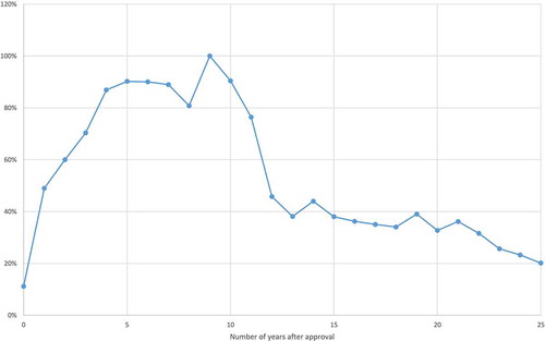
The expression exp(π_n – π₉) is a ‘relative utilization index’: it is the mean ratio of the quantity of a cancer drug sold n years after it was approved to the quantity of the same drug sold 9 years after it was approved.

Estimates of the ‘relative utilization index’ are shown in Figure A2. These estimates indicate that it takes about 9 years for a cancer drug to attain its peak level of utilization. The number of standard units 9 years after FDA approval is about twice as great as the number of standard units one year after FDA approval. Moreover, Figure A2 provides a conservative estimate of the slope of the age-utilization profile, because there was zero utilization of some molecules in the first few years after they were first listed.²¹

Appendix 3.

Table A1. U.S. sales of top cancer drugs ($ millions).

Molecule	2010	2011	2012	2013	2014
All cancer drugs	$21,385	$22,413	$23,299	$24,942	$28,971
RITUXIMAB	$2,673	$2,879	$3,037	$3,199	$3,351
BEVACIZUMAB	$2,993	$2,581	$2,543	$2,618	$2,790
IMATINIB	$1,363	$1,560	$1,674	$1,872	$2,333
DENOSUMAB	$27	$478	$932	$1,229	$1,552
ABIRATERONE ACETATE	$0	$174	$454	$767	$1,010
LENALIDOMIDE	$311	$431	$537	$528	$974
EVEROLIMUS	$108	$182	$426	$714	$841
DASATINIB	$185	$291	$380	$549	$725
LEUPRORELIN	$631	$650	$639	$651	$692
IPILIMUMAB	$0	$339	$507	$541	$687

Source: IMS Health.

these figures represent the value of drugs sold at ‘list prices’; rebates are not accounted for.

Table A2. Data on premature mortality, incidence, and hospitalization, by cancer site.

	Potential years of life lost before age 75		Potential years of life lost before age 65		Average annual number diagnosed before age 75 (SEER 9)		Mean age at diagnosis of patients diagnosed before age 75 (SEER 9)		Number of hospital days
	1999	2014	1999	2014	1988–1997	2003–2012	1988–1997	2003–2012	1997	2013
C00-C14 Head and Neck Cancer	74,052	87,161	34,112	36,161	2,166	2,849	58.0	57.2	159,120	139,442
C15 Esophageal Cancer	99,905	121,933	40,205	45,788	821	959	62.1	61.6	132,260	103,241
C16 Stomach (Gastric) Cancer	95,716	94,763	43,796	43,253	1,199	1,449	61.4	59.7	262,018	199,976
C18 Colon Cancer	286,278	301,178	116,093	129,363	5,376	5,265	62.7	60.1	1,044,400	689,071
C20 Rectal Cancer	48,443	60,020	21,343	26,350	1,710	2,110	61.1	57.5	364,882	268,129
C22 Liver Cancer	109,239	220,317	49,824	83,537	869	2,245	59.3	58.6	81,381	141,369
C25 Pancreatic Cancer	194,392	269,310	75,797	96,095	1,627	2,508	62.8	61.7	276,671	265,989
C34 Lung Cancer	1,089,130	1,010,583	393,295	336,483	10,884	10,652	63.0	62.9	1,183,100	829,940
C40-C41 Bone Cancer	26,401	29,409	18,501	19,729	250	292	35.3	37.8	36,229	42,784
C43 Melanoma	88,005	85,268	47,315	40,233	3,634	5,515	50.5	53.7	15,321	11,540
C44 Basal Cell Carcinoma	15,193	19,996	6,528	7,616	291	439	50.0	53.4	28,348	27,511
C45 Malignant Mesothelioma	14,113	12,243	4,843	4,103	153	138	62.8	63.2	18,289	14,035
C46 Kaposi Sarcoma	590	570	435	345	262	170	39.1	43.0	1,439	0
C49 Soft Tissue Sarcoma	49,563	61,264	29,373	34,339	521	719	46.5	48.9	51,342	58,920
C50 Breast Cancer	427,324	401,888	214,099	186,728	14,100	17,705	56.6	56.4	326,240	157,356
C51 Vulvar Cancer	3,385	6,000	1,435	2,530	205	266	57.0	57.2	18,898	10,365
C53 Cervical Cancer	72,735	70,125	43,145	39,890	1,108	930	46.4	47.6	91,193	39,409
C54.1 Endometrial Cancer	19,773	31,253	7,393	11,158	2,429	3,837	58.6	58.5	159,234	100,397
C56 Ovarian, Fallopian Tube, or Primary Peritoneal Cancer	115,547	115,525	51,707	48,060	1,454	1,548	56.3	55.9	188,761	156,756
C60 Penile Cancer	1,565	2,388	690	1,038	56	87	60.2	60.4	3,157	4,730
C61 Prostate Cancer	76,492	83,051	16,342	20,171	12,716	14,350	65.7	62.9	389,198	153,372
C62 Testicular Cancer	12,311	12,710	8,836	9,110	731	852	34.2	34.9	9,287	12,436
C64-C65 Kidney (Renal Cell) Cancer	92,658	103,563	40,028	40,348	1,990	3,796	58.0	57.7	210,836	229,344
C67 Bladder Cancer	49,151	60,795	16,286	19,515	3,059	3,602	62.7	62.7	244,471	191,431
C69.2 Retinoblastoma	422	205	257	110	21	26	4.9	3.7	381	895
C71 Brain Tumors	176,630	199,026	97,895	101,896	1,291	1,546	45.9	46.9	223,031	221,945
C73 Thyroid Cancer	9,078	12,773	3,968	5,113	1,605	4,281	44.5	47.7	45,057	46,112
C74.9 Neuroblastoma	9,095	8,178	5,645	4,918	35	37	21.4	17.8	14,985	13,315
C81 Hodgkin Lymphoma	26,015	15,628	17,000	9,463	683	744	36.1	38.0	41,761	44,139
C82-C85 Non-Hodgkin Lymphoma	170,143	121,130	79,183	50,615	3,439	4,171	54.6	56.4	456,126	386,511
C90 Multiple Myeloma and Other Plasma Cell Neoplasms	62,555	63,338	22,540	20,973	882	1,370	62.3	61.2	162,886	213,160
C91.0 Acute Lymphoblastic Leukemia (ALL)	33,325	31,268	23,035	20,743	326	446	19.7	22.0	113,448	156,189
C91.1 Chronic Lymphocytic Leukemia (CLL)	16,876	13,585	5,101	4,065	668	1,157	62.8	62.2	47,874	32,660
C91.4 Hairy Cell Leukemia	610	360	275	120	73	89	54.7	54.3	0	0
C92.0 Acute Myeloid Leukemia (AML)	66,432	77,876	35,282	36,561	495	710	53.0	54.3	248,775	390,516
C92.1 Chronic Myelogenous Leukemia (CML)	22,590	7,940	13,065	4,145	240	329	52.0	51.4	54,344	33,370

Table A3. Observed and expected 5-year survival rates and number of patients diagnosed, by cancer site, 2000 and 2008.

	Observed 5-year survival rate		Expected 5-year survival rate		Number of patients diagnosed
Cancer site	2000	2008	2000	2008	2000	2008
C15 Esophageal Cancer	13.5%	14.1%	86.2%	88.0%	2,754	2,994
C16 Stomach (Gastric) Cancer	18.8%	26.0%	83.9%	86.2%	5,055	4,972
C18 Colon Cancer	50.6%	54.6%	80.7%	83.9%	22,409	21,575
C20 Rectal Cancer	54.7%	59.4%	85.6%	89.1%	9,208	8,998
C22 Liver Cancer	10.4%	16.5%	90.8%	91.6%	3,149	5,253
C25 Pancreatic Cancer	4.2%	6.3%	86.2%	88.6%	6,663	8,226
C34 Lung Cancer	12.6%	15.2%	86.2%	86.6%	38,808	38,678
C40-C41 Bone Cancer	66.4%	68.0%	96.1%	96.7%	619	691
C43 Melanoma	81.1%	82.2%	90.1%	89.7%	10,889	13,949
C45 Malignant Mesothelioma	5.0%	8.3%	80.7%	87.4%	647	653
C49 Soft Tissue Sarcoma	59.4%	58.7%	91.0%	91.2%	1,927	2,295
C50 Breast Cancer	79.5%	81.8%	90.0%	91.4%	45,901	47,537
C51 Vulvar Cancer	65.4%	60.0%	86.0%	86.7%	737	778
C53 Cervical Cancer	68.1%	65.0%	95.8%	96.5%	3,557	3,248
C56 Ovarian, Fallopian Tube, or Primary Peritoneal Cancer	40.3%	43.4%	92.1%	93.0%	4,869	5,014
C60 Penile Cancer	61.4%	57.1%	82.3%	83.8%	246	258
C61 Prostate Cancer	80.6%	85.2%	81.9%	86.4%	49,820	53,557
C62 Testicular Cancer	94.2%	94.4%	98.5%	98.4%	2,049	2,237
C64-C65 Kidney (Renal Cell) Cancer	56.9%	66.6%	88.3%	90.0%	7,148	10,573
C67 Bladder Cancer	62.6%	62.8%	80.3%	81.4%	11,874	12,633
C69.2 Retinoblastoma	78.7%	76.2%	89.4%	90.5%	557	562
C71 Brain Tumors	28.9%	29.9%	97.2%	97.2%	4,084	4,520
C73 Thyroid Cancer	92.2%	93.9%	96.1%	96.1%	5,170	9,228
C81 Hodgkin Lymphoma	81.2%	84.9%	97.1%	96.9%	1,931	2,170
C82-C85 Non-Hodgkin Lymphoma	54.6%	62.4%	88.0%	88.6%	11,964	13,585
C90 Multiple Myeloma and Other Plasma Cell Neoplasms	28.9%	42.4%	85.5%	87.4%	3,644	4,241
C91.0 Acute Lymphoblastic Leukemia (ALL)	62.3%	66.5%	99.1%	99.1%	1,145	1,311
C91.1 Chronic Lymphocytic Leukemia (CLL)	64.0%	68.3%	81.9%	83.1%	2,550	3,153
C92.0 Acute Myeloid Leukemia (AML)	16.6%	23.6%	94.8%	95.3%	2,303	2,454
C92.1 Chronic Myelogenous Leukemia (CML)	45.5%	57.0%	90.6%	90.9%	1,100	1,209

Table A4. Calculation of the cost per life-year gained in 2014 from cancer drugs approved during 2000–2014.

Line	Description	Basis	Value
(1)	Total expenditure (before rebates) on cancer drugs in 2014	IMS Institute for Healthcare Informatics (2015)	$32,300,000,000
(2)	Fraction of total expenditure on post-1999 drugs	Author’s calculations based on IMS MIDAS data	67.7%
(3)	Expenditure (before rebates) on post-1999 cancer drugs in 2014	(1) * (2)	$21,867,100,000
(4)	Rebates on post-1999 drugs, assuming 25% rebate rate (Herper (2012))	25% * (3)	$5,466,775,000
(5)	Reduction in old drug cost (assumed to be 25% of new drug cost) (Lichtenberg (2014c))	25% * ((3) – (4))	$4,100,081,250
(6)	Hospital cost reduction	Author’s calculations based on estimates of models 1 and 5 in Table 6.	$4,770,000,000
(7)	Net expend–all ages	(3) – ((4) + (5) + (6))	$7,530,243,750
(8)	Net expend–below age 75 (assumed to be 75% of net expenditure for all ages)	75% * (7)	$5,647,682,813
(9)	Life-years before age 75 gained, controlling for incidence and mean age at diagnosis	Author’s calculations based on estimates of models 1 and 2 in Table 5a.	719,133
(10)	Cost per life-year gained before age 75	(9)/(8)	$7,853

Figure A1. Number of cancer and other new molecular entities launched worldwide, 1982–2015.

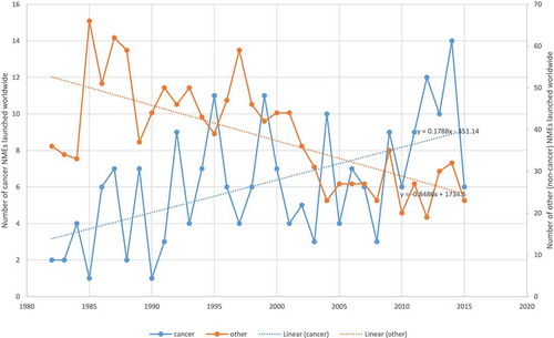
Figure A2. Mean ratio of the quantity of a cancer drug sold n years after approval to the quantity of the same drug sold 9 years after approval.

References

- National Cancer Institute. Drugs approved for different types of cancer. [ cited 2019 Dec 7]. Available from: https://www.cancer.gov/about-cancer/treatment/drugs/cancer-type
- Food and Drug Administration. Drugs@FDA database. [ cited 2019 Dec 7]. Available from: https://www.fda.gov/drugs/drug-approvals-and-databases/about-drugsfda
- Food and Drug Administration. Review designation policy: priority (P) and standard (S). 2019 [cited 2019 Dec 7]. Available from: https://www.fda.gov/media/72723/download
- National Cancer Institute. Cancer screening overview. [ cited 2019 Dec 7]. Available from: https://www.cancer.gov/about-cancer/screening/hp-screening-overview-pdq
- Ederer F, Axtell LM, Cutler SJ. The relative survival rate: a statistical methodology. Natl Cancer Inst Monogr. 1961;6:101–121.
- Centers for Disease Control and Prevention. Compressed mortality database. [ cited 2019 Dec 7]. https://wonder.cdc.gov/mortSQL.html
- National Cancer Institute. SEER research data. [ cited 2019 Dec 7]. Available from: https://seer.cancer.gov/data/
- National Cancer Institute. SEER• Stat Software. [ cited 2019 Dec 7]. Available from: https://seer.cancer.gov/seerstat/
- Agency for Healthcare Research and Quality. HCUPnet: A tool for identifying, tracking, and analyzing national hospital statistics. [ cited 2019 Dec 7]. Available from: https://hcupnet.ahrq.gov/#setup
- Centers for Disease Control and Prevention. WISQARS years of Potential Life Lost (YPLL) Report, 1999 and later. [ cited 2019 Dec 7]. Available from: https://webappa.cdc.gov/sasweb/ncipc/ypll10.html
- IMS Institute for Healthcare Informatics. Medicines use and spending shifts: a review of the use of medicines in the U.S. in 2014. Parsippany NJ: IMS Institute for Healthcare Informatics. 2015 Apr.
- Herper M Inside the secret world of drug company rebates. Forbes. 2012 May 10.
- Lichtenberg FR. The impact of pharmaceutical innovation on disability days and the use of medical services in the United States, 1997–2010. J Hum Capital. 2014 Winter;8(4):432–480.
- Hirth RA, Chernew ME, Miller E, et al. Willingness to pay for a quality-adjusted life year: in search of a standard. Med Decis Making. 2000 Jul-Sep;20(3):332–342.
- World Health Organization. Cost-effectiveness thresholds. [ cited 2019 Dec 7]. Available from: https://www.who.int/bulletin/volumes/94/12/15-164418/en/
- Lichtenberg FR. The impact of new drug launches on life-years lost in 2015 from 19 types of cancer in 36 countries. J Demographic Econ. 2018;84(3):309–354.
- Cressman S, Browman GP, Hoch JS, et al. A time-trend economic analysis of cancer drug trials. Oncologist. 2015 Jul;20(7):729–736. [cited 2019 Dec 7]. Available from: https://www.ncbi.nlm.nih.gov/pmc/articles/PMC4492232/
- Wieseler B, McGauran N, Kaiser T. New drugs: where did we go wrong and what can we do better?. BMJ. 2019;366.doi: 10.1136/bmj.I4340
- Davis C, Naci H, Gurpinar E, et al. Availability of evidence of benefits on overall survival and quality of life of cancer drugs approved by European Medicines Agency: retrospective cohort study of drug approvals 2009-13. BMJ. 2017;359:j4530.
- Pease AM, Krumholz HM, Downing NS, et al. Postapproval studies of drugs initially approved by the FDA on the basis of limited evidence: systematic review. BMJ. 2017;357:j1680.
- Gyawali B, Hey SP, Kesselheim AS. Assessment of the clinical benefit of cancer drugs receiving accelerated approval. JAMA Intern Med. 2019;179:906. [Epub ahead of print.].
- Martin M. The Cambridge companion to Atheism. Cambridge companions to philosophy. Cambridge, UK: Cambridge University Press; 2007.
- Alderson P. Absence of evidence is not evidence of absence. BMJ. 2004;328(7438):476–477.
- Lichtenberg FR. How many life-years have new drugs saved? A 3-way fixed-effects analysis of 66 diseases in 27 countries, 2000–2013. Int Health. 2019 Sep;11(5):403–416.
- Lichtenberg FR. The impact of access to prescription drugs on disability in eleven European countries. Disabil Health J. 2019 Jul;12(3):375–386.
- Frieden TR. Evidence for health decision making — beyond randomized, controlled trials. N Engl J Med. 2017 Aug 3;377:465–475. [cited 2019 Dec 7]. Available from: https://www.nejm.org/doi/full/10.1056/NEJMra1614394
- Booth CM, Tannock IF. Randomised controlled trials and population-based observational research: partners in the evolution of medical evidence. Br J Cancer. 2014 Feb 04;110:551–555. [cited 2019 Dec 7]. Available from: https://www.nature.com/articles/bjc2013725
- Deaton A, Cartwright N. Understanding and misunderstanding randomized controlled trials. Soc Sci Med. 2018;210:2–21. Available from: http://www.sciencedirect.com/science/article/pii/S0277953617307359
- Nordhaus WD. Irving Fisher and the contribution of improved longevity to living standards. Am J Econ Sociology. 2005 Jan;64(1):367–392.
- United Nations. Human Development Index (HDI) | Human development reports. 2017 Dec 7. Available from: hdr.undp.org/en/content/human-development-index-hdi
- Grossman GM, Helpman E. Innovation and growth in the global economy. Cambridge (MA): MIT Press; 1991.
- Romer PM. Endogenous technological change. J Political Econ. 1990 Oct;98(5, Pt. 2):S71–S102.
- Aghion P, Howitt P. A model of growth through creative destruction. Econometrica. 1992 Mar;60(2):323–351.
- Jones CI. Sources of U.S. Economic growth in a world of ideas. Am Econ Rev. 2002 Mar;92(1):220–239.
- Patterson GS. The business of ideas: the highs and lows of inventing and extracting revenue from intellectual property. AuthorHouse, Bloomington, IN; 2012 Sep 14.
- Lichtenberg FR. The effect of pharmaceutical innovation on longevity: patient level evidence from the 1996–2002 medical expenditure panel survey and linked mortality public-use files. Forum Health Econ Policy. 2013 Jan;16(1):1–33.
- Lichtenberg FR. Pharmaceutical innovation and longevity growth in 30 developing and high-income countries, 2000–2009. Health Policy Technol. 2014 Mar;3(1):36–58.
- Dorsey ER, de Roulet J, Thompson JP, et al. Financial anatomy of biomedical research, 2003–2008. J Am Med Assoc. 2010;303(2):137–143.
- Sampat BN, Lichtenberg FR. What are the respective roles of the public and private sectors in pharmaceutical innovation? Health Affairs. 2011;30(2):332–339.
- National Cancer Institute. Enhancing drug discovery and development. [ cited 2019 Dec 7]. Available from: https://www.cancer.gov/research/areas/treatment/enhancing-drug-discovery
- Lichtenberg FR. The impact of pharmaceutical innovation on longevity and medical expenditure in France, 2000–2009. Econ Hum Biol. 2014 Mar;13:107–127.
- Burnet NG, Jefferies SJ, Benson RJ, et al. Years of life lost (YLL) from cancer is an important measure of population burden – and should be considered when allocating research funds. Br J Cancer. 2005 Jan 31;92(2):241–245.
- Broda C, Weinstein DW. Variety growth and World Welfare. Am Econ Rev. 2004;94(2):139–144.
- National Cancer Institute. Long-term trial results show no mortality benefit fromannual prostate cancer screening. 2012 Feb 17 [cited 2019 Dec 7]. Available from: https://www.cancer.gov/types/prostate/research/screening-psa-dre
- Food and Drug Administration. Real world evidence. [ cited 2019 Dec 7]. Available from: https://www.fda.gov/science-research/science-and-research-special-topics/real-world-evidence
- National Science Foundation. U.S. Corporate R&D: volume 1: top 500 Firms in R&D by Industry Category. 2016 [cited 2019 Dec 7]. Available from: http://wayback.archive-it.org/5902/20150819114914/http:/www.nsf.gov/statistics/nsf00301/expendit.htm#intensity