The influence of product instability on slow-binding inhibition

Abstract

We present a kinetic study of an enzyme reaction that takes place with slow-binding inhibition where the immediate product undergoes a spontaneous or induced process of decomposition. A kinetic study of an enzyme process, in which a slow-binding inhibition process and a decomposition of the immediate product of the reaction take place simultaneously is performed. The corresponding explicit concentration-time equations were obtained. Using the analytical solutions obtained, which were tested numerically, we suggest a procedure that allows the discrimination between the particular cases considered and the evaluation of the principal kinetic parameters of the reaction.

Keywords::

• Enzyme inhibition
• enzyme reactions
• rapid equilibrium
• slow-binding inhibition
• unstable product
• enzyme kinetics

1 Introduction

Enzyme reactions exist, in which the product instability influences the evaluation of the kinetic parameters 1-6. Enzyme reactions, in which the products are unstable and undergo a chemical decomposition, deprotonation or other destabilization by first- or second-order kinetics, have been described previously 1-6. The case of an unstable product has been exemplified by the kinetic study of the oxidation of 3,4-dihydroxyphenylethylamine (dopamine) to the corresponding o-quinone catalyzed by the enzyme tyrosinase (monophenol, dihydroxy-l-phenylalanine: oxygen oxido-reductase, EC 1.14.18.1) (Garrido et al.) [7]. It has been shown that the direct product of the enzyme catalysis is o-dopamine-quinone-, which is converted non-enzymatically to o-dopamine-chrome by the cyclization of the molecule following a Michael intramolecular 1,4-addition.

Kinetic analysis of enzyme reactions, in which processes of slow-binding inhibition take place, have often been reported in the literature 8-11. In some cases the inhibitor and the enzyme interact slowly; in others, an enzyme-inhibitor complex, which is formed by a slow isomerization, is formed rapidly. Examples are the inhibition of the catecholase activity of grape polyphenol oxidase by tropolone [12] or the inhibition by 3-hydroxy-4-phenylthiazole-2 (3H)-thione (3H4PTT) of dopamine beta-monooxygenase (DbetaM) [13]. The slow-binding inhibition of jack bean urease by 1,4-benzoquinone (BQ) and 2,5-dimethyl-1,4-benzoquinone (DMBQ) has recently been studied [14]. Sometimes, a single species (the free enzyme, the substrate, the enzyme-substrate complex, an inhibitor or the product of the reaction) is unstable [15].

In previous work on the slow-binding inhibition of tyrosinase of frog epidermis by m-cumaric acid [16], the reaction was monitored by measuring the accumulated final product in the reaction media (dopachrome) which is formed from the corresponding o-quinone generated by the enzyme in its action on l-dopa. In this case the kinetic analysis made was very simple corresponding to only one exponential term in the time course equation used. To obtain the experimental results it was conducted at in order that the apparent rate constant corresponding to the transformation of o-dopaquinone reaches a high value in comparison with the time-dependent inhibition, so that the transient phase was controlled by this latter process. Nevertheless, at lower pH-values both processes overlap in time and in these situations, at the present relatively seldom, it a new and more complete kinetic analysis is necessary which allows the carrying out of these type of studies.

In this paper, a kinetic analysis of a Michelis-Menten mechanism is carried out in which a slow-binding inhibition process occurs and, moreover, the immediate product is unstable. We assumed an initial steady-state in the catalytic route and a reversible reaction step, in which the free enzyme and the enzyme-substrate complex rapidly reach equilibrium, and studied the progress curve of the product, P, generated directly by the enzyme, as well as that one corresponding to the compound, R, obtained from P. Subsequently, we evaluated the kinetic parameters of the reaction. A numerical example was outlined and solved to demonstrate the quality of the method suggested. The results have been compared with those obtained by the numerical solution of the differential equations that describe the kinetics of the process.

2 Theory

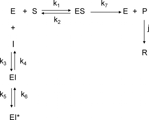
The general mechanism studied in this paper is shown in Scheme 1.

short-legendScheme 1

2.1 Notation and definitions

Equation (A1) of the Appendix describes the kinetics of Scheme 1. This equation does not admit any analytical solution, but approximate solutions can be derived, if one assumes that: In this case:

After the insertion of equation (2) into equation (A1) of the Appendix, the latter becomes linear and has, therefore, analytical solutions. The explicit equations for the concentrations of P and R are: and where λ_h (always negative or complex with a negative real part) are the eigenvalues of the coefficients matrix of equation (A1) of the Appendix, i.e., the roots of the equation: The corresponding expressions of the coefficients of equation (5) are given in the Appendix.

If we assume a pseudo steady-state 17-21 from the onset of the reaction in the catalytic route then: In this case, taking equations (6) and 11-A16 into account, equation (5) can be written:

According to equations (6) and 17-A20 of Appendix, and, therefore, the term of equations (3) and (4) containing the parameter λ₃ can be neglected. The latter will have only three exponential terms: − j, λ₁ and λ₂.

2.2 Particular cases:

1. In some cases the formation of the enzyme-inhibitor complex, EI, is very fast and is followed by a slow isomerization to EI* [10]; then, assuming conditions of rapid equilibrium, we have: In this case, it can be demonstrated easily that and that the term of the explicit equation of the product P or R containing λ₂ can be neglected. Therefore, if we set the corresponding equations for [P] and [R] will be: The parameters of these equations are given in the Appendix.

2. In the case in which the eigenvalues of the corresponding matrix of coefficients of equation (1) are the roots of the equation: where H₁ and H₂ are given in Appendix

According to the condition expressed by equation (6) and the polynomial properties, equation (11) can be written: where i.e., and, therefore, the explicit equations for [P] and [R] will have only two exponential terms, those ones involving in their exponents − j and λ₁, i.e. they will have the same form as equations (9) and (10).

3. In the case that the slow transition corresponds only to the inhibition and the explicit equations for [P] and [R] are: where λ, [P]_∞ and γ are given by equations (A28), (A29) and (A40, respectively.

3 Materials and methods

The simulated progress curves have been obtained by numerical solution [22] of the corresponding system of differential equations using a set of arbitrary, but realistic values of the initial concentrations and the rate constants. The simulated errors with the mean of 0 and a specified S.D. were added using a random normal distribution based on the algorithm of Box, Muller and Marsaglia [23] and a computer program. The analytical solutions of the system of differential equations were obtained by the Laplace transformation. The regressions were performed using the software SigmaPlot for Windows 4.0 of Jandel Scientific in a personal computer equipped with an Intel Pentium III/850 MHz processor. The enzyme reaction was always started by the addition of the enzyme to a mixture of the substrate and the inhibitor.

4 Results and discussion

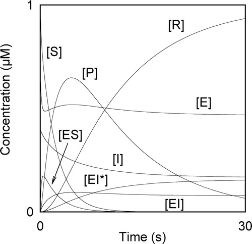
We have obtained the explicit equations for the formation of the product (P) of an enzyme reaction and the one of the accumulation of composed (R) that is originated from P in which a slow-binding inhibition process proceeds according to Scheme 1, assuming that the initial concentrations of the substrate and the inhibitor are much higher than that of the free enzyme (to ensure that the concentrations of the substrate and the inhibitor remain practically constant) and that a very fast formation occurs of the enzyme-inhibitor complex, EI, which is followed by a slow isomerization to an EI* complex. Figure 1 shows the time progress curves of all of the species of Scheme 1. They were plotted using the numerical solutions of the set of differential equations that describes the kinetics of Scheme 1. Note that the progress curve of P has a maximal value, [P]_max. The corresponding value of the time, t_max, can be easily determined experimentally. The progress curve of the product reaches an inflexion point, [P]_inflex, at . The t_max- and t_inflex-values can be evaluated from the plot of d[P]/dt vs. time. The period of time elapsing to t_max, at which t_∞, can be useful, since it allows the evaluation of [P]_∞ without reaching the end of the reaction, i.e. the [P]_∞-value can be obtained from t_max and t_inflex. If we denote the following quotient with q: then it is easily demonstrated that if the curve is described by an equation such as equation (9), i.e. when the corresponding explicit equation has only two exponential terms. If λ does not vary linearly with [I]₀, then, according to equation (A28), the mechanism is compatible with that of case 1. If λ varies linearly with [I]₀, then, according to equation (A38), the particular case 2 is suitable. In the case in which j has a high value (case 3) the accumulation of P and R takes place according to a uniexponential equation, as was shown in the case of the slow inhibition of tyrosinase of frog epidermis by m-cumaric acid at [16].

Figure 1 Progress curves of the species involved in Scheme 1 obtained by numerical solution of the set of differential equations that describes the kinetics of the enzyme system. The arbitrary values used for the initial concentrations and rate constants are: , ,

4.1 Kinetic analysis

The kinetic analysis suggested in this paper allows the evaluation of the kinetic parameters of the reaction described by Scheme 1 and the discrimination between the particular cases presented. This analysis is based on the progress curve of the product P or on the progress curve of the species R which the immediate product is transformed into. Next we summarize this procedure.

4.1.1 Analysis based on the experimental progress curve of the product (P)

For different values of the initial concentrations of the substrate and the inhibitor fulfilling the conditions indicated in the Theory section, we obtain progress curves of the product and the corresponding curves for the first derivative. For each curve, the values of [P]_∞, [P]_max, [P]_inflex, t_∞, t_max, t_inflex and α₀ are obtained as is described below. Each curve of P is fitted at sufficiently long times (> t_max) to a uni-exponential equation. From the plot of vs. time, we obtain one of the non-linear parameters of equation (9) and the corresponding linear parameter. With the t_max- or t_∞-values, equations (A34) (or (A35)) permit the evaluation of the remaining parameters of equation (9). The non-linear parameter, which does not depend on the concentrations, will be the j-value. If λ varies linearly with [I]₀, then, according to equation (A38), the particular case 2 may be considered.

From the plot of d[P]/dt vs. t, data points, which are located near the are chosen. These points are fitted using a polynomial of the type by the least-squares approximation. The polynomial fitting can be carried out with the Chebyshev polynomials [24] or the Marquardt algorithm [25]. Commercial software packages for the personal computer as SigmaPlot^© (Jandel Scientific), MathCad^© (MathSoft Inc., Cambridge, MA), Maple^© (Waterloo Maple Software, Waterloo, Ontario, Canada), Derive^© (Soft Warehouse) can be used. Once the coefficients of polynomial have been determined, the t_max-value is obtained by solving the equation The [P]_max-value can be evaluated by setting in equation (9) or by solving the equation obtained after fitting to a polynomial of the degree three of the points near [P]_max. The plot of d[P]/dt vs. t exhibits a minimum value that allows the evaluation of the t_inflex-value. If a set of data points near this minimum is fitted to a polynomial f(t) of the degree three, then the t_inflex-value will be one of the roots of equation i.e. one of the roots of the equation (see Figure 2a). Following a similar procedure, the t_∞-value can be obtained by fitting the data points near [P]_∞ of [P] vs. t to a polynomial of the degree two and solving the equation (see Figure 2b). The value of f(t) at i.e. α₀, can be obtained by fitting to a polynomial of degree two of a set of points of d[P]/dt vs. t located at short time values. Once the polynomial has been obtained, the independent term, i.e. the value for will be equal to α₀ (see Figure 2c). At longer time values, the parameter q can be evaluated as described above. equation (A32) allows us to evaluate the constant k₆. According to equation (A31), the plot of [E]₀/α₀ vs. 1/[S]₀ gives at constant [I]₀ a straight line with an ordinate intercept equal to 1/k₇. The plot of ([S]₀[E]₀)/(j[P]_∞) against [I]₀ yields at constant [S]₀ according to equation (A29) a straight line with ordinate intercept and slope K_m(k₅+k₆)/(K_Ik₆k₇). According to equation (A31), the plot of ([S]₀[E]₀)/(α₀) vs. [I]₀ at constant [S]₀ gives a straight line of slope K_m/(K_Ik₇). The quotient between the two slopes yields

Figure 2 (a) Evaluation of t_inflex. A set of points with low values of d[P]/dt are chosen. These points are fitted using a polynomial of degree three. One root of the derivative of this polynomial is t_inflex. (b) Evaluation of t_∞. Data points at t < t_max, which are located near are chosen. These points are fitted using a polynomial of the degree two. One root of the equation is t_∞. (c) Evaluation of α₀. The first data points of d[P]/dt, i.e. data points at low t-values, are fitted using a polynomial of the degree two. The independent term of this polynomial is α₀.

4.1.2 Analysis based on the experimental progress curve of the species R

The analysis of the experimental results is made in a similar form to that described previously for the product. A simplified kinetic analysis was carried out experimentally in a study of m-cumaric acid acting as slow inhibitor of frog epidermis tyrosinase [16], working at a pH adopted, so that j was much greater than k₅ and k₆. At lower pH values the dependence of [R] on t would correspond to a biexponential equation (10).

4.2 Numerical example

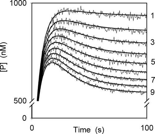
To illustrate the procedure suggested here, we chose a numerical example in which we obtain simulated curves (shown in Figure 3) by numerical integration of the differential equations (equation (A1) of the Appendix) describing the behaviour of the enzyme system using the arbitrary set of values of the rate constants and initial concentrations listed in the legend to Figure 3. Then, the simulated progress curves are used as if they were experimental progress curves. The values used in the simulations fulfil the condition established in the Theory section. Simulated experimental errors with an S.D. of 1% were added as indicated in the Materials and Methods section. Two sets of curves we obtained, one at constant [S]₀ (and varying [I]₀) and another at constant [I]₀ (and varying [S]₀).

Figure 3 Progress curves simulated with added errors and calculated (continuous lines) using equation (9) corresponding to the proposed example. The values of the rate constants and initial concentrations used are: for the curves 1–9, respectively.

We proceeded as indicated above with curve 9 of Figure 3, in which the initial concentrations for enzyme, substrate and inhibitor were and resp. The values obtained for t_max, t_inflex and t_∞ are 17.60 s, 28.61 s and 6.64 s, resp. (see Figures 2a and 2b). In this case, the parameter q is equal to 1.005, which shows the bi-exponential shape of the progress curve. The α₀-value was (see Figure 2c). With the [P]_∞-value the equation (A34) and the plot of vs time, we obtained for λ, j and A₀ the values − 0.0469 s^{− 1}, 0.1585 s^{− 1}, resp. In this case λ does not vary linearly with [I]₀, and, according to equation (A28) the mechanism is compatible with that of case 2. Following the procedure indicated above, according to equation (A31) the plot of [E]₀/α₀ against 1/[S]₀ gives at constant [I]₀ a straight line with ordinate intercept (1/k₇) (see Figure 4). The plot of ([S]₀[E]₀)/(j[P]_∞) against [I]₀, at constant [S]₀, gives a straight line with the ordinate intercept and the slope (see Figure 5). According to equation (A31), the plot of ([S]₀[E]₀)/(α₀) vs. [I]₀ gives at constant [S]₀ a straight line of slope {K_m/(K_Ik₇)} The quotient between the latter two slopes yields

Figure 4 (a) Plot of [E]₀/(j[P]_∞) vs. 1/[S]₀ at constant [I]₀ according to equation (A29). (b) Plot of [E]₀/α₀ vs. 1/[S]₀ at constant [I]₀ according to equation (A31).

Figure 5 (a) Plot of ([S]₀[E]₀)/(j[P]_∞) vs. [I]₀ at constant [S]₀ according to equation (A29). (b) Plot of ([S]₀[E]₀)/α₀ vs. [I]₀ at constant [S]₀ according to equation (A31).

With these results and equation (A32), we have obtained for the kinetic parameters k₅, k₆, k₇, j, K_m and K_I the values and respectively.

[E]:	=	Enzyme concentration
[E]0:	=	Initial enzyme concentration
[S]:	=	Substrate concentration
[S]0:	=	Initial substrate concentration
[I]:	=	Inhibitor concentration
[I]0:	=	Initial inhibitor concentration
[ES]:	=	Concentration of the enzyme-substrate complex
[EI], [EI*]:	=	Concentrations of the enzyme-inhibitor complexes
[P]:	=	Product concentration
[R]:	=	Concentration of the species into which P is transformed
[P]∞:	=	Concentration of P obtained at the final stage of the reaction
[P]max:	=	Maximal value of [P]
[P]inflex:	=	[P] corresponding to the inflexion point of the progress curve of P
tmax:	=	Time corresponding to [P]max
tinflex:	=	Time corresponding to [P]inflex
t∞:	=	Time elapsing to tmax at which
Km:	=	Michaelis constant,
KI:	=	Equilibrium constant, k4/k3

Acknowledgements

This work was partially supported by the Dirección General de Enseñanza Superior e Investigación Científica (Plan Nacional de Investigación Científica) Project Number BQU2002-01960 and by the Dirección General de Investigación e Innovación (Consejería de Ciencia y Tecnología de la Junta de Comunidades de Castilla-La Mancha) Grupo Consolidado Number GC-02-032.

Appendix

Matricial equation that describes the kinetics of the species in Scheme 1 There are the following mutual relationships: The coefficients F₁, F₂ and F₃ of equation (5) are given by the equations 11-A13 resp. According to polynomial properties and equation (6) and: Equation (A18) readily yields:

Particular case 1:

According to equations (8) and 11-A13 we can write: where, according to polynomial properties:

Particular case 2

Coefficients of equation (11):

Particular case 3

References

- García-Carmona F, García-Cánovas F, Iborra JL, Lozano JA. Kinetic study of the pathway of melanization between L-dopa and dopachrome. Biochim Biophys Acta 1982; 717: 124–131
- Escribano J, García-Cánovas F, García-Carmona F, Lozano JA. Kinetic study of the transient phase of a second-order chemical reaction coupled to an enzymic step: Application to the oxidation of chlopromazine by peroxidase-hydrogen peroxide. Biochim Biophys Acta 1985; 831: 313–320
- Escribano J, Garcia-Carmona F, Garcia-Canovas F, Iborra JL, Lozano JA. Kinetic analysis of chemical reactions coupled to an enzymic step. Application to acid phosphatase assay with Fast Red. Biochem J 1984; 223(3)633–638
- Jiménez M, Garcia-Canovas F, Garcia-Carmona F, Lozano JA, Iborra JL. Kinetic study and intermediates identification of noradrenaline oxidation by tyrosinase. Biochem Pharmacol 1984; 33(22)3689–3697
- Jimenez M, Garcia-Carmona F, Garcia-Canovas F, Iborra JL, Lozano JA, Martinez F. Chemical intermediates in dopamine oxidation by tyrosinase, and kinetic studies of the process. Arch Biochem Biophys 1984; 235(2)438–448
- Escribano J, Garcia-Canovas F, Garcia-Carmona F, Lozano JA. Kinetic study of the transient phase of a second-order chemical reaction coupled to an enzymic step: Application to the oxidation of chlorpromazine by peroxidase-hydrogen peroxide. Biochim Biophys Acta 1985; 831(3)313–320
- Garrido-del Solo C, García-Cánovas F, Havsteen BH, Varón R. Kinetics of an enzyme reaction in which both the enzyme-substrate complex and the product are unstable or only the product is unstable. Biochem J 1994; 303: 435–440
- Morrison JF, Walsh CT. The behavior and significance of slow-binding enzyme inhibitors. Adv Enzymol 1988; 61: 201–301
- Szedlacsek S, Duggleby RG. Kinetics of slow and tight-binding inhibitors. Meth Enzymol 1995; 249: 144–180
- Sculley MJ, Morrison JF, Cleland WW. Slow-binding inhibition: The general case. Biochim Biophys Acta 1996; 1298: 78–86
- Garrido-del Solo C, García-Cánovas F, Havsteen B, Varón R. Kinetic analysis of enzyme reactions with slow-binding inhibition. BioSystems 1999; 51: 169–180
- Valero E, García-Moreno M, Varón R, García-Carmona F. Time-dependent inhibition of grape polyphenol oxidase by tropolone. J Agric Food Chem 1991; 39: 1043–1046
- Dharmasena SP, Wimalasena DS, Wimalasena K. A slow-tight binding inhibitor of dopamine betamonooxygenase: A transition state analogue for the product release step. Biochemistry 2002; 15(41)12414–12420
- Zaborska W, Kot M, Superata K. Inhibition of jack bean urease by 1,4-benzoquinone and 2,5-dimethyl-1,4-benzoquinone. Evaluation of the inhibition mechanism. J Enz Inhib Med Chem 2002; 17: 247–253
- Duggleby RG. Progress curves of reactions catalyzed by unstable enzymes. A theoretical approach. J Theor Biol 1986; 123: 67–80
- Cabanes J, Garcia-Carmona F, Garcia-Canovas F, Iborra JL, Lozano JA. Kinetic study on the slow inhibition of epidermis tyrosinase by m-cumaric acid. Biochim Biophys Acta 1984; 790(2)101–107
- Waley SG. Kinetics of suicide substrates. Biochem J 1980; 185: 771–773
- Tatsunami S, Yago N, Hosoe M. Kinetics of suicide substrates. Steady-state treatments and computer-aided exact solutions. Biochim Biophys Acta 1981; 662: 226–235
- Tsou C-L, Meister A. Kinetics of substrate reaction during irreversible modification of enzyme activity. Adv Enzymol 1988; 61: 381–436
- Topham CM. A generalized theoretical treatment of the kinetics of an enzyme-catalysed reaction in the presence of an unstable irreversible modifier. J Theor Biol 1990; 145: 547–572
- Wang Z-X. Kinetics of suicide substrates. J Theor Biol 1990; 147: 497–508
- García-Sevilla F, Garrido-del Solo C, Duggleby R, García-Cánovas F, Peyró R, Varón R. Use a windows program for simulation of the progress curves of reactants and intermediates involved in enzyme-catalyzed reactions. BioSystems 2000; 54: 151–164
- Rugg T, Feldman P. Turbo pascal biblioteca de programas. Editorial Anaya, Madrid 1987
- Burden R, Faires J. Análisis numérico. Grupo Editorial Iberoamérica, México 1985
- Marquardt DW. An algorithm for least-squares estimation of nonlinear parameters. J Soc Ind Appl Math 1963; 11: 431–441