Simple views on different problems in physics: from drag friction to tough biological materials

Abstract

We discuss the dynamics of bubbles and liquid drops in quasi two dimensions, i.e. in the Hele-Shaw cell, confirming different scaling laws for viscous drag friction, together with scaling laws for a number of related phenomena. Motivated by the study on viscous drag friction, we describe an experiment on drag friction in a granular medium, which reveals a length scale that diverges towards the jamming transition. These examples in the dynamics of viscous fluid and granular materials underscore the importance of the scaling concept in understanding physical phenomena, often vindicated by a clear data collapse by virtue of a corresponding scaling law. To demonstrate the universal usefulness of the strategy, we discuss another different example from the strength of biological materials. To stress a wide applicability of the scaling approach, we introduce the robustness of scaling laws and justify frequent emergence of the robustness.

Keywords:

• scaling laws
• drag friction
• jamming transition
• strength of biological materials

1. Introduction

The scaling concept has been known to be useful in various fields. For example, classic text books of particle physics [1] as well as fracture mechanics [2] start from the discussion on dimensional analysis. The scaling hypothesis in critical phenomena resulted in the birth of renormalization group [3]. However, the scaling approach was not regarded as a strategy that is complete enough to finish any physics studies: it was rather considered as an informal first-step consideration.

The importance of the scaling approach was further put forward by de Gennes, particularly in textbooks of polymers [4] and capillarity [5], to show that the scaling approach could be a physics strategy that is sound enough to finish a physical consideration if the problem in question is complex (at least for physicists). As a result, the scaling approach is now well accepted in the field of soft matter and well used by a relatively small portion of researchers in the field.

However, it has yet to be well used as a standard strategy in various field of physics and for researchers in more application-oriented fields including those in industry, despite of its high potential. Accordingly, to inspire such potential users of the approach, we set the purpose of this paper to provide a variety of examples in which the scaling approach successfully provides a clear physical picture with scaling laws justified by a distinct data collapse.

This article is organized as follows. We start with the problem of viscous drag friction acting on a fluid drop surrounded by another fluid in a confined space in the Hele-Shaw cell. After discussing other examples in which viscous dissipation plays a significant role, we proceed to describe an experiment of granular drag friction in a two-dimensional cell, which was motivated by the study of viscous drag in the Hele-Shaw cell. Finally, we discuss the strength and toughness of biological materials, revealing that the same strategy works effectively to provide some simple views on the mechanical superiority. We summarize various advantages of the scaling approach at the end.

We stress here that the scaling approach is not necessarily limited to rather special cases: scaling laws can be ‘robust.’ Scaling laws are often derived in the limit in which a certain physical parameter is much smaller than a characteristic value , i.e. in the limit of . Because of this, scaling laws tend to be accepted as a formula that is useful only in a very limited or special case, which is not always true, as we exemplified in Section 5.

Since we discuss different problems in a short note, we could not give a detailed background for each topic. Readers who get interested in a specific topic are recommended to return original articles cited in this article, in which they should find a relevant background.

2. Viscous drag friction for a fluid drop in the Hele-Shaw cell

The experimental set-up is shown in Figure 1. The experimental parameters for the rising bubble experiment in Figure 1(a) are specified in Table 1. We measured the transverse and longitudinal diameters and of rising bubbles as defined in Figure 2(a)(1) to obtain Figure 2(b). The results show that the bubble is slightly elongated in the rising direction and, as seen in the inset, the aspect ratio is almost constant for all the parameters we studied. The reason for the observed universal aspect ratio has yet to be explored.

Figure 1. (colour online) Illustration of experiment for a rising bubble (a), and for a sinking drop (b). The Hele-Shaw cell is made up of transparent acrylic plates. The cell thickness is a few millimetres and the size of the bubble or drop is about one centimetre. The width and height of the cell is much larger than the size of the drop.

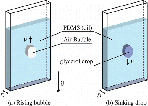
Figure 2. (colour online) (a) Moving fluid drops in a Hele-Shaw cell. Here, the viscosity of the fluid drop and the surrounding fluid are denoted and , respectively. (1) The rising bubble (‘air drop’) is slightly deformed from a circle and characterized by the longitudinal and transverse diameters, and , respectively, as indicated in the photograph. (2) A glycerol drop surrounded by a more viscous oil (as in (1)) is sinking in the cell. The fluid drop shape is very similar to that in (1). (3) A glycerol drop surrounded by a less viscous oil (different from (1) and (2)) is sinking in the cell. Compared with (1) and (2), the elongation is significant. (b) vs. for the bubble experiment. The symbols are specified in Table 1. (c) vs. for the bubble experiment. (d) Plot in (c) replotted with the two axes, the renormalized velocity Ca and the renormalized cell thickness , demonstrating a clear data collapse by virtue of the theory. (e) Plot of Ca vs. , in which the data are not well collapsed as in (d), showing that the factor is important to explain the experiment. Figures are reproduced from [6].

Table 1. Experimental parameters and symbols used in Figures . The densities of PDMS oils with the kinematic viscosities , 500–3000, 5000–10,000 cS are 0.965, 0.970, 0.975 g/cm, respectively. This table is reproduced from [6].

	+		+
(mm)	0.4	0.5	0.7	1.0	1.5	2.0	3.0	5.0
(cS)	100	100	500	1000	1000	3000	5000	10,000

However, the consideration of the slight deformation of the bubble shape leads to a clear explanation of the experimental data shown in Figure (c) plotting the constant rising velocity as a function of the cell thickness , via data collapse demonstrated in Figure 2(d). When viscous dissipation is dominant for the velocity gradient developed near the bubble between the cell plates separated by , the balance between the viscous dissipation and gravitational energy gain (per unit time) can be expressed as(1)

which results in(2)

Here, and are the density difference between air and silicone oil, the gravitational acceleration, and the viscosity of the surrounding oil. By introducing a renormalized velocity Ca (known as the capillary number) and a renormalized cell thickness (with the capillary length), this relation can be expressed in a dimensionless form,(3)

By rescaling the two axes of Figure 2(c), according to this equation, we confirm a distinct data collapse as in Figure 2(d). The importance of the slight deformation reflected in the factor is demonstrated in Figure 2(e): if this factor is neglected (or set to one) by assuming that the bubbles are in the circular shape, the quality of the data collapse is considerably deteriorated. If Equation (1(1) ), which is confirmed in the bubble case, is expressed in the force-balance form , we immediately know that the drag friction acting on the bubble from the viscous medium is given by(4)

This scaling regime, thus established for rising bubbles, can also be confirmed in the case of a glycerol drop sinking in silicone oil (see Figure 1(a)(2)), if the drop is less viscous than the surrounding oil, i.e. (with the drop viscosity), as in the case of rising bubble (bubble is regarded as a fluid drop). However, if the surrounding oil is less viscous, i.e. , another scaling regime can be confirmed, in which the drag friction law is replaced by(5)

This is established in [6], together with Equation (4(4) ).

Some comments are as follows. (1) The scaling laws shown in Equations (4(4) ) and (5(5) ) can be considered as quasi-two- dimensional versions of the well-known Stokes friction formula, which is expressed as for a rigid sphere of radius . (2) There seem to be many other scaling regimes for viscous drag friction for a fluid drop surrounded by another fluid in the Hele-Shaw cell. For example, in the case of Equation (4(4) ), viscous dissipation inside thin oil films formed between the bubble and cell walls is suppressed, because the film thickness is thin and thus developing a velocity gradient inside such films is energetically non-favourable. However, there may be a regime where such dissipation becomes dominant. In fact, we have already found still other scaling regimes or dynamic phases. (3) We are now trying to establish the phase diagram for such dynamic regimes. In that event, we will be able to clarify conditions separating each regimes from others. Finally, we mention another series of experiment using a similar set-up on drop coalescence in [7,8], where one will find other examples of scaling laws clearly established by data collapse.

3. Other examples of scaling laws dominated by viscous dissipation: imbibition of textured surfaces

An example of textured surface is shown in Figure 3(1) and (2) together with the brightness analysis of the film thickness in (3). The pillars are low and the head edge of the pillars is rather rounded, as indicated in the snapshot. The substrate material is completely wetted by silicone oil. Because of this, oil penetrates into the texture, when a vertically positioned textured substrate is put in contact with the oil bath, as if coffee would penetrate into a block of sugar when the block is in contact with the surface of the bath of coffee.

Figure 3. (colour online) Imbibition of textured surfaces by silicone oil mixed with fluorescent molecules. Magnified view (1) and overview (2) are given, together with the brightness analysis visualizing the imbibing film whose thickness thins down with height. The relations between the imbibition height and the time for different viscosities and effective gravity are given in (4) and (5), respectively. Collapse of the data in (4) and (5) by virtue of the scaling law shown in the panel is demonstrated in (6).

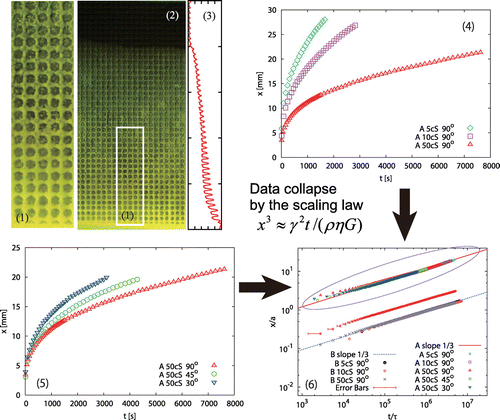
The imbibition dynamics is shown in Figure 3(4) and (5): the viscosity of the oil as well as gravity slows down the dynamics (to change ‘gravity,’ the substrate is tilted from the vertical position for which the angle is defined to be 90).

The data in Figure 3(4) and (5) show that both viscosity and gravity is important, whereas capillarity is the driving force, which leads to the following scaling argument to be confirmed by a clear data collapse. In the Navier–Stokes equation, the driving force corresponds to the pressure gradient term, which can be expressed as , with and the curvature and the imbibition height, respectively. The viscous term scales as with the viscosity of oil and is a viscous length scale. The gravity term is expressed as with and the density of oil and the effective gravitational acceleration, i.e. . The capillary-gravity balance, , fixes the radius of curvature as , which decreases with the imbibition height. As suggested in Figure 3(1)–(3) (see in particular, the brightness analysis in (3)), the film thins down with height, whereas the viscous length scale may be the thickness of the film. It is, thus, reasonable to identify the radius of curvature, which decreases with height, with the viscous length, i.e. . With this identification, the viscous-gravity balance, , results in the following scaling law:(6)

On the basis of this law, a distinct data collapse can be shown as in Figure 3(6). The curves in Figure 3(4) and (5) collapse convincingly onto a single master curve in Figure 3 (6).

Equation (6(6) ) stating that the imbibition length scales with is in contrast with the usual viscous regime of capillary rise or the imbibition dynamics observed on textured surfaces decorated with relatively high pillars with sharp head edges (see, e.g. [9,10]): in most cases, scales with . However, the same law has been observed in rather different context of capillary rise into corners [11–13]. It seems that there are many different scaling regimes for the imbibition of various types of texture surfaces, especially because the problems boil down essentially to the imbibition of open capillaries in which free liquid surface expands as the imbibition proceeds [13].

4. Granular drag friction for an obstacle in the Hele-Shaw cell

A naive question associated with the different scaling regimes shown for viscous drag friction in the Hele-Shaw cell would be how the friction law would be changed if fluids are replaced with granular particles in the cell. The set-up for answering this question is shown in Figure 4(a) and (b). The cell is mounted on the slider and the slider can move the cell at a constant speed. During the movement, the drag force acting on the obstacle can be monitored by the force gauge because the obstacle and the force gauge is connected by a non-extensible strong fishing line. Result for measured force vs. time at different packing fraction are given in Figure (c). The force fluctuates considerably with time, but an average at each can be well defined as indicated by the three horizontal lines. As the fraction increases, both the average and fluctuation of drag force increase.

Figure 4. (colour online) (a) and (b) Set-up for the experiment for granular drag friction. (a) View of the cell from above. (b) Slanted view of the set-up. One layer of granular particles of average diameter d = 2 mm are packed in a two-dimensional cell made of transparent acrylic plates. The diameter of the obstacle is about 10 times larger than . (c) Drag force vs. time . The force fluctuates in time significantly, but with a well-defined average. (d) The average drag force vs. the drag velocity for all packing fractions we investigated (the error bars that represent fluctuations are suppressed here for simplicity). Remarkably, is a smooth function of . The average force and fluctuation (not shown) both increase with the packing fraction . (e) Data collapse of the plot in (d) as a result of replotting the renormalized dynamic component of drag force as a function of the renormalized velocity , according to the theory (f) and (g): divergence of the dynamic (f) and static (g) components of the force at the jamming point . (h) Total force divided by the divergent factor vs. velocity . Plots are reproduced from [36].

The average force is found to be a smooth function of the drag velocity with force and fluctuation increased with the packing fraction , as demonstrated, in Figure 4(d), for all the packing fractions we studied. Here, the error bars, i.e. the fluctuations are removed for clarity. In fact, all the curves are well described in the form with both and dependent on .

The dynamic component of the drag force can be explained as follows. This component may be estimated as the momentum transfer per time. The momentum transfer occurs when the obstacle collides with a small particle. The frequency can be estimated as with and are the radius of the disk obstacle and is the average diameter of slightly polydispersed grains (the thickness of the obstacle is also and that of cell is slightly larger than ). If collisions were a two- body collision, the momentum transfer per collision should scale as with the mass of grains. However, as the packing fraction increases, grains ahead of the obstacle should be somewhat jammed [14] or shear jammed [15]. As a result, the obstacle collides with a cluster of grains each time it collides with a single grain. Naturally, the characteristic cluster size increases with the packing fraction , suggesting the observed increase in the average force with . To estimate the cluster size , we consider empty space around the obstacle below the jamming point at . In the region around the obstacle of area , the empty area scales as . The cluster size may be determined in such a way that this area scales with the obstacle area, i.e. , which means that this length scale diverges towards the jamming point. The cluster area is now estimated as : we expect the length scale in the velocity direction obtained above is separated from the length in the direction perpendicular to it because of shear in the moving direction acting in the granular medium. The cluster tends to be broken in the perpendicular direction. This assumption means that the momentum transfer per each collision with a grain should scale as with the density of grains. Combined with the above expression for the frequency, , we obtain the relation,(7)

Note that the factors appearing in the frequency and in the momentum transfer can be replaced both with near the jamming point, and, thus, the two factors can be integrated into the numerical coefficient for the above scaling law. When we rescale the dynamic component and velocity in Figure 4(d) according to the above scaling law, in the form, with(8)

we obtain a remarkable data collapse as shown in Figure 4(e). The exponent of the divergence is confirmed in Figure 4(f).

The static component also scales with : this force is also divergent towards the jamming point. This is justified theoretically and experimentally as follows. When collisions become negligible as velocity decreases, drag friction tends to be dominated by friction with the bottom wall. When the cluster area is much larger than the disk size, as in the region near the jamming point, the friction force can be estimated as , with the friction coefficient:(9)

This divergence is well confirmed in Figure 4(g). When Equation (9(9) ) is combined with Equation (7(7) ), it follows that the total force should scale with the divergent factor , which can be directly confirmed in Figure 4(h) (all the data shown here are obtained for the same and ). In addition, the order of magnitude of predicted by Equation (9(9) ) is consistent with the experimental data: Figure 4(h) shows that is of the order of 0.1 N. This is exactly the order of magnitude of , which scales as according to Equation (9(9) ): for , kg/m, m/s, mm, we obtain N.

The crossover between slow and velocity regimes can be well defined by comparing the right-hand side of Equation (7(7) ) and that of Equation (9(9) ): the ratio of the former to the latter is expressed as with(10)

This crossover velocity is in fact another expression of given in Equation (8(8) ), i.e. , because the divergent factors in and are cancelled out in Equation (8(8) ). The orders of magnitude of the right-hand side of Equation (10(10) ), , is estimated as 10 mm/s, which compares well with 100 mm/s, above which the law is established as in Figure 4(e).

Some comments are as follows. (1) In [16], the dependence of Equation (7(7) ) on the disk radius is established through the agreement between theory and experiment. (2) It seems that Equations (7(7) ) and () break down in a low-velocity region : the above scaling regimes are in a rather high-velocity regime. In the present set-up, however, it is technically more difficult to explore in a low-velocity region: with velocity decreases the drag friction force decreases and in such a case the friction with the bottom and top covers of the cell becomes non-negligible; we have to establish a way to remove this component. As for low-velocity regions, there have been many related studies (e.g. [17–25]), while the high-velocity region studied here may be compared with impact experiments [26–28], in which, however, the packing fraction cannot be controlled. (3) Visualization of the diverging length scale has yet to be explored. (4) The results discussed above are essentially reproduced in numerical simulation [29]. (5) The growth of the fluctuations, apparent from Figure 4(c), has been also analysed [16]: it diverges again as . The statistics of the fluctuations seems to be a Gaussian type, in contrast with a recent study [26].

Figure 5. (colour online) (a) Remarkable micro-structure found in nature. Magnified images of the sections of nacre (left; courtesy of Prof. Dinesh Katti) and the exoskeleton of lobster (right; taken from [37]). (b) Illustration of a simplified model of nacre with a crack and structure parameters in the model at the scale of layer structure (left) and the scale of sample size (right). Created from [30]. (c) Stress distribution under the presence of a line crack in a plate of nacre (left) and a monolith of the hard element of nacre (right) with an intensity scale (middle), obtained by finite element calculations. Stress concentration near the crack tips is significantly reduced in nacre. (d) Crack shape near the tip (left) and collapse of the data (right), confirming the scaling law shown in the panel. The plots show that the deformation is more enhanced for smaller (the case corresponds to real nacre). (c) and (d) Created from data in Ref. [32]

5. Strength of biological materials

In nature, there are a number of strong and tough materials exploiting a magnificent micro-structures, as shown in Figure 5(a). The layered structure of nacre, found inside certain seashells like abalone and on the surface of pearl, is one of the most well-studied examples as such (see Figure 5(a) left). In the case of the exoskeleton of lobster, similar layer structures with different two periods can be observed as shown in Figure 5(a) right (in fact, these layer structures originate from magnificent substructures). In the following, we focus on the nacre structure, although a simple model for nacre introduced below can be applied also for the structure of the exoskeleton of lobster [30].

The layered structure of nacre is viewed as composed of hard layers (of micron-scale thickness ) and soft layers (of nanoscale thickness ). This thickness contrast implies that the soft component is very minor. The hard component is aragonite, a crystalline form of CaCO, while the soft component is mainly composed of proteins. Because the latter volume content is small, we can see only plates of aragonite in Figure 5(a) left. However, as we will see below, a small amount of soft component drastically changes the mechanical response. The hard and soft elastic moduli are denoted and , respectively, and we introduce a small parameter , which is defined as .

From the simple elastic model of the layered structure, we can predict the stress field near the tips of a line crack of length in a two-dimensional plate of height and of width (), together with the deformation field , with () the distance from a crack tip (see Figure 5(b)). As shown in the left illustration in Figure 5(b), we consider a simple layered structure with the above introduced parameters , , , , and . Typical values of these parameters are shown in the right illustration in Figure 5(b). We introduce a line crack perpendicular to the layered structure as suggested in both of the illustrations in Figure 5(b). The sample is then stretched in the direction (the direction parallel to the layers) under a fixed griped condition (namely, deformations and (both independent of ) are respectively applied at the top and end bottom edges of the sample). When we consider this problem in the limit of small , we can show that the dominant components of stress and strain in the corresponding equilibrium state are the and components, and , respectively, because of the anisotropic nature of the problem. In addition, we can show the equilibrium deformation field is governed by an anisotropic two-dimensional Laplace equation on the plane,(11)

with ( is the Poisson’s ratio), subject to the corresponding boundary conditions. In fact, we can obtain full analytical solutions for the fields by the conformal mapping augmented by a special transformation that allows us to remove singularity appearing at the surfaces of the crack. From the analytical solutions when the crack size is much larger than the plate height (see below for the details), we can derive the following scaling laws that are valid near the tip [31]:(12) (13)

Here, and are the stress and deformation away from the crack tip.

The scaling laws suggest that stress concentration near the tip is weakened by the small factor whereas the deformation is enhanced by the large factor . The former statement supports the strength of nacre: a material fails mainly due to the enhanced stress near tips of cracks, which is restricted here by the small factor (This is demonstrated in the results of finite element calculations shown in Figure 5(c)). The latter statement suggests the physical reason for the reduction of the tip stress concentration. As seen in Figure 5(d) left, as the soft modulus (i.e. ) becomes smaller, the deformation in soft layers is increased, which in turn reduces the deformation in hard layers. A weak deformation in hard layer should lead to a weak stress concentration, because this material is predominantly composed by the hard element.

The robustness of the scaling laws is demonstrated by finite element calculations based on the same layered model performed by the software, ABAQUAS [32]. The data collapse of the calculation data by the above scaling law for is shown in Figure (d), namely, the curves for the deformation field as a function of the distance from the tip presented in the left for different are well collapsed in the right by rescaling of both axes following Equation (13(13) ). In fact, the numerical calculations are involved with a number of length scales that should be well separated with each other: the set of conditions should be well satisfied for the approximations leading to Equations (12(12) ) and (13(13) ) are valid. However, some of the conditions are only marginally satisfied. Nonetheless, the data collapse in Figure 5(d) right is clear (a similar collapse is confirmed also for ), suggesting the robustness of the scaling laws.

We explain the robustness of scaling law in a more specific manner. The approximate expression in Equation (13(13) ) is obtained via the following expression [33]:

where and as before. In the limit , this expression certainly reduces to Equation (13(13) ): we may tend to say this expression is valid for However, it would be more precise to say this expression is valid for , and this condition is satisfied even if : even for , the size of the correction is considerably smaller than unity. In fact, the collapsed data in Figure 5(d) right includes the case when : even though the condition is only marginally satisfied, the scaling law is valid. This is an example in which a scaling law appears ‘robust.’

A few other scenarios for an apparently robust scaling law are as follows. When a scaling law is obtained as a result of series expansion, , we may tend to say that this scaling law is valid when . However, this law is in fact well satisfied even when , for the sake of a small pre-factor . When the same scaling law is instead obtained from the series, , in which the leading correction term starts from the third-order term, the scaling law can be well satisfied even when is not well satisfied; e.g. for , we have a fairly small correction, . In many experiments and when constructing a scaling phenomenology, we do not know the exact analytical mechanism leading to a scaling law in advance. However, the above scenarios guaranteeing a possibility for a scaling law to be ‘robust’ may encourage experiment and phenomenology seeking scaling laws (although we can think of other scenarios unfavourable for scaling laws).

Finally, we note that the fracture toughness can be also estimated [31] and the orders of magnitude is comparable to experimental measurements [34]. Further details including the background for tough biological materials can be found in a recent review [30].

6. Discussion

We have seen that scaling arguments are a powerful tool to unveil the physical mechanism of the problem in question, and this approach is universally useful for a variety of problems in the following respects. (1) The approach can extract the physical essence of the problem. Scaling laws are usually obtained through balances of energies or forces of various physical origins, and, thus, provide simple views and ‘intuitions’ on the problem. (2) Scaling laws obtained in the course might be simple enough to be useful as a guiding principle to develop products or to control the product quality. In such a case, scaling laws could make a strong impact on various applications, including those in industry. (3) A scaling law can be robust in the sense that it can be nearly exact even if the limiting condition for the law to be valid is only marginally satisfied or even weakly violated. This makes the scaling approach useful in a wide range of situations. (4) The validity of scaling laws can be made often through a distinct data collapse, which is a rather subjective way to establish the agreement between theory and experiment. (5) A clear data collapse determines the numerical coefficient for the scaling law, giving a prediction for future detailed studies and impacting on the field of research. The most serious weakness of the scaling analysis is that we cannot determine a dimensional numerical coefficient, but this weak point can be overcome via fitting onto experimental data. This implies the importance of a good coordination of experimental and theoretical studies. (6) The approach is especially useful for problems of complex phenomena in daily life or those related in industrial applications, with which physicists have hesitated to tackle because of the difficulty coming from the complexity. However, it is useful also for any new problems in physics to make a first step that is sound.

In conclusion, the scaling approach is a powerful method for pioneers in any fields of physical science. The author hopes that this short note will inspire such pioneers to curve out new frontiers of physical sciences.

Acknowledgements

The author is most grateful to the late Pierre-Gilles de Gennes, Françoise Brochard and David Quéré for what the author has been given through discussions, articles and textbooks such as [4,5,35]. The author thanks Hisao Hayakawa and Satoshi Takada (both, Kyoto University) for discussions on granular drag friction.

Additional information

Funding

This work was partly supported by Grant-in-Aid for Scientific Research (A) No. [24244066] of JSPS, Japan, and by ImPACT Program of Council for Science, Technology and Innovation (Cabinet Office, Government of Japan).

Notes

No potential conflict of interest was reported by the author.

References

- T. Lee , Particle Physics and Introduction to Field Theory , Harwood Academic Press, Newark, NJ, 1981.
- T. Anderson , Fracture Mechanics , 2nd ed., CRC Press, Boca Raton, FL, 1995.
- J. Cardy , Scaling and Renormalization in Statistical Physics , Vol. 5, Cambridge University Press, Cambridge, 1996.
- P.G. De Gennes , Scaling Concepts in Polymer Physics , Cornell University Press, Ithaca, NY, 1979.
- P.G. de Gennes , F. Brochard-Wyart and D. Quéré , Gouttes, Bulles, Perles et Ondes , 2nd ed., Berlin, Paris, 2005.
- A. Eri and K. Okumura , Soft Matter 7 (2011) p.5648.
- M. Yokota and K. Okumura , Proc. Nat. Acad. Sci. (USA) 108 (2011) p.6395.
- A. Eri and K. Okumura , Phys. Rev. E 82 (2010) p.030601(R).
- C. Ishino , K. Okumura and D. Quere , Europhys. Lett. 68 (2004) p.419.
- M. Tani , D. Ishii , S. Ito , T. Hariyama , M. Shimomura and K. Okumura , Plos One 9 (2014) p.e96813.
- L.-H. Tang and Y. Tang , J. Phys. II Fr. 4 (1994) p.881.
- A. Ponomarenko , D. Quéré and C. Clanet , J. Fluid Mech. 666 (2011) p.146.
- M. Tani , R. Kawano , K. Kamiya and K. Okumura , Sci. Rep. 5 (2015) p.10263.
- A.J. Liu and S.R. Nagel , Nature 396 (1998) p.21.
- D. Bi , J. Zhang , B. Chakraborty and R. Behringer , Nature 480 (2011) p.355.
- Y. Takehara , S. Fujimoto and K. Okumura , EPL (Europhys. Lett.). 92 (2010) p. 44003.
- K. Wieghardt , Annu. Rev. Fluid. Mech. 7 (1975) p.89.
- R. Albert , M. Pfeifer , A.L. Barabási and P. Schiffer , Phys. Rev. Lett. 82 (1999) p.205.
- R.R. Hartley and R.P. Behringer , Nature 421 (2003) p.928.
- D. Chehata , R. Zenit and C.R. Wassgren , Phys. Fluids 15 (2003) p.1622.
- M.B. Hastings and C.J. Olson , Reichhardt and C. Reichhardt: Phys. Rev. Lett. 90 (2003) p.098302.
- J.A. Drocco , M.B. Hastings , C.J.O. Reichhardt and C. Reichhardt , Phys. Rev. Lett. 95 (2005) p.088001.
- D.J. Costantino , T.J. Scheidemantel , M.B. Stone , C. Conger , K. Klein , M. Lohr , Z. Modig and P. Schiffer , Phys. Rev. Lett. 101 (2008) p.108001.
- R. Candelier and O. Dauchot , Phys. Rev. Lett. 103 (2009) p.128001.
- E. Kolb , P. Cixous , N. Gaudouen and T. Darnige , Phys. Rev. E 87 (2013) p.032207.
- A.H. Clark , L. Kondic and R.P. Behringer , Phys. Rev. Lett. 109 (2012) p.238302.
- D.I. Goldman and P. Umbanhowar , Phys. Rev. E 77 (2008) p.021308.
- H. Katsuragi and D.J. Durian , Nat. Phys. 3 (2007) p.420.
- S. Takada and H. Hayakawa (2015), arXiv preprint arXiv:1504.04805.
- K. Okumura , MRS Bull. 40 (2015) p.333.
- K. Okumura and P.G. de Gennes , Eur. Phys. J. E 4 (2001) p.121.
- Y. Hamamoto and K. Okumura , Adv. Eng. Mater. 15 (2013) p.522.
- Y. Hamamoto and K. Okumura , Phys. Rev. E 78 (2008) p.026118.
- A. Jackson , J. Vincent and R. Turner , Proc. R. Soc. (London) B. 234 (1988) p. 415.
- P.G. de Gennes , Soft Interfaces: The 1994 Dirac Memorial Lecture , Cambridge University Press, Cambridge, 2005.
- Y. Takehara and K. Okumura , Phys. Rev. Lett. 112 (2014) p.148001.
- H. Fabritius , C. Sachs , P. Triguero and D. Raabe , Adv. Mater. 21 (2009) p.391.