Vacancy encounter model for stochastically fluctuating electric field gradients in the Cu₃Au crystal structure

ABSTRACT

A class of experimental techniques known as hyperfine methods can be used to measure electric field gradients (EFGs) through the hyperfine interaction experienced by tracer nuclei. When EFGs fluctuate at rates comparable to the inverse characteristic timescale of the hyperfine method, there is a loss of signal coherence that can be used to determine EFG fluctuation rates. This has been used to measure, for example, EFG fluctuations accompanying atomic jumps of radiotracers using perturbed angular correlation spectroscopy (PAC). Nominally, there is a one-to-one correspondence between EFG fluctuation and tracer jump, but when tracer jumps are mediated by a vacancy diffusion mechanism, a subset of multiple tracer-vacancy exchanges will not affect spectra when they occur much faster than the hyperfine timescale, leading to an underestimate of underlying tracer jump rate if this correlated random-walk effect is not taken into consideration. The present work calculates the factor by which EFG fluctuation rate differs from tracer jump rate based on a time-dependent, random-walk analysis of tracer displacement probabilities in a vacancy encounter model for the special case of self-diffusion in the L1₂ crystal structure.

KEYWORDS:

• Diffusion
• defect concentration
• encounter model
• atomic displacement probability

Introduction

Conventionally, atomic motion in solids is studied by monitoring the evolution of concentration profiles of radioactive tracer atoms [1,2]. Alternatively, one can use an experimental method that is sensitive to an observable that changes as a result of an atomic jump. One such observable is the electric field gradient (EFG) present at the nucleus of a diffusing atom. It can be measured via the electric quadrupole interaction using a number of different techniques known collectively as hyperfine methods including Mössbauer spectroscopy, nuclear magnetic resonance (NMR), and perturbed angular correlation spectroscopy (PAC) [3].

The EFG is a traceless, second-rank tensor that is essentially the second spatial derivative of the electrostatic potential. The symmetry of the EFG experienced by a nuclear tracer, therefore, is the same as the point symmetry at the lattice site the tracer occupies. Depending on the crystal structure, tracers may be distributed among lattice sites that are crystallographically equivalent but experience EFGs that are orientationally inequivalent. The hyperfine methods are sensitive to orientational changes in EFGs that occur, for example, as the radiotracers jump among sites.

Spectra of hyperfine methods are obtained from ensembles of nuclei. Random fluctuations in EFGs experienced by these nuclei can result in a decoherence in signal, leading to a damping in spectra collected in the time domain or broadening in the frequency domain. Such effects will only be observable when the fluctuations occur on the same timescale as the hyperfine method [4]. For example, the timescale of a PAC measurement is determined by the lifetime of the intermediate nuclear level of the radiotracer, which is 121 ns for the most commonly used ¹¹¹In isotope. The time resolution of a typical experimental apparatus allows measurement of degrees of damping accompanying fluctuation rates that are factors of roughly 10⁻²–10⁺³ of the inverse intermediate state lifetime, or about 80 kHz to 8 GHz for ¹¹¹In. For fluctuations that occur at higher rates, caused, for example, by random atomic motion due to lattice vibrations, damping of PAC signals is not observed with measured EFGs determined by time-averaged positions of atoms near the radiotracers.

A point defect such as a vacancy near the radiotracer breaks the local point symmetry and changes the EFG experienced by the radiotracer, and random jumps of the defect will lead to EFG fluctuations that can be measured using PAC if the jumps occur at the same timescale of the method. The rate at which a vacancy exchanges with an atom in a neighbouring position can be expressed as $\nu \exp \left(-\mathrm{\Delta }{H}_{\mathrm{m}}/k_{\mathrm{B}}T\right)$ where $\mathrm{\Delta }{H}_m$ is the migration enthalpy barrier and $\nu$ is the jump attempt frequency. Because $\mathrm{\Delta }{H}_m>0$, the vacancy jump rate increases as temperature increases, and often there will be a temperature range for which the vacancy jump rate falls within the 80 kHz to 8 GHz for ¹¹¹In.

A universal approach for calculating lineshapes in the presence of time varying hyperfine interactions was put forth by Dattagupta [5]. The stochastic EFG fluctuation model considered in this work has been called variously a jump process [5], a Kubo-Anderson process (KAP) [6,7], the strong collision approximation [8], and the random phase approximation [9]. In this model, EFG changes occur within infinitesimal time interval dt with probability densities given by transition rates that are independent of history. Model parameters include EFG tensor components and average rates of transition, or fluctuation rates, among EFGs [10]. Nominally, there is a one-to-one correspondence between changes in EFG and atomic jumps. If the jumps produce EFG changes that are much faster or slower than the hyperfine timescale, however, the damping will be too small to observe.

The present work considers systems in which the radiotracers themselves exchange with neighbouring vacancies and there is a reorientation of the EFG accompanying the change in tracer lattice location. For simplicity, it considers the special case of negligible attractive interaction between the tracer and vacancy, as would be the case, for example, for self-diffusion, with small vacancy concentration. This means that at low temperature (i.e. for low vacancy jump rates) the number of tracers with vacancies within one or two first-neighbour shells immediately following radioactive decay would be too small to lead to a measurable fraction of tracers with EFGs disturbed by the local symmetry-reducing vacancies. At higher temperature, vacancy jumps will be more rapid so that vacancies can jump next to and exchange with tracers within the timescale of the hyperfine method. Because vacancies must make multiple jumps, on average, before reaching a site next to a tracer, the vacancy jump rate must be much faster than the inverse hyperfine timescale and EFGs disturbed by vacancies go undetected. This was verified, for example, in stochastic EFG simulations for the Cu₃Au crystal structure [11,12] for sufficiently small vacancy concentrations.

In this situation, EFG fluctuations can be related to atomic jump processes according to the following basic sequence of events described by the vacancy encounter model [13]: (1) a vacancy moves into a first neighbour position of the tracer, (2) the tracer and vacancy exchange, which demarks the start of the encounter, and (3) the vacancy continues to jump near the tracer so that the tracer and probe may re-exchange one or more times. Conventionally, the encounter is said to end when the tracer and vacancy make their final exchange. Because there is a possibility that the vacancy and tracer re-exchange one or more times following step (2), it is possible that the tracer winds up on a lattice site that has the same EFG as it had before the encounter, in which case the encounter would go undetected. As a result, the tracers jump at a higher rate than measured EFG fluctuation rate.

For simplicity, a high-symmetry crystal system for which all vacancy jumps have the same jump frequency is considered. The rate at which an EFG changes from one distinct state to another distinct state, r, will be related to the frequency at which vacancy encounters occur, w_e, by $r=w_e{P}_{\mathrm{\Delta }\mathrm{E}\mathrm{F}\mathrm{G}}$ where $P_{\mathrm{\Delta }\mathrm{E}\mathrm{F}\mathrm{G}}$ is the probability that the encounter leads to the change in EFG. The encounter rate w_e depends on vacancy concentration, c_v, and the rate at which a vacancy-tracer exchanges if a vacancy is next to the tracer, w₂, according to w_e = Zc_v w₂/N_e, where Z is the number of first neighbour jumps accessible to the tracer and N_e is the average number of tracer-vacancy exchanges per encounter [14]. All together, this gives(1) $r=P_{\mathrm{\Delta }\mathrm{E}\mathrm{F}\mathrm{G}}Z{c}_{\mathrm{V}}{w}_2/N_e.$(1)

The P_ΔEFG, can be calculated by summing the probabilities of a tracer displacement by l during an encounter, W(l), over the set of vectors l that lead to the selected change in EFG. The displacement probabilities and number of jumps per encounter depend on the duration of the encounter. For example, the longer the encounter the more vacancy-tracer exchanges can occur so that the W(l) corresponding to larger magnitude l become relatively larger. Baker et al. showed how to calculate these time-dependent quantities, N(t) and W(l,t) for self-diffusion in the simple-cubic lattice structure in the case of infinitesimal vacancy concentration [15]. Dasenbrock-Gammon and Zacate built on that work to show how to calculate time-averaged quantities $N_{\mathrm{e}}\left(c_{\mathrm{V}}\right)\equiv \int f\left(c_{\mathrm{V}},t\right)N\left(t\right)dt$ and $W\left(\mathbf{l},c_{\mathrm{V}}\right)\equiv \int f\left(c_{\mathrm{V}},t\right)W\left(\mathbf{l},t\right)dt$ as functions of finite vacancy concentration, which enters through the factor $f\left(c_{\mathrm{V}},t\right)$, the probability density that a second vacancy exchanges with the tracer at time t, thereby interrupting an encounter [16]. Note that because analysis of the EFG transition rates in the stochastic model is based on time-averaged rates, the P_ΔEFG and N_e factors needed in Equation 1 depend only on vacancy concentration and are independent of the underlying vacancy jump rate.

EFG fluctuation rates due to diffusion of radiotracers on the Cu sublattice of Cu₃Au-structured compounds have been studied extensively using PAC [17–21]. It is, therefore, desirable to adapt the theoretical methods described above to calculate quantities N_e and $P_{\mathrm{\Delta }\mathrm{E}\mathrm{F}\mathrm{G}}$ for diffusion via the vacancy mechanism on the Cu sublattice of the Cu₃Au structure in order to relate EFG fluctuation rates to tracer jump rates. The present work does this for the special case of self-diffusion.

Method

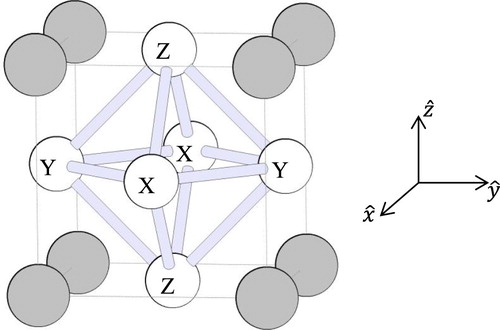
The Cu₃Au crystal structure is shown in Figure 1. The Cu sites are located at the vertices of a network of octahedrons. There is one crystallographically unique Cu site with 4/mmm site symmetry so that a tracer at a Cu site experiences an axially symmetric EFG with main principal component oriented parallel to the symmetry axis. There are three possible orientations for the symmetry axis, which means that despite there being a single crystallographically unique site, there are three EFG-orientationally inequivalent Cu sites. These ‘site types’ will be referred to as X, Y, and Z for symmetry axis along the x, y, and z Cartesian directions, respectively.

Figure 1. The Cu₃Au crystal structure. Au sites are shaded and Cu sites are labelled according to the Cartesian direction in which the principal EFG component with largest magnitude is oriented. First-neighbour Cu sites within the unit cell are connected by lightly shaded bars. For each site, only half the first neighbour connections are shown, the other connections extend into neighbouring unit cells.

In this work, motion of vacancies on the Cu sublattice is considered. The vacancies are assumed to undergo a random walk with mean residence time τ between jumps. In this case, the probability that a vacancy has jumped k times within time t, $w_k\left(t\right)$, is given by the Poisson distribution [15]:(2) $w_k\left(t\right)=\frac{1}{k!}{\left(\frac{t}{\tau }\right)}^k\exp \left(-t/\tau \right).$(2) The rate at which a vacancy jumps in a single direction is equal to $(Z\tau {)}^{-1}$. That is, $dt(Z\tau {)}^{-1}$ is the probability that the vacancy jumps in a single direction within the time interval dt. For the case of self-diffusion, the tracer-vacancy exchange rate, w₂ in Equation 1, is equal to $(Z\tau {)}^{-1}$.

Each site type has Z = 8 first neighbours, four of one site type and four of another. One can define 8 sets of displacement vectors by ${\mathbf{d}}_i^{\alpha \to \beta }$, which denotes the i^th of 4 possible jumps from a site of type α to a site of type β, where $\beta \ne \alpha$ in this crystal structure. Throughout this work, lower-case Greek letters (except for φ) are used to denote a variable site type; that is, for example, $\alpha \in \left\{X,Y,Z\right\}$. Furthermore, the arrow in the superscript indicates the direction a vacancy moves, so that if a vacancy displacement results in a tracer-vacancy exchange, then the tracer is displaced by $-{\mathbf{d}}_i^{\alpha \to \beta }$.

Two different paths of a vacancy undergoing a random walk that result in at least one exchange with a tracer atom initially located on a site type Z are considered in Figure 2. When the vacancy is far away from the tracer, the tracer experiences an axially symmetric EFG with main principal component oriented along the z direction. In path 1, the sequence of jumps takes the vacancy to a site type Y in a first neighbour position of the tracer (frame 1c). The next vacancy jump results in an exchange with the tracer, after which the tracer experiences a new non-axially symmetric EFG (frame 1d). The vacancy next jumps away from the tracer, which then experiences an axially symmetric EFG along the y direction. In path 2, the vacancy undergoes a different sequence of jumps after the initial exchange with the tracer (between frames 2c and 2d) so that it exchanges with the tracer a second time (between frames 2 g and 2 h) before it moves away. There are two basic outcomes of a vacancy randomly exchanging with a tracer: a reorientation of the main principal axis of the axially symmetric EFG by 90° as in path 1, or no change in the EFG as in path 2.

Figure 2. Snapshots showing positions of a vacancy on the Cu sublattice as it jumps along two different paths near a tracer in the Cu₃Au crystal structure. Each frame (labelled a–j) shows the system after successive vacancy jumps so that one frame increment corresponds to one vacancy jump and the system remains in the configuration shown in each frame for an average duration equal to the mean residence time of the vacancy, τ. In each configuration, the EFG experienced by the tracer is represented by three line segments representing the EFG principal axes. Au is represented by large spheres, Cu is represented by small spheres, and the tracer is indicated by a radioactivity symbol.

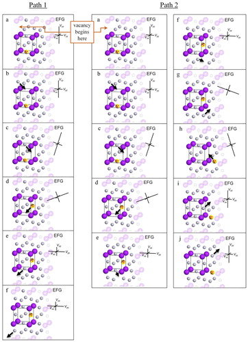
As is shown in Figure 2, when the vacancy is near the tracer, it disturbs the EFG so that the tracer experiences a transient, non-axially symmetric EFG (frames 1c, 1d, 2c, 2d, 2g, and 2h). This work considers vacancy concentrations small enough that the mean residence time of the vacancy in any given position, τ, is orders of magnitude smaller than the time between encounters, 1/w_e. Thus, when the time between encounters is on the same timescale as the hyperfine method, τ is too small for the non-axial EFG fluctuations to affect the spectrum. That is, impacts of non-axial EFGs can be neglected for low vacancy concentration so that to an excellent approximation, the tracers experience stochastic fluctuations of axially symmetric EFGs among three orthogonal directions, which is well-studied and known as the XYZ model [22–25].

The XYZ-model parameter of interest in the present work is the EFG reorientation rate, represented by r in Equation 1. Simulations of PAC spectra for the ¹¹¹In isotope generated using the XYZ model are shown in Figure 3 for a range of reorientation rates. More details on the theory behind calculation of these lineshapes and example simulations for other hyperfine methods can be found in Ref. [5].

Figure 3. Simulations of PAC spectra G₂(t) for the ¹¹¹In isotope and corresponding FFTs G₂(ω) for the XYZ model generated using the Stochastic Hyperfine Interactions Modeling Library [10,26]. The quadrupole interaction frequency ω_Q was taken to be π/(3τ₀) where τ₀ is the lifetime of the intermediate PAC level. At very low reorientation rate, r < τ₀, the spectrum is undamped/unbroadened (a). In the slow fluctuation regime, r << τ₀, the spectrum is damped/broadened by an amount propotional to r (b). In the rapid fluctuation regime, r > τ₀, the spectrum is damped/broadened by an amount inversely propotional to r and exhibits an observed frequency corresponding to the motionally averaged limit, which is zero for the XYZ model (c). At very high reorientation rates, r >> τ₀, the spectrum exhibits an undamped/unbroadend, motionally averaged signal (d).

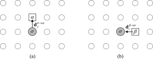
Because encounters such as shown in path 2 of Figure 2 do not result in a reorientation of EFG, calculations of N_e and P_ΔEFG via W(l) are needed so that w₂ can be determined from experimentally measured values of r. Calculation of these parameters requires following the motion of the tracer during an encounter. The tracer only jumps each time a vacancy exchanges with it. The encounter begins when a vacancy first exchanges with the tracer, and the state immediately following this first exchange is considered the initial condition of the encounter. The tracer is located at a site of type σ, and the vacancy is located at a site of type α. It is convenient to define the tracer’s position at this initial stage as the origin and to describe the starting position of the vacancy by the appropriate first neighbour position of the origin: ${\mathbf{d}}_j^{\sigma \to \alpha }$. The vacancy then continues its random walk.

In order for the vacancy to later re-exchange with the tracer, its random walk must take it into a site next to the tracer. With the tracer still at a site of type σ, each possible first neighbour site is given by the vector $-{\mathbf{d}}_i^{\beta \to \sigma }$ with the negative sign chosen to indicate that the next jump of the vacancy that leads to an exchange of the tracer is in the direction ${\mathbf{d}}_i^{\beta \to \sigma }$. Figure 4 shows a schematic of the conditions immediately after the start and immediately before re-exchange in the vacancy encounter model. The probability that the vacancy makes the re-exchange on the (k + 1)^th vacancy jump from the direction $-{\mathbf{d}}_i^{\beta \to \sigma }$ within the time interval between t and t + dt is denoted by $R_{k,ij}^{\beta \sigma \alpha }\left(t\right)dt$, where the superscript indicates the site types of the tracer and vacancy in the re-exchange and initial conditions.

Figure 4. Schematic of tracer and vacancy positions (a) immediately after the start of the encounter at t = 0 and (b) just before the first re-exchange between times t and t + dt. The tracer is denoted by the shaded circle, the vacancy is shown as a square, and Greek letters indicate site types.

The probability density for a vacancy to re-exchange with the tracer for the first time between t and t + dt from any direction after any number of jumps, $R\left(t\right)$, is given by summing over all possible numbers of jumps and final-jump directions:(3) $R\left(t\right)=\sum _{k=0}^{\mathrm{\infty }}\left\{\sum _i{R_{k,ij}^{\beta \sigma \alpha }\left(t\right)|}_{\beta \ne \sigma }+\sum _i{R_{k,ij}^{\gamma \sigma \alpha }\left(t\right)|}_{\gamma \ne \beta }\right\},$(3) the result of which will be independent of starting site type σ or starting tracer position ${\mathbf{d}}_j^{\sigma \to \alpha }$.

As laid out by Baker et al. [15], N(t) can be expressed conveniently by the recurrence relation(4) $N\left(t\right)=1+{\int }_0^{t}R\left(t^{\mathrm{\prime }}\right)N\left(t-t^{\mathrm{\prime }}\right)d{t}^{\mathrm{\prime }}.$(4) A closely related quantity is the probability that the vacancy returns to the tracer from any direction within time t, p(t). It is given by$p\left(t\right)={\int }_0^{t}R\left(t^{\mathrm{\prime }}\right)d{t}^{\mathrm{\prime }}.$

In this crystal structure, the possible destination vectors and corresponding atomic jump probabilities depend on the site type of the tracer at the start. Here, $W_{}^{\sigma \to \gamma }\left(\mathbf{l},t\right)$ will denote the probability that a tracer is displaced from a site of type σ by vector l that takes it to a site of type γ within time t. This can be calculated by considering all possible pathways and times that take the tracer into the destination:(5) $W^{\sigma \to \gamma }\left(\mathbf{l},t\right)=\sum _{n=1}^{\mathrm{\infty }}{\int }_0^t\sum _{\beta \ne \gamma ,i}{W}_n^{\sigma ,\beta \to \gamma }\left(\mathbf{l},{\mathbf{d}}_i^{\beta \to \gamma },t^{\mathrm{\prime }}\right)\left[1-p\left(t-t^{\mathrm{\prime }}\right)\right]d{t}^{\mathrm{\prime }},$(5) where $W_n^{\sigma ,\beta \to \gamma }\left(\mathbf{l},{\mathbf{d}}_i^{\beta \to \gamma },t^{\mathrm{\prime }}\right)dt$ denotes the probability that the tracer started the encounter at a site of type σ and jumps to a site of type γ from a site of type β on the tracer’s nth jump, which occurs between t’ and t’ + dt’, along the jump vector $-{\mathbf{d}}_i^{\beta \to \gamma }$. The factor $\left[1-p\left(t-t^{\mathrm{\prime }}\right)\right]$ assures that no further re-exchange occurs between t’ + dt’ and t. The sum is over lattice site types β neighbouring the final destination site type γ, and j is the summation index over the different possible jumps from β to γ. The sum over n and integral over t’ account for all possible numbers of jumps and the full range of possible times for the tracer to reach the destination at l.

To this point, it has been assumed that the encounter finishes before a second vacancy exchanges with the tracer, an assumption that is exactly correct for an infinitesimal vacancy concentration. Finite vacancy concentration c_v can be considered by introducing the factor $f\left(c_{\mathrm{V}},t\right)$, which gives the probability that an encounter is interrupted between time t and t + dt when a second vacancy exchanges with the tracer. Assuming that vacancies are distributed randomly in the solid so that new vacancy encounters occur at a constant rate c_V /τ, the interruption probability is given by(6) $f\left(c_{\mathrm{V}},t\right)=\frac{c_{\mathrm{V}}}{\tau }\exp \left(-c_{\mathrm{V}}t/\tau \right).$(6) The time-averaged quantities are then expressed(7) $N_{\mathrm{e}}\left(c_{\mathrm{V}}\right)\equiv \int \frac{c_{\mathrm{V}}}{\tau }\exp \left(-c_{\mathrm{V}}t/\tau \right)N\left(t\right)dt$(7) and(8) $W_{}^{\sigma \to \gamma }\left(\mathbf{l},c_{\mathrm{V}}\right)\equiv \int \frac{c_{\mathrm{V}}}{\tau }\exp \left(-c_{\mathrm{V}}t/\tau \right)W_{}^{\sigma \to \gamma }\left(\mathbf{l},t\right)dt.$(8) The quantity c_v/τ is conveniently replaced by the symbol s so that the above equations more obviously represent Laplace transforms. That is,(9) $N_{\mathrm{e}}\left(c_{\mathrm{V}}\right)=sN\left(s\right)$(9) and(10) $W^{\sigma \to \gamma }\left(\mathbf{l},c_{\mathrm{V}}\right)=s{W}^{\sigma \to \gamma }\left(\mathbf{l},s\right).$(10)

The $N\left(s\right)$ is found through the Laplace transform of Equation 4, which gives(11) $N\left(s\right)=\frac{1}{s\left(1-R\left(s\right)\right)}.$(11) The remaining steps needed to derive expressions for calculation of $R\left(s\right)$ and $W^{\sigma \to \gamma }\left(\mathbf{l},s\right)$ can be broken into two logical groups: terms associated with vacancy return probabilities and operations on atomic displacement probabilities.

Vacancy return probabilities

At low vacancy concentration, vacancy motion is described well as a random walk. The probability that the vacancy starts at position v ₁ at a site of type σ and is found at a position v of site type α after the vacancy’s k^th jump without any restriction on where the vacancy had been during those k jumps, $P_k^{\alpha ,\sigma }\left(\mathbf{v},{\mathbf{v}}_1\right)$, can be found using the recurrence relation(12a) $P_k^{\alpha ,\sigma }\left(\mathbf{v},{\mathbf{v}}_1\right)=\frac{1}{Z}\left\{\sum _i{P}_{k-1}^{\beta \ne \alpha ,\sigma }\left(\mathbf{v}-{\mathbf{d}}_i^{\beta \to \alpha },{\mathbf{v}}_1\right)+\sum _i{P}_{k-1}^{\gamma \ne \beta ,\sigma }\left(\mathbf{v}-{\mathbf{d}}_i^{\gamma \to \alpha },{\mathbf{v}}_1\right)\right\}$(12a) for k > 0, and(12b) $P_0^{\alpha ,\sigma }\left(\mathbf{v},{\mathbf{v}}_1\right)={\delta }_{\mathbf{v}{\mathbf{v}}_1}{\delta }_{\alpha \sigma }.$(12b) The probability that the vacancy is found at site v after k jumps having started at v ₁ within time t can be expressed simply by multiplying the spatial and temporal factors: $P_k^{\alpha ,\sigma }\left(\mathbf{v},{\mathbf{v}}_1,t\right)=P_k^{\alpha ,\sigma }\left(\mathbf{v},{\mathbf{v}}_1\right)w_k\left(t\right)$.

In order for a vacancy to re-exchange with the tracer, it must first move into a site next to the tracer without having previously exchanged with the tracer (except, of course, for the exchange that started the encounter). For a vacancy starting at position ${\mathbf{d}}_j^{\sigma \to \alpha }$, the probability that a vacancy is found at $-{\mathbf{d}}_i^{\beta \to \sigma }$ for the first time at the k^th step within time t without having revisited the tracer’s position at the origin 0 can be expressed as(13a) $Q_{k,ij}^{\beta \sigma \alpha }\left(t\right)=P_k^{\beta ,\alpha }\left(-{\mathbf{d}}_i^{\beta \to \sigma },{\mathbf{d}}_j^{\sigma \to \alpha },t\right)-P_k^{\beta ,\alpha ;\sigma }\left(-{\mathbf{d}}_i^{\beta \to \sigma },{\mathbf{d}}_j^{\sigma \to \alpha },t;\mathbf{0}\right);k>0$(13a) and(13b) $Q_{0,ij}^{\beta \sigma \alpha }\left(t\right)={\delta }_{-{\mathbf{d}}_i^{\beta \to \sigma },{\mathbf{d}}_j^{\sigma \to \alpha }}\delta \left(t\right).$(13b) Here $P_k^{\beta ,\alpha ;\sigma }\left(-{\mathbf{d}}_i^{\beta \to \sigma },{\mathbf{d}}_j^{\sigma \to \alpha },t;\mathbf{0}\right)$ denotes the probability that that a vacancy is found at ${\mathbf{d}}_j^{\sigma \to \alpha }$ for the first time at the k^th step within time t after having visited site 0 at least one time. The Laplace transform of Equation 13 can be expressed(14a) $Q_{k,ij}^{\beta \sigma \alpha }\left(s\right)=\left\{P_k^{\beta ,\alpha }\left(-{\mathbf{d}}_i^{\beta \to \sigma },{\mathbf{d}}_j^{\sigma \to \alpha }\right)-P_k^{\beta ,\alpha ;\sigma }\left(-{\mathbf{d}}_i^{\beta \to \sigma },{\mathbf{d}}_j^{\sigma \to \alpha };\mathbf{0}\right)\right\}\frac{\tau }{{\left(s\tau +1\right)}^{k+1}};k>0$(14a) and(14b) $Q_{0,ij}^{\beta \sigma \alpha }\left(s\right)={\delta }_{-{\mathbf{d}}_i^{\beta \to \sigma },{\mathbf{d}}_j^{\sigma \to \alpha }}.$(14b) It is useful to define the generating functions $P^{\beta ,\alpha }\left(\mathbf{v},{\mathbf{v}}_1:z\right)\equiv {\sum }_{k=0}^{\mathrm{\infty }}{z}^k{P}_k^{\beta ,\alpha }\left(\mathbf{v},{\mathbf{v}}_1\right)$ and $P^{\beta ,\alpha ;\sigma }\left(\mathbf{v},{\mathbf{v}}_1;\mathbf{u}:z\right)\equiv {\sum }_{k=0}^{\mathrm{\infty }}{z}^k{P}_k^{\beta ,\alpha ;\sigma }\left(\mathbf{v},{\mathbf{v}}_1;\mathbf{u}\right)$ so that(15) $\sum _{k=0}^{\mathrm{\infty }}{Q}_{k,ij}^{\beta \sigma \alpha }\left(s\right)=\frac{\tau }{\left(s\tau +1\right)}\left\{P_k^{\beta ,\alpha }\left(-{\mathbf{d}}_i^{\beta \to \sigma },{\mathbf{d}}_j^{\sigma \to \alpha }:z\right)-P_k^{\beta ,\alpha ;\sigma }\left(-{\mathbf{d}}_i^{\beta \to \sigma },{\mathbf{d}}_j^{\sigma \to \alpha };\mathbf{0}:z\right)\right\}$(15) where $z\equiv (s\tau +1{)}^{-1}$. This, in turn, can be written as(16) $\begin{array}{r}\sum _{k=0}^{\mathrm{\infty }}{Q}_{k,ij}^{\beta \sigma \alpha }\left(s\right)=\frac{\tau }{\left(s\tau +1\right)}\\ & \times \left\{P^{\beta ,\alpha }\left(-{\mathbf{d}}_i^{\beta \to \sigma },{\mathbf{d}}_j^{\sigma \to \alpha }:z\right)-\frac{P^{\beta ,\sigma }\left(-{\mathbf{d}}_i^{\beta \to \sigma },\mathbf{0}:z\right)P_{}^{\sigma ,\alpha }\left(\mathbf{0},{\mathbf{d}}_j^{\sigma \to \alpha }:z\right)}{P^{\sigma ,\sigma }\left(\mathbf{0},\mathbf{0}:z\right)}\right\}\end{array}$(16) as shown by Sholl [27].

With the vacancy in position $-{\mathbf{d}}_i^{\beta \to \sigma }$, the probability that it then exchanges with the tracer in the time interval between t and t + dt can be written$R_{k,ij}^{\beta \sigma \alpha }\left(t\right)dt=Q_{k,ij}^{\beta \sigma \alpha }\left(t\right)\frac{dt}{Z\tau }.$The Laplace transform of Equation 3 can be written(17) $R\left(s\right)=\frac{1}{Z\tau }\sum _i\left\{\sum _{k=0}^{\mathrm{\infty }}{Q_{k,ij}^{\beta \sigma \alpha }\left(s\right)|}_{\beta \ne \sigma }+\sum _{k=0}^{\mathrm{\infty }}{Q_{k,ij}^{\gamma \sigma \alpha }\left(s\right)|}_{\gamma \ne \beta }\right\}$(17) with the ${\sum }_{k=0}^{\mathrm{\infty }}{Q}_{k,ij}^{\beta \sigma \alpha }\left(s\right)$ terms given by Equation 16. Calculation of $R\left(s\right)$, therefore, ultimately comes down to calculation of the generating functions $P_{}^{\beta ,\alpha }\left(\mathbf{v},{\mathbf{v}}_1:z\right)$.

The first step in obtaining a useful expression for calculating $P_{}^{\beta ,\alpha }\left(\mathbf{v},{\mathbf{v}}_1:z\right)$ is to take the Fourier transform of Equation 12 to obtain(18a) $\begin{array}{rl}{P}_k^{\beta ,\alpha }\left(\phi ,{\mathbf{v}}_1\right)& =\frac{1}{Z}\left\{P_{k-1}^{\gamma \ne \beta ,\alpha }\right(\phi ,{\mathbf{v}}_1)\sum _i\exp \left(-i\phi \cdot {\mathbf{d}}_i^{\gamma \to \beta }\right)\\ & +P_{k-1}^{\chi \ne \gamma ,\alpha }\left(\phi ,{\mathbf{v}}_1\right)\sum _i\exp \left(-i\phi \cdot {\mathbf{d}}_i^{\chi \to \beta }\right)\};k>0\end{array}$(18a) and(18b) $P_0^{\beta ,\alpha }\left(\phi ,{\mathbf{v}}_1\right)=\exp \left(-i\phi \cdot {\mathbf{v}}_1\right){\delta }_{\alpha \beta }.$(18b) It is convenient to define(19) ${\mathbf{P}}_k^{\sigma }\left(\phi ,{\mathbf{v}}_1\right)\equiv \left(\begin{array}{c}{P}_k^{X,\sigma }\left(\phi ,{\mathbf{v}}_1\right)\\ P_k^{Y,\sigma }\left(\phi ,{\mathbf{v}}_1\right)\\ P_k^{Z,\sigma }\left(\phi ,{\mathbf{v}}_1\right)\end{array}\right)$(19) and(20) $\mathbf{M}\left(\phi \right)\equiv \left(\begin{array}{ccc}0& \sum _i\exp \left(-i\phi \cdot {\mathbf{d}}_i^{Y\to X}\right)& \sum _i\exp \left(-i\phi \cdot {\mathbf{d}}_i^{Z\to X}\right)\\ \sum _i\exp \left(-i\phi \cdot {\mathbf{d}}_i^{X\to Y}\right)& 0& \sum _i\exp \left(-i\phi \cdot {\mathbf{d}}_i^{Z\to Y}\right)\\ \sum _i\exp \left(-i\phi \cdot {\mathbf{d}}_i^{X\to Z}\right)& \sum _i\exp \left(-i\phi \cdot {\mathbf{d}}_i^{Y\to Z}\right)& 0\end{array}\right).$(20) Then Equation 18 becomes ${\mathbf{P}}_k^{\sigma }\left(\phi ,{\mathbf{v}}_1\right)=\mathbf{M}\left(\phi \right){\mathbf{P}}_{k-1}^{\sigma }\left(\phi ,{\mathbf{v}}_1\right)$, or(21) ${\mathbf{P}}_k^{\sigma }\left(\phi ,{\mathbf{v}}_1\right)={\mathbf{M}}^k\left(\phi \right){\mathbf{P}}_0^{\sigma }\left(\phi ,{\mathbf{v}}_1\right).$(21) This leads to the expression(22) ${\mathbf{P}}_{}^{\sigma }\left(\phi ,{\mathbf{v}}_1:z\right)=\sum _{k=0}^{\mathrm{\infty }}{z}^k{\mathbf{P}}_k^{\sigma }\left(\phi ,{\mathbf{v}}_1\right)=\left(\mathbf{I}-z\mathbf{M}\left(\phi \right){)}^{-1}{\mathbf{P}}_0^{\sigma }\right(\phi ,{\mathbf{v}}_1).$(22)

The quantities N_e and $P_{\mathrm{\Delta }\mathrm{E}\mathrm{F}\mathrm{G}}$ will be independent of a tracer’s starting position, so it is sufficient to consider the single starting condition, σ = X, for example. In this case,(23) ${\mathbf{P}}_k^{\mathrm{X}}\left(\phi ,{\mathbf{v}}_1\right)=\left(\begin{array}{c}\exp \left(-i\phi \cdot {\mathbf{v}}_1\right)\\ 0\\ 0\end{array}\right),$(23) and Equation 22 can be expressed(24) $\begin{array}{rl}{\mathbf{P}}^{\mathrm{X}}\left(\phi ,{\mathbf{v}}_1:z\right)=& \sum _{k=0}^{\mathrm{\infty }}{z}^k{\mathbf{P}}_k^{\mathrm{X}}\left(\phi ,{\mathbf{v}}_1\right)=\frac{\exp \left(-i\phi \cdot {\mathbf{v}}_1\right)}{D\left(\phi \right)}\times \\ & \left(\begin{array}{c}1-\frac{1}{4}{z}^2{\cos }^2\left(a{\phi }_y/2\right){\cos }^2\left(a{\phi }_z/2\right)\\ \frac{1}{8}z\cos \left(a{\phi }_x/2\right)\cos \left(a{\phi }_y/2\right)\left[4+z+z\cos \left(a{\phi }_z\right)\right]\\ \frac{1}{8}z\cos \left(a{\phi }_x/2\right)\cos \left(a{\phi }_z/2\right)\left[4+z+z\cos \left(a{\phi }_y\right)\right]\end{array}\right)\end{array}$(24) where a is the L1₂ lattice parameter and(25) $\begin{array}{rl}D\left(\phi \right)=& 1-\frac{1}{4}{z}^2{\cos }^2\left(a{\phi }_y/2\right){\cos }^2\left(a{\phi }_z/2\right)-\frac{1}{4}{z}^2{\cos }^2\left(a{\phi }_x/2\right)\times \\ & \left[{\cos }^2\left(a{\phi }_y/2\right)+{\cos }^2\left(a{\phi }_z/2\right)+z{\cos }^2\left(a{\phi }_y/2\right){\cos }^2\left(a{\phi }_z/2\right)\right].\end{array}$(25) The final step in obtaining an expression for ${\mathbf{P}}^{\mathrm{X}}\left(\mathbf{v},{\mathbf{v}}_1:z\right)$ is to take the inverse Fourier transform of Equation 24:(26) ${\mathbf{P}}^{\mathrm{X}}\left(\mathbf{v},{\mathbf{v}}_1:z\right)=\frac{a^3}{{\left(2\pi \right)}^3}\int \int {\int }_{-\pi /a}^{\pi /a}{\mathbf{P}}_{}^{\mathrm{X}}\left(\phi ,{\mathbf{v}}_1:z\right)\exp \left(i\phi \cdot \mathbf{v}\right)d{\phi }_{x}d{\phi }_{y}d{\phi }_z,$(26) where(27) ${\mathbf{P}}^{\sigma }\left(\mathbf{v},{\mathbf{v}}_1:z\right)\equiv \left(\begin{array}{c}{P}_k^{X,\sigma }\left(\mathbf{v},{\mathbf{v}}_1:z\right)\\ P_k^{Y,\sigma }\left(\mathbf{v},{\mathbf{v}}_1:z\right)\\ P_k^{Z,\sigma }\left(\mathbf{v},{\mathbf{v}}_1:z\right)\end{array}\right)\mathrm{a}\mathrm{n}\mathrm{d}{\mathbf{P}}^{\sigma }\left(\phi ,{\mathbf{v}}_1:z\right)\equiv \left(\begin{array}{c}{P}_k^{X,\sigma }\left(\phi ,{\mathbf{v}}_1:z\right)\\ P_k^{Y,\sigma }\left(\phi ,{\mathbf{v}}_1:z\right)\\ P_k^{Z,\sigma }\left(\phi ,{\mathbf{v}}_1:z\right)\end{array}\right).$(27) Evaluation of Equation 26 is discussed in detail in the Appendix.

Atomic displacement probabilities

The $W_n^{\sigma ,\beta \to \gamma }\left(\mathbf{l},{\mathbf{d}}_i^{\beta \to \gamma },t^{\mathrm{\prime }}\right)$ in Equation 5 obey the recurrence relation(28a) $W_n^{\sigma ,\beta \to \gamma }\left(\mathbf{l},{\mathbf{d}}_i^{\beta \to \gamma },t\right)={\int }_0^t\sum _{\alpha \ne \beta ,j}{W}_{n-1}^{\sigma ,\alpha \to \beta }\left(\mathbf{l}-{\mathbf{d}}_i^{\beta \to \gamma },{\mathbf{d}}_j^{\alpha \to \beta },t^{\mathrm{\prime }}\right)R_{ij}^{\gamma \beta \alpha }\left(t-t^{\mathrm{\prime }}\right)d{t}^{\mathrm{\prime }};n>1$(28a) and(28b) $W_1^{\sigma ,\beta \to \gamma }\left(\mathbf{l},{\mathbf{d}}_i^{\beta \to \gamma },t\right)=\frac{1}{Z}{\delta }_{\sigma \beta }{\delta }_{\mathbf{l},{\mathbf{d}}_i^{\beta \to \gamma }}\delta \left(t\right).$(28b) The Laplace transform gives(29a) $W_n^{\sigma ,\beta \to \gamma }\left(\mathbf{l},{\mathbf{d}}_i^{\beta \to \gamma },s\right)=\sum _{\alpha \ne \beta ,j}{W}_{n-1}^{\sigma ,\alpha \to \beta }\left(\mathbf{l}-{\mathbf{d}}_i^{\beta \to \gamma },{\mathbf{d}}_j^{\alpha \to \beta },s\right)R_{ij}^{\gamma \beta \alpha }\left(s\right);n>1$(29a) and(29b) $W_1^{\sigma ,\beta \to \gamma }\left(\mathbf{l},{\mathbf{d}}_i^{\beta \to \gamma },s\right)=\frac{1}{Z}{\delta }_{\sigma \beta }{\delta }_{\mathbf{l},{\mathbf{d}}_i^{\beta \to \gamma }},$(29b) leading to the following for the Laplace transform of Equation 5:(30) $W_{}^{\sigma \to \gamma }\left(\mathbf{l},s\right)=\sum _{n=1}^{\mathrm{\infty }}\sum _{\beta \ne \gamma ,i}{W}_n^{\sigma ,\beta \to \gamma }\left(\mathbf{l},{\mathbf{d}}_i^{\beta \to \gamma },s\right)\left[1/s-p\left(s\right)\right].$(30)

Equation 30 can be evaluated by taking the Fourier transform of it and Equation 29. This gives(31) $W_{}^{\sigma \to \gamma }\left(\phi ,s\right)=\sum _{n=1}^{\mathrm{\infty }}\sum _{\beta \ne \gamma ,i}{W}_n^{\sigma ,\beta \to \gamma }\left(\phi ,{\mathbf{d}}_i^{\beta \to \gamma },s\right)\left[1/s-p\left(s\right)\right],$(31) (32a) $\begin{array}{rl}{W}_n^{\sigma ,\beta \to \gamma }& \left(\phi ,{\mathbf{d}}_i^{\beta \to \gamma },s\right)\\ & =\sum _{\alpha \ne \beta ,j}\exp \left(-\phi \cdot {\mathbf{d}}_i^{\beta \to \gamma }\right)W_{n-1}^{\sigma ,\alpha \to \beta }\left(\phi ,{\mathbf{d}}_j^{\alpha \to \beta },s\right)R_{ij}^{\gamma \beta \alpha }\left(s\right);n>1,\end{array}$(32a) and(32b) $W_1^{\sigma ,\beta \to \gamma }\left(\phi ,{\mathbf{d}}_i^{\beta \to \gamma },s\right)=\exp \left(-\phi \cdot {\mathbf{d}}_i^{\beta \to \gamma }\right)\frac{1}{Z}{\delta }_{\sigma \beta }.$(32b) It is convenient to define the vector ${\mathbf{W}}_n^{\sigma }\left(\phi ,s\right)$ in terms of the basis $|i\alpha \beta ⟩$ so that $⟨i\alpha \beta |W_n^{\sigma }\left(\phi ,s\right)⟩=W_n^{\sigma ,\alpha \to \beta }(\phi ,{\mathbf{d}}_i^{\alpha \to \beta },s)$ and the elements of the matrix $\mathbf{B}\left(\phi ,s\right)$, in terms of the same basis, are $⟨i\chi \gamma \left|B\right(\phi ,s\left)\right|j\alpha \beta ⟩={\delta }_{\beta \chi }\frac{1}{Z\tau }\exp \left(-\phi \cdot {\mathbf{d}}_i^{\beta \to \gamma }\right)Q_{ij}^{\gamma \beta \alpha }\left(s\right)$. This allows Equations 31 and 32 to be written(33) $W^{\sigma \to \gamma }\left(\phi ,s\right)=\frac{1}{s}\left[1-sp\left(s\right)\right]\sum _{\beta \ne \gamma ,i}⟨i\beta \gamma \left|{\left(\mathbf{I}-\mathbf{B}\left(\phi ,s\right)\right)}^{-1}{\mathbf{W}}_1^{\sigma }\right(\phi ,s).$(33)

To get the final answer, one then needs to take the inverse Fourier transform:(34) $\begin{array}{rl}{W}_{}^{\sigma \to \gamma }\left(\mathbf{l},s\right)=& \frac{1}{s}\left[1-sp\left(s\right)\right]\frac{a^3}{{\left(2\pi \right)}^3}\int \int {\int }_{-\pi /a}^{\pi /a}d{\phi }_{x}d{\phi }_{y}d{\phi }_z\exp \left(i\phi \cdot \mathbf{l}\right)\\ & \times \sum _{i,\beta \ne \gamma }⟨i\beta \gamma \left|\right({\left(\mathbf{I}-\mathbf{B}\left(\phi ,s\right)\right)}^{-1}{\mathbf{W}}_1^{\sigma }\left(\phi ,s\right)).\end{array}$(34) This can be evaluated conveniently using the Gauss-Legendre numerical integration method. For this work, 32 intervals in each dimension were used.

Results

Calculated values of $W^{\sigma \to \gamma }\left(\mathbf{l},c_{\mathrm{v}}\right)$ for selected vacancy concentrations are given in Table 1. Other than l = 0, two or more displacements lead to the same value of $W^{\sigma \to \gamma }\left(\mathbf{l},c_{\mathrm{v}}\right)$. In each case, only one of the displacement vectors is given along with the number of displacements that lead to the same displacement probability, g. Since the tracer must be found at a lattice site somewhere at the end of the encounter, summing over all $g{W}^{\sigma \to \gamma }\left(\mathbf{l},c_{\mathrm{v}}\right)$ should give unity. This allows a test of numerical accuracy, and the result of the test is provided in the third-to-last row labelled sum in the table. As can be seen, results are accurate to at least 10⁻⁵.

Table 1. Atomic displacement probabilities, number of jumps per encounter, and probability of an EFG change during an encounter for selected values of c_v.

l (a/2)	g	cv = 1	cv = 0.1	cv = 0.01	cv = 0.001	cv = 0.0001	cv = 0
(000)	1	0.060060268	0.110683128	0.121436283	0.122011793	0.121794690	0.121623053
(110)	8	0.117325402	0.108732867	0.103644043	0.101435474	0.100645624	0.100263142
(200)	2	0.000432817	0.004316676	0.008121447	0.009667430	0.010183003	0.010424976
(020)	4	0.000085424	0.001179779	0.002738429	0.003521763	0.003804223	0.003940624
(112)	16	0.000007071	0.000281488	0.000924986	0.001320760	0.001473699	0.001549430
(220)	8	0.000001894	0.000166444	0.000686258	0.001044736	0.001188447	0.001260527
(022)	4	0.000000002	0.000002980	0.000032351	0.000066235	0.000082607	0.000091398
(130)	16	0.000000055	0.000013925	0.000084667	0.000146009	0.000172780	0.000186636
(222)	8	0.000000001	0.000001406	0.000015859	0.000032901	0.000041214	0.000045694
(132)	32	0.000000000	0.000000471	0.000006871	0.000015436	0.000019824	0.000022232
(400)	2	0.000000000	0.000000523	0.000006154	0.000012892	0.000016206	0.000017999
(040)	4	0.000000000	0.000000106	0.000001742	0.000004144	0.000005428	0.000006144
(330)	8	0.000000000	0.000000262	0.000004630	0.000010954	0.000014286	0.000016133
(114)	16	0.000000000	0.000000043	0.000000875	0.000002202	0.000002934	0.000003347
(420)	8	0.000000000	0.000000040	0.000001004	0.000002643	0.000003563	0.000004086
(024)	8	0.000000000	0.000000003	0.000000135	0.000000443	0.000000639	0.000000756
(240)	8	0.000000000	0.000000035	0.000000784	0.000002012	0.000002694	0.000003081
(332)	16	0.000000000	0.000000004	0.000000182	0.000000575	0.000000821	0.000000967
(422)	8	0.000000000	0.000000002	0.000000102	0.000000352	0.000000516	0.000000615
(242)	16	0.000000000	0.000000001	0.000000069	0.000000230	0.000000333	0.000000395
(134)	32	0.000000000	0.000000001	0.000000049	0.000000172	0.000000253	0.000000302
(150)	16	0.000000000	0.000000002	0.000000069	0.000000212	0.000000301	0.000000353
(152)	32	0.000000000	0.000000000	0.000000011	0.000000042	0.000000064	0.000000078
(044)	4	0.000000000	0.000000000	0.000000002	0.000000009	0.000000014	0.000000018
(334)	16	0.000000000	0.000000000	0.000000002	0.000000010	0.000000016	0.000000020
(006)	4	0.000000000	0.000000000	0.000000001	0.000000006	0.000000009	0.000000011
(600)	2	0.000000000	0.000000000	0.000000005	0.000000018	0.000000027	0.000000033
sum		0.999999998	0.999999970	0.999999507	0.999997989	0.999996806	0.999996085
Ne		1.081021831	1.245556943	1.380850018	1.442968728	1.465353496	1.476212792
PΔefg		0.469358616	0.437303764	0.422791836	0.417794256	0.416166304	0.415404916

Note: Column g indicates the number of symmetrically equivalent destination sites that exist for a given displacement vector l in multiples of a/2. The sum over all g·$W^{X\to \gamma }\left(\mathbf{l},c_{\mathrm{v}}\right)$ should equal 1; results of which are contained in the row labelled sum.

Also shown in Table 1 are values of $N_{\mathrm{e}}$ and $P_{\mathrm{\Delta }\mathrm{E}\mathrm{F}\mathrm{G}}$. For the set of displacements considered,(35) $\begin{array}{rl}{P}_{\mathrm{\Delta }\mathrm{E}\mathrm{F}\mathrm{G}}\left(c_{\mathrm{V}}\right)=& 4W^{X\to Y}\left(\left(110\right),c_{\mathrm{V}}\right)+8W^{X\to Y}\left(\left(112\right),c_{\mathrm{V}}\right)+8W^{X\to Y}\left(\left(130\right),c_{\mathrm{V}}\right)\\ & +16W^{X\to Y}\left(\left(132\right),c_{\mathrm{V}}\right)+4W^{X\to Y}\left(\left(330\right),c_{\mathrm{V}}\right)+8W^{X\to Y}\left(\left(332\right),c_{\mathrm{V}}\right)\\ & +16W^{X\to Y}\left(\left(134\right),c_{\mathrm{V}}\right)+8W^{X\to Y}\left(\left(150\right),c_{\mathrm{V}}\right)+16W^{X\to Y}\left(\left(152\right),c_{\mathrm{V}}\right)\\ & +8W^{X\to Y}\left(\left(334\right),c_{\mathrm{V}}\right)\end{array}$(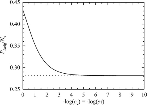35) where l is expressed in multiples of a/2. The key quantity needed to relate measured EFG fluctuation rate to tracer jump rate in Equation 1 is the quotient $P_{\mathrm{\Delta }\mathrm{E}\mathrm{F}\mathrm{G}}/N_{\mathrm{e}}$, which is shown in Figure 5 as a function of vacancy concentration. Treatment of vacancy motion as a discrete random walk and choice of the form of Equation 6 come from the assumption that vacancy concentration is small. Calculations, therefore, are unlikely to be reliable for values of c_v larger than about 10⁻². Nevertheless, the numerical calculations are well-defined up to c_v = 1, and the full range $0\le c_{\mathrm{v}}\le 1$ is shown in the figure. As can be seen, r will differ from Zc_v w₂ by a factor between about 0.281 and 0.306.

Figure 5. Dependence of $P_{\mathrm{\Delta }\mathrm{E}\mathrm{F}\mathrm{G}}/N_{\mathrm{e}}$ in Equation 1 as a function of vacancy concentration c_v. The value determined using the time-independent formulation, corresponding to the infinitesimal vacancy concentration limit c_v = 0, is shown as a dashed line.

Discussion

Perturbed angular correlation spectroscopy has been used to study cadmium movement in a number of L1₂-structured compounds: RIn₃ [17,18,28], RSn₃ [19], RGa₃ [20], and RPd₃ [21] where R = rare earth element. In reports of these studies, it was assumed that there was a one-to-one correspondence between a tracer jump and an EFG reorientation so that w = 2r where $w=Z{c}_{\mathrm{v}}{w}_2$ is the total tracer jump rate [17,28]. According to Equation 1, $w=r{N}_{\mathrm{e}}/P_{\mathrm{\Delta }\mathrm{E}\mathrm{F}\mathrm{G}}$ so that tracer-jump rates deduced in the earlier work likely underestimate actual values by a factor $2P_{\mathrm{\Delta }\mathrm{E}\mathrm{F}\mathrm{G}}/N_{\mathrm{e}}$.

For the case of self-diffusion on the Cu sublattice, the present work gives the factor $P_{\mathrm{\Delta }\mathrm{E}\mathrm{F}\mathrm{G}}/N_{\mathrm{e}}$ to be between about 0.281 and 0.306. Caution should be exercised when using the present results to translate EFG fluctuation rates measured in previous PAC studies [17–21] to tracer jump rates, because cadmium was an impurity diffuser. Further work is needed to develop methods needed to calculate $P_{\mathrm{\Delta }\mathrm{E}\mathrm{F}\mathrm{G}}/N_{\mathrm{e}}$ for the impurity-diffusion case. In the meantime, the present results are directly applicable to PAC work aiming to measure In-jump rates in RIn₃ [29] and Cd-jump rates in NbCd₃ [30] closely related to the previous experiments.

As proposed previously [17, 28–32], independent measurements of tracer movement using PAC and conventional diffusion measurements will allow experimental determination of the diffusion correlation factor. For example, the diffusion coefficient D is related to the tracer-vacancy exchange rate w₂ for self-diffusion on the Cu sublattice of the Cu₃Au structure by $D=\frac{2}{3}f{a}^2{c}_{\mathrm{v}}{w}_2$ where a is the lattice parameter [33], which can be expressed $D=\frac{1}{12}f{a}^{2}w$ [17]. Because PAC does not measure the tracer jump rate directly, instead measuring the EFG reorientation rate r, the diffusion coefficient can be found via $f=12a^{-2}D{r}^{-1}{P}_{\mathrm{\Delta }\mathrm{E}\mathrm{F}\mathrm{G}}/N_{\mathrm{e}}$ using the quantity $P_{\mathrm{\Delta }\mathrm{E}\mathrm{F}\mathrm{G}}/N_{\mathrm{e}}$ provided by the present work.

PAC measurement of atomic jump rates may also provide the opportunity to measure stochastic-resonance (SR) effects. SR is amplification of a time-dependent, external driving potential by background noise [34]. In the context of a random-walking particle that must overcome a potential barrier to make a jump, SR can influence jump rates in effects known as resonant activation [35] and noise enhanced stability [36] for increased and decreased rates, respectively. A recent article by Spagnolo et al. [37] provides a good source of citations to many important papers in the field. Kallunki, Dube, and Ala-Nissila have shown that a useful qualitative, theoretical description of the SR effect on a random-walker in a 1-D periodic potential can be derived by using an appropriate time-dependent jump rate in the Master equation [38,39]. It may, therefore, be possible to estimate the impact that SR will have on measurement of atomic jump rates using hyperfine methods by using a time-dependent jump rate, such as the Kramers [40] or closely-related rates [41], instead of inverse residence time in the time-dependent vacancy-encounter model. This would necessitate reformulation of expressions needed to calculate P_ΔEFG/N_e starting with new functional forms for w_k(t) in Equation 2 and f(c_v,t) in Equation 6.

Summary

In a vacancy-mediated diffusion process, tracers jump via a correlated random walk. EFGs experienced by tracer nuclei will change when tracers jump among lattice sites with orientationally inequivalent site symmetries. When tracers jump with a rate comparable to the inverse characteristic timescale of the hyperfine method used to measure the EFGs, the EFG fluctuations induce a damping or line broadening in spectra. Measurement of the degree of damping or broadening allows determination of EFG fluctuation rate. For relatively low vacancy concentration and negligible interaction between vacancies and tracer, the residence time of vacancies needs to be much smaller than the timescale of the hyperfine method so that EFG fluctuations induced by tracer jumps are at the same timescale of, and therefore observable by, the hyperfine method. This means that multiple tracer-vacancy exchanges can occur during a single tracer-vacancy encounter, and a tracer can wind up in a lattice site with the same EFG it started. Such encounters do not contribute to damping or line-broadening and go undetected by the hyperfine method.

In a high-symmetry crystal system for which all vacancy jumps have same jump frequency, $r=P_{\mathrm{\Delta }\mathrm{E}\mathrm{F}\mathrm{G}}Z{c}_{\mathrm{v}}{w}_2/N_{\mathrm{e}}$ where r is the EFG fluctuation rate, Z is the coordination number, c_v is the vacancy concentration, w₂ is the vacancy-tracer exchange rate, P_ΔEFG is the probability that a vacancy encounter leads to a particular type of EFG change, and N_e is the average number of tracer-vacancy exchanges per encounter. Using a time-dependent, random-walk analysis of tracer displacement probabilities in a vacancy encounter model, the quantity P_ΔEFG/N_e was calculated for the special case of self-diffusion on the Cu sublattice of the Cu₃Au crystal structure. It was found to range between about 0.281 for infinitesimal vacancy concentration and 0.306 for c_v = 0.01, which is a reasonable upper limit for the range of validity of these calculations. The ramifications of this result for using EFG fluctuation rates measured using PAC and other hyperfine methods to deduce tracer jump rates and measure correlation factors in conjunction with conventional diffusion experiments and the possibility to investigate stochastic resonance effects were discussed.

Acknowledgements

The authors gratefully acknowledge helpful discussions with Gary S. Collins, Randy Newhouse, and William E. Evenson.

Disclosure statement

No potential conflict of interest was reported by the authors.

ORCID

Matthew O. Zacate http://orcid.org/0000-0001-6277-6814

Additional information

Funding

This work was supported by the National Science Foundation [Grants DMR 06-06006 and DMR 15-08189].

Appendix

Using expressions from Equations 24 and 25, Equation 26 can be expressed(A1) $\begin{array}{rl}{\mathbf{P}}_{}\left(\mathbf{v},{\mathbf{v}}_1:z\right)=& \frac{a^3}{{\left(2\pi \right)}^3}\int \int {\int }_{-\pi /a}^{\pi /a}\frac{\exp \left(i\phi \cdot \left(\mathbf{v}-{\mathbf{v}}_1\right)\right)d\phi }{D\left(\phi \right)}\\ & \times \left(\begin{array}{c}1-\frac{1}{4}{z}^2{\cos }^2\left(a{\phi }_y/2\right){\cos }^2\left(a{\phi }_z/2\right)\\ \frac{1}{8}z\cos \left(a{\phi }_x/2\right)\cos \left(a{\phi }_y/2\right)\left[4+z+z\cos \left(a{\phi }_z\right)\right]\\ \frac{1}{8}z\cos \left(a{\phi }_x/2\right)\cos \left(a{\phi }_z/2\right)\left[4+z+z\cos \left(a{\phi }_y\right)\right]\end{array}\right).\end{array}$(A1) In order to calculate the terms $Q_{ij}^{\gamma \beta \alpha }\left(s\right)$ needed for calculating numbers of jumps per encounter and atomic jump probabilities, values of $\mathbf{P}\left(\mathbf{v},{\mathbf{v}}_1:z\right)$ are required only for those v and v ₁ that correspond to first neighbour jump vectors. It simplifies discussion of symmetry to note that according to Equation A1, $\mathbf{P}\left(\mathbf{v}-{\mathbf{v}}_1,\mathbf{0}:z\right)=\mathbf{P}\left(\mathbf{v},{\mathbf{v}}_1:z\right)$.

Symmetry of the L1₂ structure reveals the following equalities among elements of $\mathbf{P}\left(\mathbf{v},\mathbf{0}:z\right)$.

• $P^{Z,Z}\left(\left(0,0,\left|a\right|\right),\mathbf{0}:z\right)=P^{Y,Y}\left(\left(0,\left|a\right|,0\right),\mathbf{0}:z\right)=P^{X,X}\left(\left(\left|a\right|,0,0\right),\mathbf{0}:z\right)$

• $P^{Y,Y}\left(\left(\left|a\right|,0,0\right),\mathbf{0}:z\right)=P^{Y,Y}\left(\left(0,0,\left|a\right|\right),\mathbf{0}:z\right)=P^{Z,Z}\left(\left(0,\left|a\right|,0\right),\mathbf{0}:z\right)=P^{Z,Z}\left(\left(\left|a\right|,0,0\right),\mathbf{0}:z\right)=P^{X,X}\left(\left(0,\left|a\right|,0\right),\mathbf{0}:z\right)=P^{X,X}\left(\left(0,0,\left|a\right|\right),\mathbf{0}:z\right)$

• $P^{Y,Y}\left(\left(\left|a\right|,0,\left|a\right|\right),\mathbf{0}:z\right)=P^{Z,Z}\left(\left(\left|a\right|,\left|a\right|,0\right),\mathbf{0}:z\right)=P^{X,X}\left(\left(0,\left|a\right|,\left|a\right|\right),\mathbf{0}:z\right)$

• $P^{Y,Y}\left(\left(0,\left|a\right|,\left|a\right|\right),\mathbf{0}:z\right)=P^{Y,Y}\left(\left(\left|a\right|,\left|a\right|,0\right),\mathbf{0}:z\right)=P^{Z,Z}\left(\left(\left|a\right|,0,\left|a\right|\right),\mathbf{0}:z\right)=P^{Z,Z}\left(\left(0,\left|a\right|,\left|a\right|\right),\mathbf{0}:z\right)=P^{X,X}\left(\left(\left|a\right|,0,\left|a\right|\right),\mathbf{0}:z\right)=P^{X,X}\left(\left(\left|a\right|,\left|a\right|,0\right),\mathbf{0}:z\right)$

• $P^{X,Y}\left(\left(\left|\frac{a}{2}\right|,\left|\frac{a}{2}\right|,0\right),\mathbf{0}:z\right)=P^{X,Z}\left(\left(\left|\frac{a}{2}\right|,0,\left|\frac{a}{2}\right|\right),\mathbf{0}:z\right)=P^{Y,Z}\left(\left(0,\left|\frac{a}{2}\right|,\left|\frac{a}{2}\right|\right),\mathbf{0}:z\right)=P^{Z,Y}\left(\left(0,\left|\frac{a}{2}\right|,\left|\frac{a}{2}\right|\right),\mathbf{0}:z\right)=P^{Y,X}\left(\left(\left|\frac{a}{2}\right|,\left|\frac{a}{2}\right|,0\right),\mathbf{0}:z\right)=P^{Z,X}\left(\left(\left|\frac{a}{2}\right|,0,\left|\frac{a}{2}\right|\right),\mathbf{0}:z\right)$

• $P^{X,Y}\left(\left(\left|\frac{a}{2}\right|,\left|\frac{a}{2}\right|,\left|a\right|\right),\mathbf{0}:z\right)=P^{X,Z}\left(\left(\left|\frac{a}{2}\right|,\left|a\right|,\left|\frac{a}{2}\right|\right),\mathbf{0}:z\right)=P^{Y,Z}\left(\left(\left|a\right|,\left|\frac{a}{2}\right|,\left|\frac{a}{2}\right|\right),\mathbf{0}:z\right)=P^{Z,Y}\left(\left(\left|a\right|,\left|\frac{a}{2}\right|,\left|\frac{a}{2}\right|\right),\mathbf{0}:z\right)=P^{Y,X}\left(\left(\left|\frac{a}{2}\right|,\left|\frac{a}{2}\right|,\left|a\right|\right),\mathbf{0}:z\right)=P^{Z,X}\left(\left(\left|\frac{a}{2}\right|,\left|a\right|,\left|\frac{a}{2}\right|\right),\mathbf{0}:z\right)$

It is, therefore, sufficient to evaluate just 7 unique terms, including $P_{}^{X,X}\left(\left(0,0,0\right),\mathbf{0}:z\right)$.

Integrals of the first four unique terms, $P_{}^{X,X}\left(\left(\left|a\right|,0,0\right),\mathbf{0}:z\right)$, $P_{}^{X,X}\left(\left(0,0,\left|a\right|\right),\mathbf{0}:z\right)$, $P_{}^{X,X}\left(\left(0,\left|a\right|,\left|a\right|\right),\mathbf{0}:z\right)$, and $P_{}^{X,X}\left(\left(\left|a\right|,\left|a\right|,0\right),\mathbf{0}:z\right)$, and $P_{}^{X,X}\left(\left(0,0,0\right),\mathbf{0}:z\right)$ are evaluated by writing the first vector as $\mathbf{v}=\left(\frac{l}{2}a,\frac{m}{2}a,\frac{n}{2}a\right)$ for even l, m, and n. The integral can then be written(A2) $\begin{array}{rl}{P}^{X,X}\left(\mathbf{v},\mathbf{0}:z\right)=& \frac{1}{{\left(2\pi \right)}^3}\int \int {\int }_{-\pi }^{\pi }\frac{\exp \left(i\mathbf{\Phi }\cdot \left(\frac{l}{2},\frac{m}{2},\frac{n}{2}\right)\right)}{D\left(\mathbf{\Phi }\right)}d{\mathrm{\Phi }}_{x}d{\mathrm{\Phi }}_{y}d{\mathrm{\Phi }}_z\\ & \times \left(1-\frac{1}{4}{z}^2{\cos }^2\left({\mathrm{\Phi }}_y/2\right){\cos }^2\left({\mathrm{\Phi }}_z/2\right)\right)\end{array}$(A2) where $\mathbf{\Phi }=a\phi$ and(A3) $\begin{array}{rl}D\left(\mathbf{\Phi }\right)=& 1-\frac{1}{4}{z}^2{\cos }^2\left({\mathrm{\Phi }}_y/2\right){\cos }^2\left({\mathrm{\Phi }}_z/2\right)-\frac{1}{4}{z}^2{\cos }^2\left({\mathrm{\Phi }}_x/2\right)\\ & \times \left[{\cos }^2\left({\mathrm{\Phi }}_y/2\right)+{\cos }^2\left({\mathrm{\Phi }}_z/2\right)+z{\cos }^2\left({\mathrm{\Phi }}_y/2\right){\cos }^2\left({\mathrm{\Phi }}_z/2\right)\right].\end{array}$(A3) The integral over ${\mathrm{\Phi }}_x$ can be performed analytically to get(A4) $\begin{array}{rl}{P}^{X,X}\left(\mathbf{v},\mathbf{0}:z\right)=& \frac{1}{{\left(2\pi \right)}^2}{\int }_{-\pi }^{\pi }{\int }_{-\pi }^{\pi }d{\mathrm{\Phi }}_{y}d{\mathrm{\Phi }}_z\exp \left(\frac{1}{2}i\left(m{\mathrm{\Phi }}_y+n{\mathrm{\Phi }}_z\right)\right)\times \\ & \pm \sqrt{\frac{N}{N-M}}{\left(\frac{2N-M\mp 2\sqrt{N\left(N-M\right)}}{M}\right)}^{\frac{l}{2}}\end{array}$(A4) where $N=1-\frac{1}{4}{z}^2{\cos }^2\left({\mathrm{\Phi }}_y/2\right){\cos }^2\left({\mathrm{\Phi }}_z/2\right)$ and $M=\frac{1}{4}{z}^2[{\cos }^2\left({\mathrm{\Phi }}_y/2\right)+{\cos }^2\left({\mathrm{\Phi }}_z/2\right)+$ $z{\cos }^2\left({\mathrm{\Phi }}_y/2\right){\cos }^2\left({\mathrm{\Phi }}_z/2\right)]$.

Integrals of the remaining two terms, $P^{Y,X}\left(\left(\left|\frac{a}{2}\right|,\left|\frac{a}{2}\right|,0\right),\mathbf{0}:z\right)$ and $P^{Y,X}\left(\left(\left|\frac{a}{2}\right|,\left|\frac{a}{2}\right|,\left|a\right|\right),\mathbf{0}:z\right)$ can be evaluated similarly using a combination of analytical and numerical integration. In these cases, the non-zero vector can be written $\mathbf{v}=\left(\frac{l}{2}a,\frac{m}{2}a,\frac{n}{2}a\right)$ for l = m = 1 and even n, specifically n = 0 or n = 2. The needed integrals can be written(A5) $\begin{array}{rl}{\mathbf{P}}_{}\left(\mathbf{v},\mathbf{0}:z\right)=& \frac{1}{{\left(2\pi \right)}^3}\int \int {\int }_{-\pi }^{\pi }\frac{\exp \left(i\mathbf{\Phi }\cdot \left(\frac{l}{2},\frac{m}{2},\frac{n}{2}\right)\right)}{D\left(\mathbf{\Phi }\right)}d{\mathrm{\Phi }}_{x}d{\mathrm{\Phi }}_{y}d{\mathrm{\Phi }}_z\\ & \times \left(\frac{1}{8}z\cos \left({\mathrm{\Phi }}_x/2\right)\cos \left({\mathrm{\Phi }}_y/2\right)\left[4+z+z\cos \left({\mathrm{\Phi }}_z\right)\right]\right).\end{array}$(A5) with(A6) $\begin{array}{rl}D\left(\mathbf{\Phi }\right)=& 1-\frac{1}{4}{z}^2{\cos }^2\left({\mathrm{\Phi }}_x/2\right){\cos }^2\left({\mathrm{\Phi }}_y/2\right)-\frac{1}{4}{z}^2{\cos }^2\left({\mathrm{\Phi }}_z/2\right)\\ & \times \left[{\cos }^2\left({\mathrm{\Phi }}_x/2\right)+{\cos }^2\left({\mathrm{\Phi }}_y/2\right)+z{\cos }^2\left({\mathrm{\Phi }}_x/2\right){\cos }^2\left({\mathrm{\Phi }}_y/2\right)\right].\end{array}$(A6) It is useful to define $N^{\mathrm{\prime }}=1-\frac{1}{4}{z}^2{\cos }^2\left({\mathrm{\Phi }}_x/2\right){\cos }^2\left({\mathrm{\Phi }}_y/2\right)$ and $M^{\mathrm{\prime }}=\frac{1}{4}{z}^2\left[{\cos }^2\left({\mathrm{\Phi }}_x/2\right)+{\cos }^2\left({\mathrm{\Phi }}_y/2\right)+z{\cos }^2\left({\mathrm{\Phi }}_x/2\right){\cos }^2\left({\mathrm{\Phi }}_y/2\right)\right]$ in order to integrate over ${\mathrm{\Phi }}_z$ analytically. This gives for n = 0:(A7a) $\begin{array}{rl}{P}^{Y,X}\left(\mathbf{v},\mathbf{0}:z\right)=& \frac{1}{{\left(2\pi \right)}^2}{\int }_{-\pi }^{\pi }{\int }_{-\pi }^{\pi }d{\mathrm{\Phi }}_{x}d{\mathrm{\Phi }}_y\exp \left(\frac{1}{2}i\left(l{\mathrm{\Phi }}_x+m{\mathrm{\Phi }}_y\right)\right)\times \\ & \pm \frac{1}{2}\frac{\sqrt{1-N^{\mathrm{\prime }}}}{\sqrt{N^{\mathrm{\prime }}\left(N^{\mathrm{\prime }}-M^{\mathrm{\prime }}\right)}}\frac{2M^{\mathrm{\prime }}+N^{\mathrm{\prime }}z-z\sqrt{N^{\mathrm{\prime }}\left(N^{\mathrm{\prime }}-M^{\mathrm{\prime }}\right)}}{M^{\mathrm{\prime }}},\end{array}$(A7a) and for n = 2:(A7b) $\begin{array}{rl}& P^{Y,X}\left(\mathbf{v},\mathbf{0}:z\right)=\frac{1}{{\left(2\pi \right)}^2}{\int }_{-\pi }^{\pi }{\int }_{-\pi }^{\pi }d{\mathrm{\Phi }}_{x}d{\mathrm{\Phi }}_y\exp \left(\frac{1}{2}i\left(l{\mathrm{\Phi }}_x+m{\mathrm{\Phi }}_y\right)\right)\times \\ & \pm \frac{1}{4}\frac{\sqrt{1-N^{\mathrm{\prime }}}}{\sqrt{N^{\mathrm{\prime }}\left(N^{\mathrm{\prime }}-M^{\mathrm{\prime }}\right)}}\frac{1}{{M^{\mathrm{\prime }}}^2}\left\{\right(4+z)M^{\mathrm{\prime }}\left(2N^{\mathrm{\prime }}-M^{\mathrm{\prime }}-2\sqrt{N^{\mathrm{\prime }}\left(N^{\mathrm{\prime }}-M^{\mathrm{\prime }}\right)}\right)\\ & +\frac{z}{2}{M^{\mathrm{\prime }}}^2+\frac{z}{2}{\left(2\sqrt{N^{\mathrm{\prime }}\left(N^{\mathrm{\prime }}-M^{\mathrm{\prime }}\right)}-2N^{\mathrm{\prime }}+M^{\mathrm{\prime }}\right)}^2\}.\end{array}$(A7b)

Final calculation of $P^{X,X}\left(\mathbf{v},\mathbf{0}:z\right)$ and $P^{Y,X}\left(\mathbf{v},\mathbf{0}:z\right)$ requires use of a numerical integration method. Equations A4 and A7 can be calculated conveniently, for example, using the default global adaptive numerical integration settings in Mathematica [42]. Results for selected values of c_v are given in Table A1.

Table A1. $P^{X,X}\left(\mathbf{v},\mathbf{0}:z\right)$ and $P^{Y,X}\left(\mathbf{v},\mathbf{0}:z\right)$ calculated for selected values of c_v.

v	cv = 1	cv = 0.1	cv = 0.01	cv = 0.001	cv = 0.0001	cv = 0
$\left(0,0,0\right)$	1.038933676	1.218359066	1.375662592	1.442330467	1.465285302	1.476212780
$\left(\left|a\right|,0,0\right)$	0.019969754	0.127155396	0.247143103	0.307297226	0.329476024	0.340312227
$\left(0,0,\left|a\right|\right)$	0.01167128	0.094202205	0.205253117	0.264248709	0.28630764	0.297130466
$\left(0,\left|a\right|,\left|a\right|\right)$	0.001854867	0.04115058	0.125789296	0.179716833	0.201150077	0.211898417
$\left(\left|a\right|,\left|a\right|,0\right)$	0.006077012	0.058861425	0.148817201	0.203459478	0.224967229	0.235723887
$\left(\left|\frac{a}{2}\right|,\left|\frac{a}{2}\right|,0\right)$	0.077867353	0.240194999	0.379419351	0.442772803	0.465331872	0.476212825
$\left(\left|\frac{a}{2}\right|,\left|\frac{a}{2}\right|,\left|a\right|\right)$	0.006745612	0.067373912	0.164996767	0.221421536	0.243163615	0.253948752

References

- J. Philibert, Atom Movements: Diffusion and Mass Transport in Solids, Éditions de Physique, Les Ulis, 1991.
- P. Heitjans and J. Kärger (eds.), Diffusion in Condensed Matter, Springer-Verlag, Berlin, 2005.
- G. Schatz and A. Weidinger, Nuclear Condensed Matter Physics, John Wiley and Sons, Ltd, West Sussex, 1996.
- W.E. Evenson, Defect-related dynamic hyperfine interactions, in Proceedings of the XXXIV Zakopane School of Physics: Condensed Matter Studies by Nuclear Methods, 2000.
- S. Dattagupta, Study of time-dependent hyperfine interactions by PAC, Mössbauer effect, μSR and NMR: A review of stochastic models. Hyperfine Interact. 11 (1981), pp. 77–126. doi: 10.1007/BF01026470
- R. Kubo, Stochastic theory of resonance absorption. J. Phys. Soc. Jpn. 9 (1954), pp. 935–944. doi: 10.1143/JPSJ.9.935
- P.W. Anderson, A Mathematical model for the narrowing of spectral lines by exchange or motion. J. Phys. Soc. Jpn. 9 (1954), pp. 316–339. doi: 10.1143/JPSJ.9.316
- J. Roberts and R.M. Lynden-Bell, Line shapes of a tumbling triplet. Mol. Phys. 21(4) (1971), pp. 689–699. doi: 10.1080/00268977100101841
- S. Dattagupta and M. Blume, Stochastic theory of line shape. II. Nonsecular effects in the EPR spectrum of carbon dioxide(-) ions in calcite. Phys Rev B 10(11) (1974), pp. 4551–4559. doi: 10.1103/PhysRevB.10.4551
- M.O. Zacate and W.E. Evenson, Stochastic hyperfine interactions modeling library. Comput Phys Commun 182 (2011), pp. 1061–1077. doi: 10.1016/j.cpc.2010.12.042
- H. Muhammed, M.O. Zacate, and W.E. Evenson, Simulation of PAC spectra for spin 5/2 probes diffusing via a simple vacancy mechanism in Cu3Au-structured intermetallic compounds. Hyperfine Interact. 177(1–3) (2007), pp. 45–49. doi: 10.1007/s10751-008-9620-1
- J.R. Castle, M.O. Zacate, and W.E. Evenson, Realistic models of stochastically varying hyperfine interactions caused by vacancy diffusion in L12-structured compounds. Hyperfine Interact. 222(1–3) (2013), pp. 109–120. doi: 10.1007/s10751-012-0695-3
- C.A. Sholl, Diffusion correlation factors and atomic displacements for the vacancy mechanism. J. Phys. C: Solid State Phys. 14 (1981), pp. 2723–2729. doi: 10.1088/0022-3719/14/20/011
- D. Wolf, Theory of correlation effects in diffusion. NATO ASI Ser., Ser. B 97( Proceedings of a NATO Advanced Study Institute on Mass Transport in Solids) (1983), pp. 149–168.
- J. Baker, C.J. Girard and C.A. Sholl, The time dependence of an atom-vacancy encounter due to the vacancy mechanism of diffusion. Philos. Mag. A 74(2) (1996), pp. 543–552. doi: 10.1080/01418619608242161
- N. Dasenbrock-Gammon and M.O. Zacate, A comment on Baker et al. ‘The time dependence of an atom-vacancy encounter due to the vacancy mechanism of diffusion’. Philos. Mag. 97(15) (2017), pp. 1238–1242. doi: 10.1080/14786435.2017.1293861
- M.O. Zacate, A. Favrot, and G.S. Collins, Atom movement in In3La studied via nuclear quadrupole relaxation. Phys. Rev. Lett. 92 (2004), pp. 225901. doi: 10.1103/PhysRevLett.92.225901
- G.S. Collins, X. Jiang, J.P. Bevington, F. Selim, and M.O. Zacate, Change of diffusion mechanism with lattice parameter in the series of lanthanide indides having L12 structure. Phys. Rev. Lett. 102 (2009), pp. 155901. doi: 10.1103/PhysRevLett.102.155901
- M. Lockwood, B. Norman, R. Newhouse, and G.S. Collins, Comparison of jump frequencies of 111In/Cd tracer atoms in Sn3R and In3R phases having the L12 structure (R=rare earth). Defect Diffusion Forum 311 (2011), pp. 159–166. doi: 10.4028/www.scientific.net/DDF.311.159
- X. Jiang, M.O. Zacate, and G.S. Collins, Jump frequencies of Cd tracer atoms in L12 lanthanide gallides. Defect and Difffusion Forum 725 (2009), pp. 289.
- Q. Wang and G.S. Collins, Nuclear quadrupole interactions of 111In/Cd solute atoms in a series of rare-earth palladium alloys. Hyperfine Interact. 221 (2013), pp. 85–98. doi: 10.1007/s10751-012-0686-4
- H. Winkler and E. Gerdau, γγ-Angular correlations peturbed by stochastic fluctuating fields. Zeitschrift für Physik 262 (1973), pp. 363–376. doi: 10.1007/BF01394538
- A. Baudry and P. Boyer, Approximation of the Blume's stochastic model by asymptotic models for PAC relaxation analysis. Hyperfine Interact. 35 (1987), pp. 803–806. doi: 10.1007/BF02394496
- W.E. Evenson, J.A. Gardner, R. Wang, H.-T. Su and A.G. McKale, PAC analysis of defect motion by Blume's stochastic model for I=5/2 electric quadrupole interactions. Hyperfine Interact. 62 (1990), pp. 283–300. doi: 10.1007/BF02397709
- M.O. Zacate and W.E. Evenson, Comparison of XYZ model fitting functions for 111Cd in In3La. Hyperfine Interact. 158(1–4) (2005), pp. 329–332. doi: 10.1007/s10751-005-9049-8
- M.O. Zacate and W.E. Evenson, Stochastic hyperfine interactions modeling library - version 2. Comput. Phys. Commun. 199 (2016), pp. 180–181. doi: 10.1016/j.cpc.2015.10.013
- C.A. Sholl, Atomic displacements due to the vacancy mechanism. Philos. Mag. A 65(3) (1992), pp. 749–756. doi: 10.1080/01418619208201547
- M.O. Zacate, A. Favrot and G.S. Collins, Erratum: atom movement in In3La studied via nuclear quadrupole relaxation [Phys. Rev. Lett. 92, 225901 (2004)]. Phys. Rev. Lett. 93(4) (2004), p. 049903. doi: 10.1103/PhysRevLett.93.049903
- M.O. Zacate, M. Deicher, K. Johnston, J. Lehnert, F. Strauss and G.S. Collins, Diffusion in Intermetallic Compounds Studied Using Short-Lived Radioisotopes. CERN Document Server: Preprints, Vols. CERN-INTC-2011-010/INTC-P-294 (2011), pp. 1–11.
- M.O. Zacate, J. Schell and J.G.M. Correia, Direct Measurement of self diffusion jump rates in an intermetallic compound. CERN Document Server: Preprints, Vols. CERN-INTC-2016-053; CERN-INTC-2017-014; INTC-P-483 (2016), pp. 1–11.
- G.S. Collins, A. Favrot, L. Kang, D. Solodovnikov and M.O. Zacate, Diffusion in Intermetallic compounds studied using nuclear quadrupole relaxation. Defect and Diffusion Forum 237–240 (2005), pp. 195–200. doi: 10.4028/www.scientific.net/DDF.237-240.195
- G.S. Collins, A. Favrot, L. Kang, E.R. Nieuwenhuis, D. Solodovnikov, J. Wang and M.O. Zacate, PAC probes as diffusion tracers in compounds. Hyperfine Interact. 159(1–4) (2005), pp. 1–8. doi: 10.1007/s10751-005-9073-8
- T. Ito, S. Ishioka, and M. Koiwa, Correlation factor for diffusion via sublattice vacancy mechanism in the L12-type ordered alloy. Philos. Mag. A 62(5) (1990), pp. 499–510. doi: 10.1080/01418619008244915
- L. Gammaitoni, P. Hänggi, P. Jung and F. Marchesoni, Stochastic resonance. Rev. Mod. Phys. 70(1) (1998), pp. 223–287. doi: 10.1103/RevModPhys.70.223
- C.R. Doering and J.C. Gadoua, Resonant activation over a fluctuating barrier. Phys. Rev. Lett. 69(16) (1992), pp. 2318–2321. doi: 10.1103/PhysRevLett.69.2318
- A.A. Dubkov, N.V. Agudov and B. Spagnolo, Noise-enhanced stability in fluctuating metastable states. Phys Rev E 69 (2004), p. 061103/1-7. doi: 10.1103/PhysRevE.69.061103
- B. Spagnolo, C. Guarcello, L. Magazzù, A. Carollo, D.P. Adorno and D. Valenti, Nonlinear relaxation phenomena in metastable condensed matter systems. Entropy 19(1) (2017), p. 20/1–26. doi: 10.3390/e19010020
- J. Kallunki, M. Dubé and T. Ala-Nissila, Stochastic resonance and diffusion in periodic potentials. J. Phys.: Condens. Matter 11 (1999), pp. 9841–9849.
- J. Kallunki, M. Dubé and T. Ala-Nissila, Adatom dynamics in a periodic potential under time-periodic bias. Surf. Sci. 460 (2000), pp. 39–48. doi: 10.1016/S0039-6028(00)00490-8
- H.A. Kramers, Brownian motion in a field of force and the diffusion model of chemical reactions. Physica 7(4) (1940), pp. 284–304. doi: 10.1016/S0031-8914(40)90098-2
- P. Jung, Thermal activation in bistable systems under periodic forces. Z. Phys. B Condens. Matter 76 (1989), pp. 521–535. doi: 10.1007/BF01307904
- Mathematica, Version 11.0.1.0, Wolfram Research, Inc., Champaign, IL, 2016.