Modelling of short-range ordering kinetics in dilute multicomponent substitutional solid solutions

ABSTRACT

Short-range ordering as the formation of couples and pairs between solutes is affected by their formation energies. This is not reflected in the standard regular solution model. Here, we present a new thermodynamic model which accounts for the dependence of the molar Gibbs energy on the concentrations of couples and pairs and their formation energies. The model treats kinetics of couples and pairs formation controlled by diffusion. This new model uses tracer diffusion coefficients of solutes and bond formation energies, which can be taken from ab initio calculations. Insofar, the current concept bridges the gap between ab initio methods and non-equilibrium thermodynamics. The reliability of the model is checked by comparison with kinetic Monte Carlo simulations. The model is applied to an Al-Mg-Si-Cu system. Finally, the configurational entropy for a binary system evaluated with the current model is compared with Bethe’s approximation, which allows estimating of applicability limits of the current model.

KEYWORDS:

• Order
• kinetics
• thermodynamics
• solid solutions
• modelling
• couples and pairs

1. Introduction and motivation

Matrices of traditional structural materials as those based on Mg alloyed with Zn, Al [1,2], on Al alloyed with Mg, Si, Cu [3–5] or low-alloyed steels [6,7] can be considered as substitutional solid solutions with Mg, Al or Fe as solvents and several dilute substitutional solutes. The amounts of interstitial alloying elements in the alloys are mostly insignificant or they are substantially reduced in the matrix by precipitation. The substitutional solutes in the matrix can play an important role to assure an increase in strength as well as fracture and corrosion/oxidation resistance necessary for practical applications. The formation of pairs of substitutional elements plays here a remarkable role and has been investigated experimentally already several decades ago, see e.g. the study by Masanskii et al. [8]. Obviously, the experimental data were usually interpreted by the Krivoglaz–Clapp–Moss approximation. Here we refer to the three papers by Clapp and Moss [9–11] and the book by Krivoglaz [12]; all of these works were already published more than fifty years ago!

Although Al- or Mg-based alloys and particularly Fe-based low-alloyed steels are of enormous practical relevance, the proper treatment of the actual arrangement of atoms in the lattice still represents a demanding scientific topic. Considering the experimental research, significant progress can be observed, e.g. for Al-based alloys, as studied e.g. in [4,13]. With respect to the atomic arrangement in the lattice and microstructural evolution, however, most of the numerous publications deal only with the equilibrium state of such alloys by evaluating Gibbs energies of individual phases, see established concepts such as Calphad [14] and a corresponding software Thermocalc [15]. The precipitation kinetics is treated by rather new software Matcalc [16]. The calculation of the Gibbs energy of a solid-solution matrix is usually based on the widely accepted Bragg–Williams [17] approximation for configurational entropy of a mixture by using the assumption that the atomic arrangement of all components in the lattice is random. Then the numbers of couples (Cs), consisting of two neighbouring solute atoms of different elements and pairs (Ps), consisting of two neighbouring solute atoms of the same element, are given only by an overall chemical composition of the matrix, and are independent of interactions between atoms. In reality, however, the equilibrium numbers of Cs and Ps do depend on interaction energies between atoms of individual solutes and of the solvent. Here we refer to two recent contributions by Svoboda and Fischer, which introduced a so-called self-consistent model for binary systems and later for multicomponent systems [18,19]. This new model takes the formation energies of the Cs and Ps into account and allows formulating equations for calculation of their equilibrium concentrations. Since, however, the equilibrium concentrations depend on the temperature, the system tends towards a new equilibrium state with certain kinetics controlled by diffusion of solute atoms. Thus, in many cases, the solid solution cannot be considered as an equilibrium system, however, with the help of the here introduced model, its temperature history can be reflected. It must also be noted that the short-range ordering leading to formation of Cs and Ps and later to clustering of atoms, see e.g. very recent paper [20], can be considered as decisive step for a nucleation of precipitates.

It is necessary to be noted that there already exist several concepts treating the dependence of Cs and Ps equilibrium concentrations on their interaction energies based on a statistical approach. These concepts allow also expressing the Gibbs energy of the system out of equilibrium characterised by Cs and Ps concentrations as state variables. Such concepts are summarised in Kapoor’s review [21] from 1975 describing in detail the Quasi-chemical Theory developed jointly by Fowler [22], Bethe [23], Guggenheim [24] and Rushbrooke [25] and the Central- (surrounded-) Atom Model developed simultaneously by Lupis and Elliot [26] and by Mathieu et al. [27,28]. Just the physical base of Central- (surrounded-) Atom Model resembles our model, which is, however, treated mathematically in a different way. It is also worth noting that Hillert [29] introduced in 2001 the Compound Energy Formalism, which also utilises the Quasi-chemical Theory in individual sublattices. So it allows the treatment of stoichiometric compounds and their sophisticated description within CALPHAD or FACT-SAGE approaches. The cluster variation method (CVM) has been invented to deal with agglomerates of solute atoms larger than two atoms. As, however, the formalism of CVM is rather complicated, it is not relevant to our problem of dilute systems, where Cs and Ps dominate.

It may be also of interest that short-range ordering is still an attractive topic for experimental research, see the very recent papers on binary substitutional alloys [30,31].

The motivation of this paper is to present a general atomistic-statistical-thermodynamic model for the treatment of kinetics of numbers of Cs and Ps in a dilute multicomponent system under varying temperature in a compact way. In contrast to previous statistical mechanics models, the calculation of Gibbs energy of the system is based on the division of the system into subsystems and application of the established Bragg–Williams approximation to these individual subsystems. The state of the system is then described by concentrations of atoms in Cs and Ps considered as independent internal state variables. The bonding energies are calculated by ab initio methods in a standard way. To determine the kinetics of the system, additionally, only tracer diffusion coefficients of all solute components are needed. Therefore, the model combines ab initio calculations with non-equilibrium thermodynamics and can be utilised for an improved determination of the thermodynamic properties of solid solutions accounting also for their thermal history. It is also necessary to be noted that the present kinetic model allows calculations within well acceptable computation times, which cannot be achieved using other kinetic/atomistic methods. To check the accuracy of the present model the results of simulations are compared with simulations by kinetic Monte Carlo Method with a very good agreement.

2. Method and analysis

The atomistic/thermodynamic description of the state of the multicomponent system and of its Gibbs energy has been worked out very recently [19]. The model introduces a number of variables necessary for evaluation of the total Gibbs energy $G$ of the system. For the sake of compactness and convenient readability of this paper, we repeat the derivation of the leading equations in a simplified and more plausible way and provide some corrections and additional explanations.

2.1. System definition

We assume $n$ substitutional components in a solid solution system of volume $\mathrm{\Omega }$, consisting of one mole of atoms. The vacancies are assumed to be in equilibrium and of a negligible site fraction. The chemical composition is given by overall site fractions $y_i$, $i=1,\dots ,n$, $\sum _{i=1}^n{y}_i=1$ or by concentrations $c_i=y_i/\mathrm{\Omega }$, with component 1 being the solvent and components $i=2,\dots ,n$ being dilute substitutional solutes. The quantities $c_{ij}=c_{ji}$, $i,j=2,\dots ,n,$ $\left[c_i,c_{ij}\right]=\mathrm{m}\mathrm{o}\mathrm{l}/{\mathrm{m}}^3$, denote the concentrations of atoms of component $i$ ($i$-atoms) having a $j$-atom as the nearest neighbour. The assumption of dilute solutes justifies that the concentration of solute atoms with more than one solute atom as the nearest neighbour is negligible compared to $c_{ij}$. The quantities $c_{i1}$, $i=2,\dots ,n$, denote the concentrations of solute $i$-atoms with no solute atom as the nearest neighbour (isolated $i$-atoms) yielding(1) $\sum _{j=1}^n{c}_{ij}=c_i\Rightarrow c_{i1}=c_i-\sum _{j=2}^n{c}_{ij},i=2,\dots ,n.$(1) With $Z$ being the coordination number, the lattice positions can be sorted as those surrounded solely by $Z$ solvent 1-atoms and those surrounded by $Z-1$ solvent 1-atoms and one solute $i$-atom, $i=2,\dots ,n$. The respective amounts of moles of these lattice positions $N_i$, $i=1,\dots ,n$, are given by(2) $N_i=Z{y}_i,i=2,\dots ,n$(2)

and, since the total amount of lattice positions is 1 mol, by(3) $N_1=1-\sum _{i=2}^n{N}_i=1-Z\sum _{i=2}^n{y}_i.$(3) In this way, the system is divided into $n$ $i$-subsystems with ‘weights’ $N_i$, $i=1,\dots ,n$.

2.2. Amount of moles of bonds between solute atoms

The amount of moles $N_{ij}$ of $i-j$ bonds between solute $i$- and $j$-atoms is given as(4) $N_{ij}=N_{ji}=\mathrm{\Omega }{c}_{ij},i,j=2,\dots ,n,i\ne j$(4) and(5) $N_{ii}=\mathrm{\Omega }{c}_{ii}/2,i=2,\dots ,n.$(5) Note that two atoms of component $i$ correspond to one $i-i$ bond. The amount of moles of $1-i$ bonds, $N_{1i}$, is given by the amount of moles of lattice positions of neighbouring $i$-atoms, see Equation (2), reduced by the total amount of moles of these lattice positions occupied by solute atoms, as(6) $N_{1i}=N_{i1}=Z{y}_i-\mathrm{\Omega }\sum _{j=2}^n{c}_{ij},i=2,\dots ,n.$(6) Since the total amount of moles of bonds in the system is $Z/2$, the amount of moles of 1–1 bonds is given by(7) $N_{11}=Z/2-\sum _{i=2}^n\left(\sum _{j=i}^n{N}_{ij}-N_{1i}\right)=Z/2+\mathrm{\Omega }\left(\sum _{i=2}^n\sum _{j=2}^n{c}_{ij}/2-Z\sum _{i=2}^n{c}_i\right).$(7)

2.3. Site fractions in individual subsystems

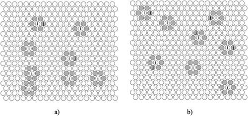
To evaluate the configurational entropy in an individual $i$-subsystem (see Figure 1), $i=1,\dots ,n$, with $N_i$ moles of lattice positions, the site fractions $y_{ij}$ of solute$j$-atoms in the $i$-subsystem must be determined. The amount of moles of solute$j$-atoms neighbouring to a solute $i$-atom (belonging to $i$-subsystem) is given by $c_{ij}\mathrm{\Omega }=c_{ji}\mathrm{\Omega }$, $i=2,\dots ,n,j=2,\dots ,n$. Analogously, the amount of moles of solute$j$-atoms with no solute atom as nearest neighbour (belonging to $1$-subsystem) is given by $c_{j1}\mathrm{\Omega }$, $j=2,\dots ,n$. Then the site fraction $y_{ij}$ is given as the ratio of the amount of moles of solute$j$-atoms, belonging to the $i$-subsystem, and of the amount of moles $N_i$ of lattice positions in the $i$-subsystem, $i=1,\dots ,n$, as(8) $y_{ij}=c_{ji}\mathrm{\Omega }/N_i,i=1,\dots ,n,j=2,\dots ,n.$(8) For the site fractions in the $i$-subsystem, it holds $\sum _{j=1}^n{y}_{ij}=1$. Then the site fraction $y_{i1}$ of the solvent in the $i$-subsystem is given by(9) $y_{i1}=1-\sum _{j=2}^n{y}_{ij},i=1,\dots ,n.$(9)

Figure 1. Two states of the $i$-subsystem (grey lattice positions) generated by eight $i$-atoms with (a) two and (b) five lattice positions occupied by $j$-atoms.

2.4. Determination of configurational entropy

The $i$-subsystem is shown in Figure 1 for its two different states. The number of lattice positions $N_i$ corresponding to the $i$-subsystem remains constant (see Equation (2)), but the location of the $i$-subsystem changes with time as the $i$-atoms diffuse in the system. It is necessary to point out that all positions in the $i$-subsystem are energetically equivalent (see Figure 1). This justifies using the approved and transparent Bragg–Williams approximation for each individual $i$-subsystem. The site fractions $y_{ij}$ of the solutes in the $i$-subsystem are given by Equations (8 and 9), which allow expressing the configurational entropy as a function of the concentrations $c_{ij}=c_{ji}$, $i,j=2,\dots ,n$, considered as independent internal state variables. The equilibrium in the system is then determined by minimising the total Gibbs energy with respect to $c_{ij}$.

The configurational entropy of the system consists of two contributions:

1. the configurational entropy of the $i$-subsystems ($i=1,\dots ,n$) in the system; this is given by the distribution of the $i$-solute atoms in the system. The entropy is given by the Bragg–Williams approximation with $R_g$ being the gas constant as(10) $S_1=-R_g\sum _{i=1}^n\left(y_i\ln y_i\right);$(10)

2. the configurational entropy in individual $i$-subsystems surrounding the central $i$- atom (see Figure 1), given by the Bragg–Williams approximation with $N_i$ representing the ‘weights’ of the subsystem as(11) $S_2=-R_g\sum _{i=1}^n{N}_i\sum _{j=1}^n{y}_{ij}\ln y_{ij}.$(11)

In calculating the entropies $S_1$ and $S_2$ each solute atom plays two roles: the first one as the centre (e.g. atoms i in Figure 1) of the subsystem and the second one as that participating in the subsystem (e.g. atoms j in Figure 1). Therefore, the sum $S_1+S_2$ represents twice the configurational entropy of the system yielding(12) $S=\left(S_1+S_2\right)/2.$(12) With this formulation, we have improved the configurational entropy of a system with couples and pairs, compared to previous formulations in the literature, see also [18,19].

2.5. Determination of Gibbs energy

The total Gibbs energy $G$ of the system can be calculated using the configurational entropy $S$ (Equatioin (12)), the pair-interaction energies ${\epsilon }_{ij}={\epsilon }_{ji}$, $i,j=1,\dots ,n$, $\left[{\epsilon }_{ij}\right]=\mathrm{J}/\mathrm{m}\mathrm{o}\mathrm{l}$, between $i$- and $j$-atoms related to one mole of bonds and $T$ as the absolute temperature, resulting in(13) $G=\overline{G}\left(T\right)-TS+\sum _{i=1}^n\sum _{j=i}^n{\epsilon }_{ij}{N}_{ij}.$(13) The term $\overline{G}\left(T\right)$ represents the part independent of the concentrations $c_{ij}=c_{ji}$. The total Gibbs energy $G$ (Equation (13)) can be reformulated in terms of concentrations $c_{ij}=c_{ji}$, $i,j=2,\dots ,n$, by using Equations (1–9) as(14) $\begin{array}{rl}G& =\overline{G}\left(T\right)+{\epsilon }_{11}Z/2+Z\sum _{i=2}^n\left({\epsilon }_{i1}-{\epsilon }_{11}\right)y_i+\frac{R_{g}T}{2}\sum _{i=1}^n\left(y_i\ln y_i\right)\\ & +\frac{R_{g}T}{2}\mathrm{\Omega }\left(\begin{array}{c}\left(\frac{N_1}{\mathrm{\Omega }}-\sum _{i=2}^n\left(c_i-\sum _{j=2}^n{c}_{ij}\right)\right)\ln \left(1-\frac{\mathrm{\Omega }}{N_1}\sum _{i=2}^n\left(c_i-\sum _{j=2}^n{c}_{ij}\right)\right)\\ +\sum _{i=2}^n\left(\left(c_i-\sum _{j=2}^n{c}_{ij}\right)\ln \left(\left(c_i-\sum _{j=2}^n{c}_{ij}\right)\frac{\mathrm{\Omega }}{N_1}\right)\right)\\ +\sum _{i=2}^n\left(\left(\frac{N_i}{\mathrm{\Omega }}-\sum _{j=2}^n{c}_{ij}\right)\ln \left(1-\sum _{j=2}^n{c}_{ij}\frac{\mathrm{\Omega }}{N_i}\right)+\sum _{j=2}^n{c}_{ij}\ln \left(c_{ij}\frac{\mathrm{\Omega }}{N_i}\right)\right)\end{array}\right)\\ & +\mathrm{\Omega }\left[\sum _{i=2}^n\sum _{j=2}^n\left({\epsilon }_{11}+{\epsilon }_{ij}-{\epsilon }_{i1}-{\epsilon }_{j1}\right)c_{ij}/2\right].\end{array}$(14)

Note that the terms with pre-factor $R_{g}T/2$represent the improved configurational entropy $S=\left(S_1+S_2\right)/2$, which made the present model different from previous formulations. The first two terms in Equation (14) represent the Gibbs energy of a pure solvent, whereas the third term describes the energy contribution of solute atoms surrounded solely by solvent atoms. The fourth configurational entropic term depends on overall chemical composition and the fifth one depends on the internal state variables. The sixth term represents the energy contribution due to the formation of Cs and Ps.

3. Analysis of system equilibrium

3.1. Condition for system equilibrium

The equilibrium in the system corresponds to the minimum of $G$ with respect to the free internal state variables $c_{ij}=c_{ji}$ leading to a set of equations(15) $\frac{\mathrm{\partial }G}{\mathrm{\partial }{c}_{ij}}=0,i=2,\dots ,n,j=i,\dots ,n.$(15) Using Equations (1–11), the derivatives of G read for couples as(16) $\frac{\mathrm{\partial }G}{\mathrm{\partial }{c}_{ij}}=\mathrm{\Omega }\left(\frac{R_{g}T}{2}\ln \left(\frac{y_{ij}{y}_{ji}{y}_{11}^2}{y_{1i}{y}_{1j}{y}_{i1}{y}_{j1}}\right)+E_{ij}\right)\mathrm{f}\mathrm{o}\mathrm{r}i\ne j$(16) and for pairs as(17) $\frac{\mathrm{\partial }G}{\mathrm{\partial }{c}_{ii}}=\frac{\mathrm{\Omega }}{2}\left(R_{g}T\ln \left(\frac{y_{ii}{y}_{11}}{y_{1i}{y}_{i1}}\right)+E_{ii}\right).$(17)

The molar bond formation energies $E_{ij}={\epsilon }_{11}+{\epsilon }_{ij}-{\epsilon }_{i1}-{\epsilon }_{j1}$, $E_{ij}=E_{ji}$, $i,j=2,\dots ,n$ have a clear physical meaning. They express the energy change upon creating one mole of $i-j$ bonds (Cs or Ps) accompanied by the formation of one mole of $1-1$ bonds and loss of one mole of $1-i$ and one mole of $1-j$ bonds. The number of molar bond formation energies $E_{ij}$, being $n\left(n-1\right)/2$, equals to the number of degrees of freedom of the system given by the number of $c_{ij}$. Thus, a one to one correlation exists between $E_{ij}$ and equilibrium values of $c_{ij}$. Note that the last term of $G$, Equation (14), becomes $\mathrm{\Omega }\sum _{i=2}^n\sum _{j=2}^n{E}_{ij}{c}_{ij}/2$.

3.2. Determination of the bond formation energies by ab initio calculations

Bond formation energies in relation to short ordering have been a topic of research during several last decades. We refer to Krivoglaz [12] and his pioneering development of a pair-interaction model based on thermodynamic potentials. However, current atomistic and ab initio methods provide such quantities with much higher accuracy.

The values of $E_{ij}$ are calculated by employing Density Functional Theory-based Vienna Ab initio Simulation Package (VASP) [32]. To demonstrate this procedure we consider an Al-Mg-Si-Cu system. The electron-ion interactions are described using the projector augmented wave method capable pseudopotentials [33], specifically the Al (3s²3p¹), Mg (3s²), Si(3s²3p²) and Cu(3d¹⁰4s¹). The quantum-mechanical electron–electron exchange and correlation interactions are described using generalised gradient approximation as parametrised by Perdew et al. [34], which has been suggested to be superior to local density approximation for Al and Cu, and still reasonably accurate in the case of Si as shown by Haas et al. [35]. The plane-wave cut-off energy of 500 eV and a Monkhorst–Pack mesh of k-points equivalent to 12 × 12 × 12 mesh for a conventional fcc cell ensure the total energy accuracy in the range of meV/at. Clusters of 3 × 3 × 3 supercells containing overall 108 atoms were employed for calculating the molar bond formation energies, $E_{ij}$, as(18) $E_{ij}=N_A\left[E_{\mathrm{t}\mathrm{o}\mathrm{t}}\left(106\mathrm{A}\mathrm{l}+i+j\right)+E_{\mathrm{t}\mathrm{o}\mathrm{t}}\left(108\mathrm{A}\mathrm{l}\right)-E_{\mathrm{t}\mathrm{o}\mathrm{t}}\left(107\mathrm{A}\mathrm{l}+i\right)-E_{\mathrm{t}\mathrm{o}\mathrm{t}}\left(107\mathrm{A}\mathrm{l}+j\right)\right],$(18) where $N_A$ is the Avogadro number and $E_{\mathrm{t}\mathrm{o}\mathrm{t}}\left(\mathrm{X}\right)$ is the total energy of a 108-atom supercell with configuration X (the $i$- and $j$-atoms are the nearest neighbours in the case of 106Al + $i$ + $j$). Negative (positive) values suggest an attractive (repulsive) interaction between atoms $i$ and $j$. In principle, $E_{\mathrm{t}\mathrm{o}\mathrm{t}}\left(\mathrm{X}\right)$ can also be used for evaluation of quantities ${\epsilon }_{ij}$. However, this is not done in the present case since contributions of core electrons are not included in the pseudopotential total energy.

With respect to the calculation of the interaction energies, we refer to the recent paper [36], where a similar atomistic concept has been followed to calculate the pair-interaction energy terms.

3.3. Evaluation of equilibrium chemical potentials

To demonstrate the difference between the established regular solution model and the present short-range ordering concept the chemical potentials of the solutes are calculated for both concepts based on the Equation (A7) in [37] as(19) ${\mu }_i=G+\mathrm{\partial }G/\mathrm{\partial }{y}_i-{\sum }_{j=2}^n{y}_j\mathrm{\partial }G/\mathrm{\partial }{y}_j,i=2,\dots ,n.$(19) The molar Gibbs energy $G$ for given values of $y_i$, $i=2,\dots ,n$, is calculated by using Equation (11) for $c_{ij}=Z{y}_i{y}_j/\mathrm{\Omega }$ following from the assumption of random solution used in the regular solution model and from equilibrium values of $c_{ij}$ calculated by Equation (15). It is expected that all chemical potentials ${\mu }_i^{\mathrm{o}\mathrm{r}\mathrm{d}}$ are lower than ${\mu }_i^{\mathrm{r}\mathrm{e}\mathrm{g}}$, which implies that the molar Gibbs energy calculated from the present short-range ordering concept is lower than that from the regular solution model. Note that the first three terms in Equation (14) vanish in the calculation of the difference ${\mu }_i^{\mathrm{o}\mathrm{r}\mathrm{d}}-{\mu }_i^{\mathrm{r}\mathrm{e}\mathrm{g}}$ and, thus, it depends only on the values of $E_{ij}$, see the last term of Equation (14) and Section 3.1.

4. Analysis of kinetics of Cs and Ps formation

A first attempt to model kinetics of diffusion-controlled formation of Cs, as Mg-Si Cs in a ternary Al-Mg-Si system was reported recently by the authors [38]. This model is based on a defined diffusion zone around a single alloying atom, in which the atoms of the coupling element are collected. The kinetics of the system is determined by means of the thermodynamic extremal principle (TEP) [39]. Kinetics of both Cs and Ps in the ternary Al-Mg-Si system has been modelled in the follow-up paper [40]. In the current paper, however, we present a general model for formation of Cs and Ps of all alloying elements in a multicomponent system. Moreover, the diffusion zones around single alloying atoms are defined in a more realistic way than reported in [38].

To treat kinetics of coupling of solute $i$- and $j$-atoms, $i\ne j$, by mutual trapping one can assume two simultaneous processes:

1. $i$-atoms are diffusing and $j$-atoms are fixed and

2. $j$-atoms are diffusing and $i$-atoms are fixed.

Both diffusion processes are dissipative ones. The calculation of the respective dissipation functions, see Equation (20), allows determining the kinetics of the system by application of the TEP.

Let us treat first the case (i). The radius $R_j$ of a sphere surrounding a$j$-atom acting as a trap for $i$-atoms can be approximated by(20) $R_j=\sqrt[3]{\frac{3}{4\pi }\frac{1}{N_A{c}_{j1}}},$(20) where $1/\left(N_A{c}_{j1}\right)$ is the volume of the matrix with one isolated $j$-atom. Let us consider this sphere as a representative diffusion cell, where the free diffusing (isolated) $i$-atoms are distributed uniformly with the concentration $c_{i1}$. Altogether, $N_A{c}_{j1}\mathrm{\Omega }$ spherical diffusion cells exist in the system. To create $i-j$ bonds, it is necessary to transport the uniformly distributed $i$-atoms by diffusion to lattice positions in the distance $\rho$ (the inter-atomic spacing) from the central $j$-atoms. The distance can be estimated as(21) $\rho =2\sqrt[3]{\frac{3}{4\pi }\frac{\mathrm{\Omega }}{N_A}}.$(21)

The mass balance relates the radial flux of $i$-atoms, $J\left(r\right)$, $\rho \le r\le R_j$, to the rate ${\dot{c}}_{i1}^i$ denoting the contribution of diffusing $i$-atoms to the rate ${\dot{c}}_{i1}$ due to trapping at immobile $j-$atoms as(22) $4\pi r^{2}J\left(r\right)=\frac{4\pi }{3}\left(R_j^3-r^3\right){\dot{c}}_{i1}^i\Rightarrow J\left(r\right)=\frac{\left(R_j^3-r^3\right){\dot{c}}_{i1}^i}{3r^2}.$(22) The $i$-atoms, diffusing with the tracer diffusion coefficient $D_i$, mutate from an isolated status to a trapped one in the nearest neighbourhood of fixed $j$-atoms yielding, ${\dot{c}}_{i1}^i=-{\dot{c}}_{ij}^i$, where ${\dot{c}}_{ij}^i$ denotes their contribution to ${\dot{c}}_{ij}$. The according to dissipation function $Q{}_{ij}^i$ is given with $J\left(r\right)$, see Equation (22) and the according to derivations in [38,40] as(23) $Q_{ij}^i=N_A{c}_{j1}\mathrm{\Omega }\frac{R_{g}T}{D_i{c}_{i1}}4\pi {\int }_{\rho }^{R_j}{r}^2{J}^2\mathrm{d}r=N_A{c}_{j1}\mathrm{\Omega }\frac{4\pi R_{g}T{\left({\dot{c}}_{ij}^i\right)}^2}{9D_i{c}_{i1}}\left(\frac{R_j^6}{\rho }-\frac{9R_j^5}{5}+R_j^3{\rho }^2-\frac{{\rho }^5}{5}\right).$(23)

The application of the TEP [39] provides immediately the rate ${\dot{c}}_{ij}^i$ as(24) $\frac{1}{2}\frac{\mathrm{\partial }{Q}_{ij}^i}{\mathrm{\partial }{\dot{c}}_{ij}^i}=-\frac{\mathrm{\partial }G}{\mathrm{\partial }{c}_{ij}},$(24) yielding with Equation (23)(25) ${\dot{c}}_{ij}^i=-\frac{9D_i{c}_{i1}}{4\pi R_{g}T{N}_A{c}_{j1}\mathrm{\Omega }\left({\displaystyle \frac{R_j^6}{\rho }-\frac{9R_j^5}{5}+R_j^3{\rho }^2-\frac{{\rho }^5}{5}}\right)}\frac{\mathrm{\partial }G}{\mathrm{\partial }{c}_{ij}}.$(25) Inserting Equation (20) into Equation (25) leads within the dilute limit $R_j>>\rho$ to the plausible result(26) ${\dot{c}}_{ij}^i=-\frac{4\pi N_A\rho }{R_{g}T\mathrm{\Omega }}{D}_i{c}_{i1}{c}_{j1}\frac{\mathrm{\partial }G}{\mathrm{\partial }{c}_{ij}}.$(26) To treat the second case (ii), the contribution ${\dot{c}}_{ij}^j$ from diffusing $j$-atoms and fixed $i$-atoms can be derived in an analogous way to that above. The total rate ${\dot{c}}_{ij}$ is then given with Equations (26) and (16) as(27) ${\dot{c}}_{ij}={\dot{c}}_{ij}^i+{\dot{c}}_{ij}^j=2\pi N_A\rho \left(D_i+D_j\right)c_{i1}{c}_{j1}\left(\ln \left(\frac{y_{1i}{y}_{1j}{y}_{i1}{y}_{j1}}{y_{ij}{y}_{ji}{y}_{11}^2}\right)-\frac{2E_{ij}}{R_{g}T}\right).$(27) The rate of formation of Ps follows directly from Equation (27) with Equation (17) as(28) ${\dot{c}}_{ii}=4\pi N_A\rho D_i(c_{i1}{)}^2\left(\ln \left(\frac{y_{1i}{y}_{i1}}{y_{ii}{y}_{11}}\right)-\frac{E_{ii}}{R_{g}T}\right).$(28) Equations (27,28) can be integrated in time with aid of Equations (1–3,8,9). The values of $c_{ij}$, obtained by integration over a sufficiently long time period at a fixed temperature, correspond to their equilibrium values. Thus, the time integration of Equations (27,28) represents also a method for the numerical solution of equilibrium conditions given by Equation (15).

Note that this approach, based on non-equilibrium thermodynamics, allows a very effective treatment of the evolution of the system with very low diffusion coefficients within unlimited time scales.

5. Comparison of the model with kinetic Monte Carlo simulations

The kinetic Monte Carlo method, based on the groundbreaking work by Metropolis et al. [41], has become also an efficient tool for simulation of diffusion and calculation of the free energy of solid systems, see, e.g. Bichara and Inden [42].

The system evolution is controlled by substitutional diffusion [43] and thus the model can directly be checked by comparison with the kinetic Monte Carlo simulation for a simple ternary system. It should be mentioned that Gorbatov et al. [36] performed also recently a Monte Carlo study investigating the early stages of decomposition in binary Al-based solid solutions. For this reason, we use a simple cubic lattice of unit interatomic distance ($Z=6$), with randomly distributed components 2 and 3 with $y_2={10}^{-4}$ and $y_3=5\cdot {10}^{-5}$ as starting condition. Moreover, $E_{22}=-1R_{g}T$, $E_{23}=-1.5R_{g}T$, $E_{33}=-0.5R_{g}T$ and $D_2/D_3=0.1$ are chosen. The tracer diffusion coefficient $D_3$ can be determined by an independent numerical Monte Carlo simulation by fitting the Gaussian function to the concentration profile with a monolayer of atoms of component 3 used as an initial condition. Choosing $D_3=1$ and $\mathrm{\Omega }=N_A$ in the model simulations allows expressing the time in units of Monte Carlo steps.

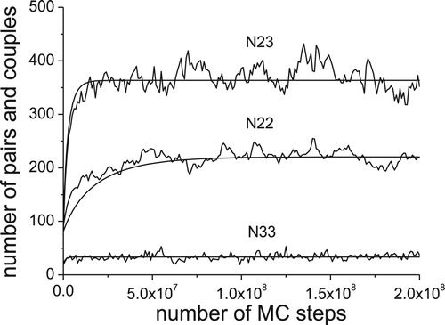
We assume the exchange mechanism between atoms as the diffusion mechanism of solute atoms. This assumption drastically increases the efficiency of the Monte Carlo simulation. Therefore, a rather large system of 1400³ lattice positions can be used for simulations. As the quantities $c_{22}$, $c_{23}$ and $c_{33}$ are directly related to the numbers of pairs and couples $N_{22}$, $N_{23}$ and $N_{33}$ provided by the Monte Carlo simulation, the comparison between the Monte Carlo simulation and the simulation based on the present model is possible. The results are shown in Figure 2 and can be considered as fully satisfactory.

Figure 2. Comparison between the results of Monte Carlo simulation (serrated lines) with simulation based on the present thermodynamic model (smooth lines).

6. Application of the model to an Al-Mg-Si-Cu system

For the demonstration of Cs and Ps formation kinetics let us consider an Al-1Mg-0.8Si-0.4Cu (in at. %) fcc solid solution, i.e. $y_2=0.01$, $y_3=0.008$ and $y_4=0.004$, where Al, Mg, Si and Cu are denoted as components 1, 2, 3 and 4, respectively. The bond formation energies calculated by ab initio are in J/mol units $E_{22}=$−4593, $E_{23}=$−2399, $E_{24}=$−1439, $E_{33}=$−2643, $E_{34}=$−3533, $E_{44}=$−15046.

The tracer diffusion coefficients of the solutes in Al are in m²/s units $D_2=1.49\cdot 10^{-5}\mathrm{e}\mathrm{x}\mathrm{p}\left(120.5\mathrm{k}\mathrm{J}/\mathrm{m}\mathrm{o}\mathrm{l}/\left(R_{g}T\right)\right)$, $D_3=1.38\cdot 10^{-5}\mathrm{e}\mathrm{x}\mathrm{p}\left(117.6\mathrm{k}\mathrm{J}/\mathrm{m}\mathrm{o}\mathrm{l}/\right(R_{g}T\left)\right)$, $D_4=4.44\cdot 10^{-5}\mathrm{e}\mathrm{x}\mathrm{p}\left(133.9\mathrm{k}\mathrm{J}/\mathrm{m}\mathrm{o}\mathrm{l}/\left(R_{g}T\right)\right)$, see Table 3 in [44]. The diffusion coefficients are similar to those published earlier in [45] and can be significantly increased by frozen excess vacancies, see [38]. 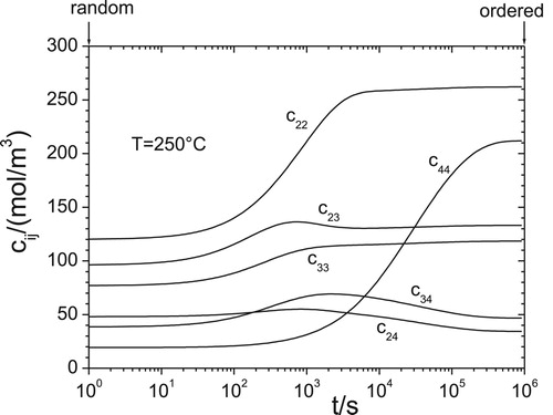$Z=12$ for an fcc lattice. The simulation, presented in Figure 3, starts with the atomic arrangement corresponding to the regular (random) solution model by using $c_{ij}=Z{y}_i{y}_j/\mathrm{\Omega }$, see e.g. [19], and is performed by numerical integration in time of Equations (27, 28), utilising Equations (1–3,8,9) and Equation (22). As a check, the alloy remains random for all $E_{ij}=0$. The simulation, presented in Figure 3, finishes with significantly different values of $c_{ij}$ corresponding to the equilibrium configuration due to the short-range ordering dependent on $E_{ij}$.

Figure 3. Simulation of short-range ordering kinetics in Al-1Mg-0.8Si-0.4Cu solid solution starting as random alloy at 250°C.

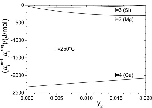
To demonstrate the difference between both concepts, the chemical potentials ${\mu }_i^{\mathrm{r}\mathrm{e}\mathrm{g}}$ from the regular solution model and ${\mu }_i^{\mathrm{o}\mathrm{r}\mathrm{d}}$ from the current short-range ordering model are shown in Figure 4. As already expected the chemical potentials ${\mu }_i^{\mathrm{o}\mathrm{r}\mathrm{d}}$ are lower than ${\mu }_i^{\mathrm{r}\mathrm{e}\mathrm{g}}$. For the determination of equilibrium values of $c_{ij}$ the outlined kinetic procedure, see Equations (27,28), is utilised. The derivatives $\mathrm{\partial }G/\mathrm{\partial }{y}_i$ are evaluated numerically.

Figure 4. Comparison of chemical potentials ${\mu }_i^{\mathrm{o}\mathrm{r}\mathrm{d}}$ (current short-range ordering model) with ${\mu }_i^{\mathrm{r}\mathrm{e}\mathrm{g}}$ (regular solution model) for an Al-1Mg-0.8Si-0.4 Cu solid solution.

7. Discussion

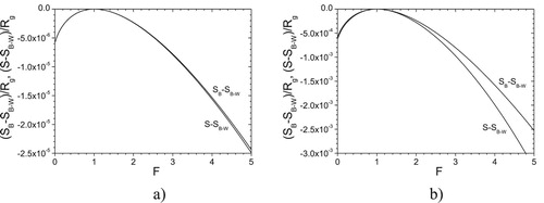
Concerning the formulation of configurational entropy several advanced concepts exist as Cluster Variation Method, introduced by Kikuchi [46] and the computationally much more efficient Cluster-site Approximation Model [47], for details see, e.g. Zhang et al [48]. For the last developments of the Cluster Variation Method, we refer to [49–51]. However, in our case, we have utilised the possibility to divide the system into subsystems with energetically equivalent lattice positions. In this case, the rather classical Bragg–Williams approximation [17] provides an optimal match to the actual situation and, thus, it is used in the present model. Particularly of interest may be a comparison of the present model with Bethe's approximation for binary systems ($n=2$), see [46], Sect. B for details, which is also applicable for non-dilute systems. This allows a comparison with Bethe's approximation, see e.g. [23], estimating to which ‘dilute limit’ the current model is applicable.

For the binary system, the fraction $Y$ of the of solute pairs is given by(29) $Y=c_{22}\mathrm{\Omega }/Z.$(29) Then Bethe’s approximation yields for the configurational entropy(30) $S_{\mathrm{B}}=R_g\left\{\begin{array}{c}\left(Z-1\right)\left[y_2\ln y_2+\left(1-y_2\right)\ln \left(1-y_2\right)\right]-\\ Z\left[Y\ln Y+2\left(y_2-Y\right)\ln \left(y_2-Y\right)+\left(1+Y-2y_2\right)\ln \left(1+Y-2y_2\right)\right]/2\end{array}\right\}.$(30)

$S_{\mathrm{B}}$ can be now compared with the entropy $S$ given by Equations (1–3,8,9,12) as(31) $S=-\frac{R_g}{2}\left[\begin{array}{c}{y}_2\ln y_2+\left(1-y_2\right)\ln \left(1-y_2\right)\\ +N_1\left(y_{12}\ln y_{12}+\left(1-y_{12}\right)\ln \left(1-y_{12}\right)\right)\\ +N_2\left(y_{22}\ln y_{22}+\left(1-y_{22}\right)\ln \left(1-y_{22}\right)\right)\end{array}\right]$(31) with(32) $y_{12}=\left(y_2-c_{22}\mathrm{\Omega }\right)/N_1,y_{22}=c_{22}\mathrm{\Omega }/N_2,N_1=1-Z{y}_2,N_2=Z{y}_2.$(32) Moreover, the Bragg–Williams approximation for the configurational entropy of the system follows as(33) $S_{\mathrm{B}\text{-}\mathrm{W}}=-R_g\left[y_2\ln y_2+\left(1-y_2\right)\ln \left(1-y_2\right)\right].$(33)

The values of $S_{\mathrm{B}}$, $S$ and $S_{\mathrm{B}\text{-}\mathrm{W}}$ should be (and they really are) identical for an ideal (random) solution, i.e. for the value $c_{22}=Z{y}_2^2/\mathrm{\Omega }$. To compare our approach with Bethe’s approximation, we vary $c_{22}$ by a multiplier $F$ as $c_{22}=FZ{y}_2^2/\mathrm{\Omega }$ and plot the dependences $S_{\mathrm{B}}-S_{\mathrm{B}\text{-}\mathrm{W}}$ and $S-S_{\mathrm{B}\text{-}\mathrm{W}}$ versus $F$. Note that $S_{\mathrm{B}\text{-}\mathrm{W}}$ is independent of $F$. For a rather dilute solution with $y_2=0.001$ the functions $S_{\mathrm{B}}\left(F\right)$ and $S\left(F\right)$ practically coincide (see Figure 5(a)). Also for $y_2=0.01$ their agreement is still satisfactory (see Figure 5(b)). Consequently one can expect that the current model is applicable to solute site fractions up to about 1%. This can be even more than 1% for repulsive interactions or weakly attractive interactions, see Figure 5(b).

Figure 5. Comparison of configurational entropy of a binary system calculated by Bethe's approximation $S_{\mathrm{B}}$ and by the current model $S$ for (a) $y_2=0.001$ and (b) $y_2=0.01$.

As a further comparison, we investigate the (negative) driving force $\mathrm{\partial }G/\mathrm{\partial }{c}_{22}$. The only difference between the driving forces calculated for the current model and Bethe’s approximation [41] lies in the different entropy terms $S$ and $S_{\mathrm{B}}$, resp. Using Equations (29) and (30), we find the following difference(34) $T\frac{\mathrm{\partial }\left(S_B-S\right)}{\mathrm{\partial }{c}_{22}}=\frac{\mathrm{\Omega }}{2}{R}_{g}T\ln \left[\frac{1-y_{22}}{1-Z{y}_{22}}\frac{\left(1-y_2\right)-Z{y}_2\left(1-y_{22}\right)}{\left(1-y_2\right)-y_2\left(1-y_{22}\right)}\right].$(34) This relation has been found after some algebra using Equation (8) together with Equation (2), yielding $c_{22}\mathrm{\Omega }=y_{22}{N}_2=y_{22}{y}_{2}Z$. It should be noted that the above difference disappears for $Z=1$ and includes only $y_2$ and $y_{22}$. To utilise Bethe’s approximation, the above term (34) has to be added to the $\mathrm{\partial }G/\mathrm{\partial }{c}_{22}$ in the current binary model.

Finally, we would like to point to our assumption of a dilute solution, which is consistent with the assumption that the prevailing solute – solute bonds exist in Cs and Ps. Only in that case, the application of the bond formation energies $E_{ij}$ determined by ab initio calculations is justified and, moreover, in the dilute case, the number of bonds in clusters of more than two solute atoms is negligible. The applicability of our concept to multicomponent systems as well as treatment of its kinetics can be considered as an important novelty.

8. Conclusions

The regular solution model is established for the treatment of disordered alloys. This model assumes that the interaction energies between nearest atoms are known and the atoms are randomly arranged in the lattice. Thus the concentrations of the bonds between individual solute atoms are independent of the values of the interaction energies. According to random state is then considered as the equilibrium state.

In reality, however, the interaction energies influence the concentrations of the bonds between individual solute atoms. The concentrations can be considered as internal state variables and so describe the short-range ordering in the solid solution. The Gibbs energy of the initially random system decreases due to short-range ordering and tends towards its minimum. The current original short-range ordering model allows evaluation of

• the Gibbs energy of a dilute multicomponent system as a function of Cs and Ps concentrations and corresponding formation energies of the bonds between individual solute atoms,

• the evolution of the multicomponent system via the kinetics of the concentrations of Cs and Ps, controlled by diffusion of individual components,

• the equilibrium state by time integration of the evolution equations until the stationary state is reached,

• thermodynamic potentials of the solid solution in equilibrium.

These achievements can be considered as substantial progress in the field of non-equilibriun and equilibrium thermodynamics of solid solutions.

The current short-range ordering model is checked by comparison with the Monte Carlo simulation and demonstrated for the Al-Mg-Si-Cu system. The bond formation energies are determined by ab initio calculations. The diffusion coefficients of the solutes are taken from the literature. The kinetics of short-range ordering in an initially random system tending to equilibrium is simulated. The chemical potentials of solutes are calculated for the current short-range ordering and the established regular solution models and exhibit remarkable differences between them.

Finally, it shall be mentioned that the current concept can be extended to further energy terms if an interaction of the energetics of those processes with the chemical process takes place. Here we refer to magnetic exchange transactions as dealt with by Korzhavyi et al. [52]. Any atomistic misfit can also be included in this concept taking into account the mechanical interaction energy. Furthermore, the role of vacancies can be included in the chemical process. With respect to the interactions with pressure and vacancies, we refer to two of our previous papers [43,53].

Acknowledgements

The authors express their thanks to R. Kozubski (Jagiellonian University, Krakow, Poland) for helpful discussions. The computational results presented have been achieved using the Vienna Scientific Cluster (VSC).

Disclosure statement

No potential conflict of interest was reported by the authors.

Additional information

Funding

Financial support was provided by the Austrian Federal Government (in particular from the Bundesministerium für Verkehr, Innovation and Technologie and the Bundesministerium für Wirtschaft und Arbeit) and the Styrian Provincial Government, represented by Österreichische Forschungsförderungsgesellschaft mbH and by Steirische Wirtschaftsförderungsgesellschaft mbH, within the research activities of the K2 Competence Centre on ‘Integrated Research in Materials, Processing and Product Engineering’, operated by the Materials Center Leoben Forschung GmbH in the framework of the Austrian COMET Competence Centre Programme, Projects A1.23, is gratefully acknowledged. J.S. gratefully acknowledges the financial support provided by the Ministry of Education and Sports of the Czech Republic within the research project ‘Architectured materials designed for additive manufacturing’, Reg. No.: CZ.02.1.01/0.0/0.0/16_025/0007304.

References

- G. Yuan, M. Liu, W. Ding and A. Inoue, Mechanical properties and microstructure of Mg-Al-Zn-Si-base alloy. Mater. Trans. 44 (2003), pp. 458–462. doi: 10.2320/matertrans.44.2271
- M. Wang, Y. Xu, Q. Zheng, S. Wu, T. Jing and N. Chawla, Dendritic growth in Mg-based alloys: Phase-field simulations and experimental verification by X-ray synchrotron tomography. Metall. Mater. Trans. A 45 (2014), pp. 2562–2574. doi: 10.1007/s11661-014-2200-x
- C. Kammer, Aluminium Handbook: Fundamentals and Materials, Vol. 1, Beuth, Berlin, 2011.
- S. Pogatscher, H. Antrekowitsch, M. Werinos, F. Moszner, S.S.A. Gerstl, M.F. Francis, W.A. Curtin, J.F. Löffler and P.J. Ugowitzer, Diffusion on demand to control precipitation aging: application to Al-Mg-Si alloys. Phys. Rev. Letters 112 (2014), p. 225701 (p. 5). doi: 10.1103/PhysRevLett.112.225701
- D.J. Chakrabarti and D.E. Loughlin, Phase relations and precipitation in Al–Mg–Si alloys with Cu additions. Prog. Mater. Sci 49 (2004), pp. 389–410. doi: 10.1016/S0079-6425(03)00031-8
- J. Temple Black and R.A. Kohser, Degarmo’s Materials and Processes in Manufacturing, 10th ed., Wiley, Hoboken, 2007.
- B.C. DeCooman and J.G. Speer, Fundamentals of Steel Product Physical Metallurgy, AIST, Warrendall, PA, 2012.
- I.V. Masanskii, V.I. Tokar and T.A. Grishenko, Pair interactions in alloys evaluated from diffuse-scattering data. Phys. Rev. B 44 (1991), pp. 4647–4649. doi: 10.1103/PhysRevB.44.4647
- P.C. Clapp and S.C. Moss, Correlation functions of disordered binary alloys. I. Phys. Rev. 142 (1966), pp. 418–427. doi: 10.1103/PhysRev.142.418
- P.C. Clapp and S.C. Moss, Correlation functions of disordered binary alloys. II. Phys. Rev. 171 (1968), pp. 754–763. doi: 10.1103/PhysRev.171.754
- S.C. Moss and P.C. Clapp, Correlation functions of disordered binary alloys. III. Phys. Rev. 171 (1968), pp. 764–777. doi: 10.1103/PhysRev.171.764
- M.A. Krivoglaz, Theory of X-ray and Thermal-neutron Scattering by Real Crystals, Plenum Press, New York, 1969.
- J. Banhart, M.D.H. Lay, C.S.T. Chang and A.J. Hill, Kinetics of natural aging in Al-Mg-Si alloys studied by positron annihilation liftetime spectroscopy. Phys. Rev. B 83 (2011), p. 014101 (p. 13). doi: 10.1103/PhysRevB.83.014101
- H.L. Lukas, S.G. Fries and B. Sundman, Computational Thermodynamics, the Calphad Method, Cambridge University Press, Cambridge, 2007.
- P. Mason, Thermo-Calc software; software available at www.thermocalc.com
- [16] E. Kozeschnik, MatCalc 6, the materials calculator; software available at www.matcalc.tuwien.ac.at
- W.L. Bragg and E.J. Williams, The effect of thermal agitation on atomic arrangement in alloy. Proc. Roy. Soc. Lond. 145A (1934), pp. 699–730 and 151A (1935), pp. 540–566.
- J. Svoboda, Y.V. Shan and F.D. Fischer, A new self-consistent model for thermodynamics of binary solutions. Scripta Mater. 108 (2015), pp. 27–30. doi: 10.1016/j.scriptamat.2015.06.014
- J. Svoboda and F.D. Fischer, A self-consistent model for thermodynamics of multicomponent solid solutions. Scripta Mater. 123 (2016), pp. 154–157. doi: 10.1016/j.scriptamat.2016.05.024
- V.A. Shabashov, K.A. Kozlov, V.V. Sagaradze, A.L. Nikolaev, K.A. Lyashkov, V.A. Semyonkin and V.I. Voronin, Short-range order clustering in BCC Fe-Mn alloys induced by severe plastic deformation. Philos. Mag. 98 (2018), pp. 560–576. doi: 10.1080/14786435.2017.1412586
- M.L. Kapoor, Interpretation of the thermodynamics of metallic solutions by lattice models. Int. Metall. Rev. 20 (1975), pp. 150–165. doi: 10.1179/imr.1975.20.1.150
- R.H. Fowler, A modernized version of Gibbs’ use of the grand canonical ensemble. Math. Proc. Camb. Philos. Soc. 34 (1938), pp. 382–391. doi: 10.1017/S0305004100020326
- H.A. Bethe and H. Wills, Statistical theory of superlattices. Proc. Roy. Soc. 150A (1935), pp. 552–575.
- E.A. Guggenheim, The statistical mechanics of regular solutions. Proc. Royal Soc. A148(864) (1935), pp. 304–312.
- G.S. Rushbrooke, A note on Guggenheims theory of strictly regular binary liquid mixtures. Proc. Royal Soc. A166(925) (1938), pp. 296–315.
- C.H.P. Lupis and J.F. Elliott, Prediction of enthalpy and entropy interaction coefficients by the ‘central atoms’ theory. Acta Metall. 15 (1967), pp. 265–276. doi: 10.1016/0001-6160(67)90202-7
- J.-C. Mathieu, F. Durand and E. Bonnier, L'atome entouré, entité de base d'un modéle quasichimique de solution binaire – I. – Traitement général. J. Chim. Phys. 62 (1965), pp. 1289–1296. doi: 10.1051/jcp/1965621289
- J.-C. Mathieu, F. Durand and E. Bonnier, L'atome entouré, entité de based'un modéle quasichimique de solution binaire – II. – Influence de deux formes d'energie potentielle sur l'enthalpie de mélange. J. Chim. Phys. 62 (1965), pp. 1297–1303. doi: 10.1051/jcp/1965621297
- M. Hillert, The compound energy formalism. J. Alloys Compd. 320 (2001), pp. 161–176. doi: 10.1016/S0925-8388(00)01481-X
- V.A. Shabashov, K.A. Kozlov, A.L. Nikolaev, A.E. Zamatovskii, V.V. Sagaradze, E.G. Novikov and K.A. Lyashkov, The short-range clustering in Fe-Cr alloys enhanced by severe plastic deformation and electron irradiation. Philos. Mag. 100 (2020), pp. 1–17. doi: 10.1080/14786435.2019.1660012
- Y.J. Zhang, D. Han and X.W. Li, A unique two-stage strength-ductility match in low solid-solution hardening Ni-Cr alloys: decisive role of short range ordering. Scripta Mater. 178 (2020), pp. 269–273. doi: 10.1016/j.scriptamat.2019.11.049
- G. Kresse and J. Furthmüller, Efficient iterative schemes for ab initio total-energy calculations using a plane-wave basis set. Phys. Rev. B 54 (1996), pp. 11169–11186. doi: 10.1103/PhysRevB.54.11169
- G. Kresse and D. Joubert, From ultrasoft pseudopotentials to the projector augmented-wave method. Phys. Rev. B 59 (1999), pp. 1758–1775. doi: 10.1103/PhysRevB.59.1758
- J.P. Perdew, K. Burke and M. Ernzerhof, Generalized gradient approximation made simple. Phys. Rev. Lett. 77 (1996), pp. 3865–3868. doi: 10.1103/PhysRevLett.77.3865
- P. Haas, F. Tran and P. Blaha, Calculation of the lattice constant of solids with semilocal functionals. Phys. Rev. B 79 (2009), p. 085104. (p. 10). doi: 10.1103/PhysRevB.79.085104
- O.I. Gorbatov, A. Yu Stroev, Y.N. Gornostyrev and P.A. Korzhavyi, Effective cluster interactions and pre-precipitate morphology in binary Al-based alloys. Acta Mater. 179 (2019), pp. 70–84. doi: 10.1016/j.actamat.2019.08.011
- J. Svoboda, F.D. Fischer, P. Fratzl and A. Kroupa, Diffusion in multi-component systems with no or dense sources and sinks for vacancies. Acta Mater. 50 (2002), pp. 1369–1381. doi: 10.1016/S1359-6454(01)00443-8
- J. Svoboda, Y.V. Shan, E. Kozeschnik and F.D. Fischer, A thermokinetic model for Mg-Si couple formation in Al-Mg-Si alloys. Modell. Simul. Mater. Sci. Eng. 24 (2016), p. 035021. (p. 15). doi: 10.1088/0965-0393/24/3/035021
- F.D. Fischer, J. Svoboda and H. Petryk, Thermodynamic extremal principles for irreversible processes in materials science. Acta Mater. 67 (2014), pp. 1–20. doi: 10.1016/j.actamat.2013.11.050
- J. Svoboda, Y.V. Shan, E. Kozeschnik and F.D. Fischer, Couples and pairs formation – thermodynamic and kinetic modelling applied to Al-Mg-Si. Modell. Simul. Mater. Sci. Eng. 25 (2017), p. 065011. (p. 15). doi: 10.1088/1361-651X/aa76cf
- N. Metropolis, A.W. Rosenbluth, M.N. Rosenbluth, A.H. Teller and E. Teller, Equation of state calculations by fast computing machines. J. Chem. Phys. 21 (1953), pp. 1087–1092. doi: 10.1063/1.1699114
- C. Bichara and G. Inden, Gibbs energies and chemical potentials of solid solution phases. Prog. Theor. Phys. Supplement 115 (1994), pp. 171–184. doi: 10.1143/PTPS.115.171
- J. Svoboda and F.D. Fischer, Diffusion of elements and vacancies in multi-component systems. Prog. Mater. Sci. 60 (2014), pp. 338–367. doi: 10.1016/j.pmatsci.2013.09.001
- Y. Du, Y.A. Chang, B. Huang, W. Gong, Z. Jin, H. Xu, Z. Yuan, Y. Liu, Y. He and F.-Y. Xie, Diffusion coefficients of some solutes in fcc and liquid Al: critical evaluation and correlation. Mater. Sci. Eng. A 363 (2003), pp. 140–151. doi: 10.1016/S0921-5093(03)00624-5
- X. Yan, S. Chen, F. Xie and Y.A. Chang, Computational and experimental investigation of microsegregation in an Al-rich Al-Cu-Mg-Si quaternary alloy. Acta Mater. 50 (2002), pp. 2199–2207. doi: 10.1016/S1359-6454(01)00431-1
- R. Kikuchi, A theory cooperative phenomena. Phys. Rev. 81 (1951), pp. 988–1003. doi: 10.1103/PhysRev.81.988
- Y.-Y. Li, Quasi-chemical method in statistical theory of regular mixtures. Phys. Rev. 76 (1949), pp. 972–979. doi: 10.1103/PhysRev.76.972
- F. Zhang, Y.A. Chang, Y. Du, S.-L. Chan and W.A. Oates, Application of cluster-site approximation (CSA) model to the f.c.c. phase in the Ni-Al system. Acta Mater. 51 (2003), pp. 207–216. doi: 10.1016/S1359-6454(02)00392-0
- N. Kiyokane and T. Mohri, Modelling of a displacive transformation in two-dimensional system within a single-site approximation of continuous displacement cluster variation method. Philos. Mag. 93 (2013), pp. 2316–2328. doi: 10.1080/14786435.2013.770611
- N. Kiyokane and T. Mohri, Modelling of a displacive transformation in two-dimensional system with four-body approximation of continuous displacement cluster variation method. Philos. Mag. 98 (2018), pp. 1005–1017. doi: 10.1080/14786435.2018.1433885
- N. Bourgeois, P. Cenedese, J.-C. Crivello and J.-M. Joubert, Pd-H and Ni-H phase diagrams using cluster variation method and Monte Carlo simulation. Philos. Mag. 99 (2019), pp. 2376–2392. doi: 10.1080/14786435.2019.1628367
- P.A. Korzhavyi, A.V. Ruban, J. Odqvist, J.-O. Nilsson and B. Johansson, Electronic structure and effective chemical and magnetic exchange interactions in bcc Fe-Cr alloys. Phys. Rev. B 79 (2009), 054202-1-16. doi: 10.1103/PhysRevB.79.054202
- J. Svoboda, F.D. Fischer and P. Fratzl, Diffusion and creep in multi-component alloys with non-ideal sources and sinks for vacancies. Acta Mater. 54 (2006), pp. 3043–3053. doi: 10.1016/j.actamat.2006.02.041