Laguerre tessellations and polycrystalline microstructures: a fast algorithm for generating grains of given volumes

ABSTRACT

We present a fast algorithm for generating Laguerre diagrams with cells of given volumes, which can be used for creating RVEs of polycrystalline materials for computational homogenisation, or for fitting Laguerre diagrams to EBSD or XRD measurements of metals. Given a list of desired cell volumes, we solve a convex optimisation problem to find a Laguerre diagram with cells of these volumes, up to any prescribed tolerance. The algorithm is built on tools from computational geometry and optimal transport theory which, as far as we are aware, have not been applied to microstructure modelling before. We illustrate the speed and accuracy of the algorithm by generating RVEs with user-defined volume distributions with up to 20,000 grains in 3D. We can achieve volume percentage errors of less than 1% in the order of minutes on a standard desktop PC. We also give examples of polydisperse microstructures with bands, clusters and size gradients, and of fitting a Laguerre diagram to 3D EBSD measurements of an IF steel.

KEYWORDS:

• Laguerre diagrams
• power diagrams
• polycrystalline materials
• grains
• foams
• volume distribution

1. Introduction

1.1. State of the art

Voronoi diagrams and their generalisations are often used to represent the microstructure of polycrystalline metals and foams, e.g. [1–14], with individual Voronoi cells representing grains in metals and pores or bubbles in foams. They can be used to generate complex microstructures quickly using a relatively small number of parameters, and they are often used as representative volume elements (RVEs) for computational homogenisation, e.g. [15–17].

In this paper, we focus on the class of weighted Voronoi diagrams known as Laguerre diagrams (or power diagrams or radical Voronoi tessellations), which provide a more accurate description of the geometry of polycrystalline materials than classical Voronoi diagrams [8,14]. However, Laguerre diagrams share the limitation of Voronoi diagrams that there is not an explicit relation between their generators and their geometric properties, such as the volumes of their cells. Consequently, an active area of research is to develop algorithms for generating Laguerre diagrams with prescribed geometric properties.

One popular method for approximately controlling the grain size distribution of Laguerre diagrams is using random close packing of spheres and ellipsoids [4,8,10,18]. This method is inexact, however, since it is impossible to tessellate Euclidean space with spheres or ellipsoids.

Several authors have developed methods for fitting Laguerre diagrams to image data (EBSD, XRD) of polycrystals. Here, geometric properties such as grain size, centroid location, and aspect ratio are fitted by minimising a measure of the fitting error using deterministic and stochastic optimisation methods, e.g. [3,9,11,19,20]. While optimisation methods can give very accurate results, they can also be computationally expensive. Heuristic methods such as [13] trade-off fidelity against speed.

Recently, several authors have generated RVEs with curved boundaries and non-convex cells grains using generalisations of Laguerre diagrams such as generalised balanced power diagrams [1,12,13,21] and multilevel Voronoi diagrams [5,17]. Complex geometries can also be created using the open-source software DREAM.3D [22] and Neper [23].

We will discuss some of these methods in more detail and compare them with ours in the Discussion section.

1.2. Goal of this paper

The goal of this paper is to develop algorithms for creating Laguerre diagrams with user-defined cell size distributions. Our motivation comes from steel modelling. We wish to generate realistic RVEs of single- and multi-phase steels for computational homogenisation simulations. Unlike much of the literature on Laguerre modelling of polycrystals [1,12,13,24], our primary aim is not to fit Laguerre diagrams to EBSD or XRD data, but rather to create a tool for generating a rich family of (possibly never-observed) microstructures, which can be combined with multiscale simulations to optimise grain geometries and lead to the development of new alloys. Having said that, our algorithms are also very well suited for generating Laguerre diagrams with texture intensities that match EBSD data, as we demonstrate in Example 5.3. With these applications to steel in mind, we often refer to Laguerre cells as grains, although our results can be applied more generally to other polycrystalline metals and to foams.

1.3. Contributions and outline of the paper

In Section 2, we recall the definition and some important properties of Laguerre diagrams. In particular, Property 2.3 forms the basis of our work. Section 3 includes our main result, Algorithm 2, for generating ‘regularised’ Laguerre diagrams with grains of prescribed volumes, up to any given tolerance. We also provide Algorithm 1 that can be used for fitting a Laguerre diagram to EBSD measurements of grain volumes and centroids (Example 5.3). We discuss practical issues about how the algorithms can be implemented in Section 4. Section 5 includes some large examples (10,000+ grains) and run-time tests in 3D, including examples of RVEs of Interstitial Free (IF) steels.

The theory underlying the algorithms presented in Section 2 uses results from computational geometry and optimal transport theory [25,26], a field of mathematics that has recently enormously grown in importance and found applications in a wide range of areas including data science, economics, image processing, partial differential equations and statistics. We believe however that this is its first application in the steel industry.

2. Laguerre diagrams

2.1. Notation and definitions

Let $\mathrm{\Omega }\subset {\mathbb{R}}^d$ be the region occupied by a metal. We consider both the 2- and 3-dimensional cases ($d=2$ and $d=3$). For simplicity, we assume that $\mathrm{\Omega }$ is a convex polygon if $d=2$ or a convex polyhedron if $d=3$. In principle, the algorithms below can be used for non-convex regions with curved boundaries, but they become harder to implement. In all our examples below, we take $\mathrm{\Omega }$ to be a rectangular box. If $U$ is a subset of $\mathrm{\Omega }$, let $\left|U\right|$ denote its area if $d=2$ or its volume if $d=3$.

Definition 2.1

([27], [28]):

Let $x_1,\dots ,x_n$ be distinct points in $\mathrm{\Omega }$ and $w_1,\dots ,w_n$ be real numbers (not necessarily positive). The Laguerre diagram or power diagram generated by the weighted points $(x_1,w_1),\dots ,(x_n,w_n)$ is the tessellation $\{L_i{\}}_{i=1}^n$ of $\mathrm{\Omega }$ defined by(1) $L_i=\left\{x\in \mathrm{\Omega }:|x-x_i{|}^2-w_i\le |x-x_j{|}^2-w_j\mathrm{\forall }j\in \{1,\dots ,n\}\right\}.$(1) We refer to the sets $L_i$ as Laguerre cells or grains.

Laguerre diagrams have the following basic properties [27,28]:

• Laguerre cells are convex polygons if $d=2$ or convex polyhedra if $d=3$.

• The Laguerre cells tessellate $\mathrm{\Omega }$, which means that $\bigcup _{i=1}^n{L}_i=\mathrm{\Omega }$ and cells can only intersect along their boundaries.

• If all the weights are equal, $w_1=w_2=\cdots =w_n$, then the Laguerre diagram is simply a Voronoi diagram.

• Adding a constant to all the weights does not affect the Laguerre diagram, i.e. the weighted points $\left\{\right(x_i,w_i){\}}_{i=1}^n$ and $\left\{\right(x_i,w_i+c){\}}_{i=1}^n$ generate the same diagram for any $c\in \mathbb{R}$.

• A generator $x_i$ needs not belong to its Laguerre cell $L_i$.

• There can be empty Laguerre cells, $L_j=\mathrm{\varnothing }$ for some $j$.

Now, we recall two advanced properties of Laguerre diagrams, Properties 2.2 and 2.3. These are the key ingredients for generating RVEs with grains of given sizes (given areas if $d=2$ or given volumes if $d=3$). Property 2.2 states that there always exists a Laguerre diagram with grains of given sizes. Property 2.3 gives a constructive way of finding one.

Property 2.2

([27, p. 96, Corollary 6.1], [29]):

Let $x_1,\dots ,x_n$ be distinct points in $\mathrm{\Omega }$. Let $m_1,\dots ,m_n$ be positive numbers with $\sum _{i=1}^n{m}_i=\left|\mathrm{\Omega }\right|$. Then there exist weights $w_1,\dots ,w_n$ such that the Laguerre diagram $\{L_i{\}}_{i=1}^N$ generated by $(x_1,w_1),\dots ,(x_n,w_n)$ has cells of size $m_1,\dots ,m_n$:(2) $\left|L_i\right|=m_i\mathrm{f}\mathrm{o}\mathrm{r}\mathrm{a}\mathrm{l}\mathrm{l}i\in \{1,\dots ,n\}.$(2)

The weights $w_i$ in Property 2.2 can be computed using the following result.

Property 2.3

([27, pp. 98–100], [29], [30, Theorem 2]):

Let $x_1,\dots ,x_n$ be distinct points in $\mathrm{\Omega }$. Let $m_1,\dots ,m_n$ be positive numbers with $\sum _{i=1}^n{m}_i=\left|\mathrm{\Omega }\right|$. Define the function $g:{\mathbb{R}}^n\to \mathbb{R}$ by(3) $g(w_1,\dots ,w_n)=\sum _{i=1}^n(m_i-|L_i\left|\right)w_i+\sum _{i=1}^n{\int }_{L_i}|x-x_i{|}^2\mathrm{d}x,$(3) where $\{L_i{\}}_{i=1}^N$ is the Laguerre diagram generated by $(x_1,w_1),\dots ,(x_n,w_n)$. Then

1. The function $g$ is concave.

2. The gradient of $g$ has components(4) $\frac{\mathrm{\partial }g}{\mathrm{\partial }{w}_i}=m_i-\left|L_i\right|$(4) for all $i\in \{1,\dots ,n\}$.

3. If $w=(w_1,\dots ,w_n)$ is a critical point of $g$, i.e. if $\mathrm{\nabla }g\left(w\right)=0,$ then the Laguerre diagram $\{L_i{\}}_{i=1}^N$ generated by $(x_1,w_1),\dots ,(x_n,w_n)$ has cells of size $m_1,\dots ,m_n:$(5) $\left|L_i\right|=m_i\mathrm{f}\mathrm{o}\mathrm{r}\mathrm{a}\mathrm{l}\mathrm{l}i\in \{1,\dots ,n\}.$(5)

Property 2.3 forms the basis of Algorithms 1 and 2. It means that if we want to generate a Laguerre diagram with grains of given sizes, then we just need to find critical points of $g$. Since $g$ is concave, this is equivalent to maximising $g$, or to minimising $-g$, which is a smooth, unconstrained, convex optimisation problem. Fast numerical methods are available for solving this [31].

2.2. Controlling the spatial distribution of grains

Property 2.3 not only allows one to control the size distribution of grains, it also gives some control over the spatial distribution. Given positive numbers $m_1,\dots ,m_n$ with $\sum _{i=1}^n{m}_i=\left|\mathrm{\Omega }\right|$, there are infinitely many Laguerre diagrams $\{L_i{\}}_{i=1}^n$ such that $\left|L_i\right|=m_i$ for all $i\in \{1,\dots ,n\}$. This can be seen from Property 2.3(iii); any choice of distinct points $x_1,\dots ,x_n$ can give a Laguerre diagram with grains of size $m_1,\dots ,m_n$. In Section 4.3.1, we will show how to choose $x_1,\dots ,x_n$ to control the spatial distribution of the grains.

2.3. Connection with optimal transport theory

Properties 2.2 and 2.3 can also be stated in the language of semi-discrete optimal transport theory¹; see, e.g. [26, Sec. 6.4.2], [30], [32]. This connection provides a way of finding critical points of $g$ using fast modern methods from optimal transport theory [32,33]. We discuss this connection further at the end of Section 3.2.3.

3. Main results

3.1. Statement of the algorithms

For concreteness we state the algorithms in three dimensions, but they can also be used in two dimensions (by substituting volume with area and polyhedron with polygon wherever they appear in Algorithms 1 and 2). Our main result is Algorithm 2. First, however, we consider a simplified version, Algorithm 1, which will help us to understand the importance of the regularisation step in Algorithm 2. Algorithm 1 can also be used for data-driven modelling to fit a Laguerre diagram to EBSD or XRD measurements of grain volumes and centroids (see Example 5.3). Algorithm 1 is not new and goes back at least as far as [29]. Our role is simply to bring it to the attention of the microstructure modelling community.

Algorithm 1: Generate a Laguerre diagram with grains of given volumes.

Input: A convex polyhedron $\mathrm{\Omega }$ representing a sample of metal, a list of volumes $m_1,\dots ,m_n$ such that $m_i>0$ and $\sum _{i=1}^n{m}_i=\left|\mathrm{\Omega }\right|$, and a relative error tolerance $\epsilon$.

Output: The generators $(x_1,w_1),\dots ,(x_n,w_n)$ of a Laguerre diagram $\{L_i{\}}_{i=1}^n$ such that grain $L_i$ has volume $m_i$ up to $\epsilon$ relative error, i.e. $\frac{\parallel L_i|-m_i|}{m_i}<\epsilon$, for all $i\in \{1,\dots ,n\}$.

Method:

Initialisation. Choose or randomly select $n$ distinct points $x_1,\dots ,x_n$ in $\mathrm{\Omega }$.

Optimisation step. Use a numerical optimisation method to find $w=(w_1,\dots ,w_n)$ that maximises the function $g$ defined in equation (3(3) $g(w_1,\dots ,w_n)=\sum _{i=1}^n(m_i-|L_i\left|\right)w_i+\sum _{i=1}^n{\int }_{L_i}|x-x_i{|}^2\mathrm{d}x,$(3) ). Initialise the optimisation method using the initial guess $w_{\mathrm{i}\mathrm{n}\mathrm{i}\mathrm{t}}=0$ and terminate it using the stopping criterion $\left|\mathrm{\nabla }g\right(w\left)\right|<\epsilon \underset{j}{min}{m}_j$.

Example 3.1

(Example of Algorithm 1):

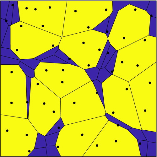
Figure 1 shows an example of Algorithm 1 implemented in MATLAB with $n=50$ grains in the square domain $\mathrm{\Omega }=[0,1]\times [0,1]$. The grains have target areas $m_i=x$ for $i\in \{1,\dots ,35\}$ and $m_i=10x$ for $i\in \{36,\dots ,50\}$, where $x=1/185$ so that the total area of all the grains equals the area of $\mathrm{\Omega }$. The actual areas of the grains returned by Algorithm 1 are correct to within $1\text{\%}$ error ($\epsilon =0.01$). The initialisation step of Algorithm 1 was performed using the MATLAB function rand to select $x_1,\dots ,x_{50}$ (pseudo)randomly from a uniform distribution. While the grains have the correct areas to within $1\text{\%}$, the microstructure is somewhat irregular and unrealistic, with some highly elongated grains. This leads us to Algorithm 2, which produces more regular microstructures; compare Figures 1 and 2(i).

Algorithm 2: Generate a regularised Laguerre diagram with grains of given volumes.

Input: A convex polyhedron $\mathrm{\Omega }$ representing a sample of metal, a list of volumes $m_1,\dots ,m_n$ such that $m_i>0$ and $\sum _{i=1}^n{m}_i=\left|\mathrm{\Omega }\right|$, a relative error tolerance $\epsilon$, and the number of regularisation steps $K$.

Figure 1. An example of Algorithm 1 with $n=50$ grains in the unit square $\mathrm{\Omega }$. There are 35 small grains and 15 large grains. The small grains have area $x$ and the large grains have area $10x$ to within $1\text{\%}$ error, where $x=1/185$. The black dots are the locations of the generators $\{x_i{\}}_{i=1}^{50}$. Notice that not every grain contains its own generator.

Output: The generators $(x_1,w_1),\dots ,(x_n,w_n)$ of a regularised Laguerre diagram $\{L_i{\}}_{i=1}^n$ such that grain $L_i$ has volume $m_i$ up to $\epsilon$ relative error, i.e. $\frac{\parallel L_i|-m_i|}{m_i}<\epsilon$, for all $i\in \{1,\dots ,n\}$.

Method:

Initialisation. Choose or randomly select $n$ distinct points $x_1^{\left(0\right)},\dots ,x_n^{\left(0\right)}$ in $\mathrm{\Omega }$. Initialise the weights to be zero: $w^{\left(0\right)}=(w_1^{\left(0\right)},\dots ,w_n^{\left(0\right)})=0$.

Iteration. For $k=1,\dots ,K$ do:

• (1) Regularisation step. For $i\in \{1,\dots ,n\}$, define $x_i^{\left(k\right)}$ to be the centroid of $L_i^{(k-1)}$: (6) $x_i^{\left(k\right)}:=\frac{1}{|L_i^{(k-1)}|}{\int }_{L_i^{(k-1)}}x\mathrm{d}x,$(6) where $\{L_i^{(k-1)}{\}}_{i=1}^n$ is the Laguerre diagram obtained in the previous iteration, which is generated by $(x_1^{(k-1)},w_1^{(k-1)}),\dots ,(x_n^{(k-1)},w_n^{(k-1)})$.

• (2) Optimisation step. Use a numerical optimisation method to find $w^{\left(k\right)}=(w_1^{\left(k\right)},\dots ,w_n^{\left(k\right)})$ that maximises the concave function(7) $g_k(w_1,\dots ,w_n)=\sum _{i=1}^n(m_i-|L_i|)w_i+\sum _{i=1}^n{\int }_{L_i}|x-x_i^{\left(k\right)}{|}^2\mathrm{d}x,$(7) where $\{L_i{\}}_{i=1}^n$ is the Laguerre diagram generated by $(x_1^{\left(k\right)},w_1),\dots ,(x_n^{\left(k\right)},w_n)$. Initialise the optimisation method using the initial guess $w_{\mathrm{i}\mathrm{n}\mathrm{i}\mathrm{t}}=w^{(k-1)}$ and terminate it using the stopping criterion $|\mathrm{\nabla }{g}_k(w^{\left(k\right)})|<\epsilon \underset{j}{min}{m}_j$.

Return. Output the generators $\{(x_i,w_i){\}}_{i=1}^n=\{(x_i^{\left(K\right)},w_i^{\left(K\right)}){\}}_{i=1}^n$.

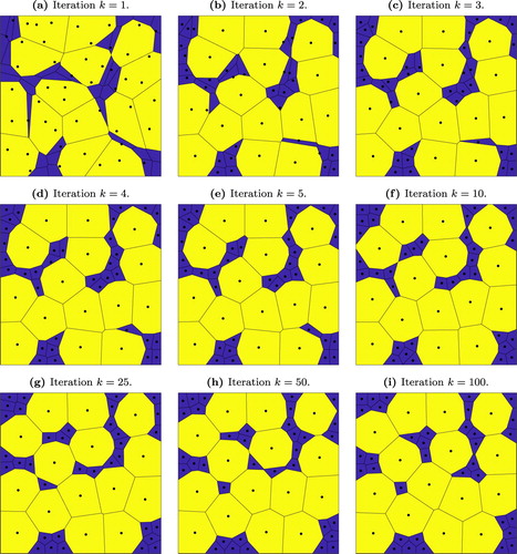
Figure 2. An example of $K=100$ iterations of Algorithm 2 with $n=50$ grains in the unit square $\mathrm{\Omega }$. There are 35 small grains and 15 large grains. The small grains have area $x$ and the large grains have area $10x$ to within $1\text{\%}$ error, where $x=1/185$. The black dots are the locations of the generators $\{x_i{\}}_{i=1}^{50}$. In figure (i), the generators $x_i$ are located at the centroids of their cells $L_i$ to within a distance of 0.002. (a) Iteration $k=1$. (b) Iteration $k=2$. (c) Iteration $k=3$. (d) Iteration $k=4$. (e) Iteration $k=5$. (f) Iteration $k=10$. (g) Iteration $k=25$. (h) Iteration $k=50$. (i) Iteration $k=100$.

Example 3.2

(Example of Algorithm 2):

Figure 2 shows an example of Algorithm 2, using $K=100$ iterations, implemented in MATLAB with $n=50$ grains in the square domain $\mathrm{\Omega }=[0,1]\times [0,1]$. The grains have target areas $m_i=x$ for $i\in \{1,\dots ,35\}$ and $m_i=10x$ for $i\in \{36,\dots ,50\}$, where $x=1/185$ so that the total area of all the grains equals the area of $\mathrm{\Omega }$. The actual areas of the grains returned by Algorithm 2 are correct to within $1\text{\%}$ error ($\epsilon =0.01$). For the initialisation step we used exactly the same points $x_1^{\left(0\right)},\dots ,x_n^{\left(0\right)}$ that were used for the initialisation step in Example 3.1. Observe from Figure 2 how the Laguerre diagram becomes more regular as the number of iterations $k$ increases, and how it appears to be converging. The diagram already looks quite regular after just 4 or 5 iterations and the user may be happy to take far fewer than $K=100$ iterations. We discuss how to choose $K$ in the following section.

3.1.1. Periodic Laguerre diagrams

Algorithms 1 and 2 can be modified to create periodic Laguerre diagrams for use as RVEs for computational homogenisation (RVEs are usually taken to be periodic to avoid artificial boundary effects). To create periodic diagrams in a rectangular box $\mathrm{\Omega }$ of side lengths $l_1,l_2,l_3$, modify Algorithms 1 and 2 as follows. Define the periodic distance between $x,y\in \mathrm{\Omega }$ by(8) $|x-y{|}_{\mathrm{p}\mathrm{e}\mathrm{r}}=min\{|x-y+(i{l}_1,j{l}_2,k{l}_3\left)\right|:i,j,k\in \mathbb{Z}\}.$(8) In Algorithms 1 and 2 replace the Laguerre cells $L_i$ by periodic Laguerre cells ${\tilde{L}}_i$, which are defined by(9) ${\tilde{L}}_i=\left\{x\in \mathrm{\Omega }:|x-x_i{|}_{\mathrm{p}\mathrm{e}\mathrm{r}}^2-w_i\le |x-x_j{|}_{\mathrm{p}\mathrm{e}\mathrm{r}}^2-w_j\mathrm{\forall }j\in \{1,\dots ,n\}\right\}.$(9) In Algorithm 2 replace $g$ by(10) $g_{\mathrm{p}\mathrm{e}\mathrm{r}}(w_1,\dots ,w_n)=\sum _{i=1}^n(m_i-|{\tilde{L}}_i\left|\right)w_i+\sum _{i=1}^n{\int }_{{\tilde{L}}_i}|x-x_i{|}_{\mathrm{p}\mathrm{e}\mathrm{r}}^2\mathrm{d}x.$(10) Replace $g_k$ in Algorithm 2 is an analogous way.

3.2. Properties of the algorithms

3.2.1. Convergence of algorithm 2: centroidal Laguerre diagrams

In the appendix we prove that, under a generic assumption, Algorithm 2 converges as $K\to \mathrm{\infty }$. This means that the generator locations $x_i^{\left(k\right)}$ settle down with increasing iterations, like we see in Figure 2. To be more precise, there exist $x_1,\dots ,x_n$ such that $\underset{k\to \mathrm{\infty }}{lim}{x}_i^{\left(k\right)}=x_i$ for all $i\in \{1,\dots ,n\}$. By taking the limit $k\to \mathrm{\infty }$ in equation (6(6) $x_i^{\left(k\right)}:=\frac{1}{|L_i^{(k-1)}|}{\int }_{L_i^{(k-1)}}x\mathrm{d}x,$(6) ), we see that(11) $x_i=\frac{1}{\left|L_i\right|}{\int }_{L_i}x\mathrm{d}x.$(11) Therefore, the generator $x_i$ is the centroid of its own Laguerre cell $L_i$ for all $i$. Such a Laguerre diagram is known as a centroidal Laguerre diagram or a centroidal power diagram, a term introduced in [34]; see also [35,36]. Centroidal Laguerre diagrams tend to be more regular than non-centroidal Laguerre diagrams, as illustrated by Figure 2(i) (centroidal) and Figure 1 (non-centroidal).

3.2.2. Connection with Lloyd's algorithm

If we omit the optimisation step in Algorithm 2 and set the weights to be zero for all iterations, $w^{\left(k\right)}=0$ for all $k$, then we obtain the well-known Lloyd's algorithm for computing centroidal Voronoi tessellations (Voronoi diagrams where each generator is the centroid of its own Voronoi cell) [37]. Therefore, Algorithm 2 can be interpreted as a generalised Lloyd algorithm with capacity constraints where cell $L_i$ is constrained to have volume $m_i$. An alternative method for generating centroidal Laguerre diagrams with capacity constraints is given in [36, Section 4].

3.2.3. Energy-decreasing property of Algorithm 2

Algorithm 2 can also be interpreted as an energy-decreasing optimisation method. Given $m_1,\dots ,m_n$ with $\sum _i{m}_i=\left|\mathrm{\Omega }\right|$, define(12) $E(x_1,\dots ,x_n)=min\left\{\sum _{i=1}^n{\int }_{U_i}|x-x_i{|}^2\mathrm{d}x:\{U_i{\}}_{i=1}^n\mathrm{i}\mathrm{s}\mathrm{a}\mathrm{p}\mathrm{a}\mathrm{r}\mathrm{t}\mathrm{i}\mathrm{t}\mathrm{i}\mathrm{o}\mathrm{n}\mathrm{o}\mathrm{f}\left|\mathrm{\Omega }\right|,\left|U_i\right|=m_i\right\}.$(12) Here, the minimum is taken over all possible partitions of $\mathrm{\Omega }$, not just Laguerre diagrams. This is an example of an optimal transport problem. For example, in two dimensions $E$ could represent the minimum (squared) cost of transporting the recyclable waste generated by a population uniformly distributed over a country $\mathrm{\Omega }$ to recycling centres located at $\{x_i{\}}_{i=1}^n$ with capacities $\{m_i{\}}_{i=1}^n$. It can be shown [27, Section 6.4.1] that(13) $E(x_1,\dots ,x_n)=\sum _{i=1}^n{\int }_{L_i}|x-x_i{|}^2\mathrm{d}x,$(13) where $\{L_i{\}}_{i=1}^n$ is the Laguerre diagram with generators $\left\{\right(x_i,w_i){\}}_{i=1}^n$, where $(w_1,\dots ,w_n)$ is a maximum point of $g$ (defined in (3(3) $g(w_1,\dots ,w_n)=\sum _{i=1}^n(m_i-|L_i\left|\right)w_i+\sum _{i=1}^n{\int }_{L_i}|x-x_i{|}^2\mathrm{d}x,$(3) )). In other words, $\{L_i{\}}_{i=1}^n$ is the solution of the optimal transport problem and all the recyclable waste generated in region $L_i$ should be sent to the recycling centre $x_i$.

We could further ask what are the best locations of the recycling centres by considering the optimisation problem(14) $\underset{x_1,\dots ,x_n}{min}E(x_1,\dots ,x_n).$(14) This is known as the optimal location problem in the economics literature [38] and the quantisation problem in the discrete geometry [39], electrical engineering [40] and probability literature [41]. It can be shown that(15) $\frac{\mathrm{\partial }E}{\mathrm{\partial }{x}_i}(x_1,\dots ,x_n)=2{\int }_{L_i}(x_i-x)\mathrm{d}x.$(15) See, for example, [36]. Therefore, $\mathrm{\nabla }E(x_1,\dots ,x_n)=0$ if and only if $\{x_i{\}}_{i=1}^n$ generate a centroidal Laguerre diagram.

Thanks to its regularisation step, Algorithm 2 is energy-decreasing in the sense that(16) $E(x_1^{(k+1)},\dots ,x_n^{(k+1)})\le E(x_1^{\left(k\right)},\dots ,x_n^{\left(k\right)}).$(16) Moreover, under the generic assumption (A5(A5) $\mathrm{\#}\left\{(x_1,\dots ,x_n)\in {\mathrm{\Omega }}^n:\mathrm{\nabla }E(x_1,\dots ,x_n)=0,E(x_1,\dots ,x_n)=M\right\}<\mathrm{\infty }.$(A5) ), the sequence $(x_1^{\left(k\right)},\dots ,x_n^{\left(k\right)})$ converges to a critical point of $E$ (to a local minimum point or saddle point). In other words, it converges to a centroidal Laguerre diagram. We prove these statements in the appendix. In general, Algorithm 2 does not converge to a global minimum point of $E$ since $E$ is highly non-convex with many critical points; Figure 4 illustrates four different (approximate) critical points of $E$, corresponding to different choices of $(x_1^{\left(0\right)},\dots ,x_n^{\left(0\right)})$.

An alternative method for finding local minima of $E$ is given in [36, Section 4] where, instead of updating $x_i^{\left(k\right)}$ using our regularisation step, they update it using a quasi-Newton (L-BFGS) optimisation step applied to $E$.

4. Implementation

In this section, we discuss different options for implementing Algorithms 1 and 2, which we did using MATLAB and Voro++ [42].

4.1. Computing Laguerre diagrams

One of the main expenses of Algorithms 1 and 2 is the computation of Laguerre diagrams. This happens whenever the objective function $g$ or $g_k$ is evaluated, which could happen many times within a single optimisation step. A Laguerre diagram of $n$ generators can be computed in $\mathcal{O}(n\log n)$ flops in 2D and $\mathcal{O}\left(n^2\right)$ flops in 3D [27, p. 85]. (Note that these are worst-case optimal run times and in practice the complexity may be better, as we observed in Example 5.1. For example, the complexity can be better if each cell has only $\mathcal{O}\left(n\right)$ faces instead of the worst-case $\mathcal{O}\left(n^2\right)$ [27, Theorem 6.1].) In applications $n$ could be 10,000 or more, and hundreds or thousands of Laguerre diagrams could be computed in a single run of either algorithm. Therefore, it is important to use efficient software.

For our 2D computations we used the MATLAB function power_bounded from the MATLAB File Exchange [43], which implements Aurenhammer's lifting method [44] and crops the diagram to a rectangular box $\mathrm{\Omega }$.

The function power_bounded is limited to 2D, and so for our 3D computations we used (a slightly modified version of) the C++ library Voro++ [42] combined with a MEX file so that we could run Voro++ via MATLAB. In 3D, we also tried the MATLAB function powerDiagramWrapper from the MATLAB File Exchange [45], combined with our own code to crop the diagram to a cuboid $\mathrm{\Omega }$, but we found Voro++ to be faster. Another advantage of Voro++ is that it can create periodic Laguerre diagrams.

We also used Tata Steel's own in-house Laguerre diagram code to visualise Laguerre diagrams in 2D and 3D.

4.2. Optimisation methods

The other main expense of Algorithms 1 and 2 is the optimisation step. For each algorithm this is a smooth, unconstrained, concave maximisation problem and so is very tractable. We used the MATLAB function fminunc to minimise $-g$ and $-g_k$ (and hence maximise $g$ and $g_k$), which uses the BFGS quasi-Newton method by default [31]. This requires an initial guess $w_{\mathrm{i}\mathrm{n}\mathrm{i}\mathrm{t}}$ for the minimum point.

4.2.1. Choice of the initial guess

For Algorithm 1, we recommend the initial guess $w_{\mathrm{i}\mathrm{n}\mathrm{i}\mathrm{t}}=0$. For data fitting (like Example 5.3, where the seeds $x_i$ are taken from EBSD measurements), if the target grains are relatively spherical, then a better choice may be $(w_{\mathrm{i}\mathrm{n}\mathrm{i}\mathrm{t}}{)}_i=m_i/\pi$ in 2D or $(w_{\mathrm{i}\mathrm{n}\mathrm{i}\mathrm{t}}{)}_i=(3m_i/\left(4\pi \right){)}^{2/3}$ in 3D. In other words, $(w_{\mathrm{i}\mathrm{n}\mathrm{i}\mathrm{t}}{)}_i=r_i^2$ where $r_i$ is the radius of a ball of area $m_i$ in 2D or volume $m_i$ in 3D. This is motivated by sphere-packing methods [4,8,10,18].

For Algorithm 2, the initial guess should depend on the iteration $k$. For the first iteration $k=1,$ we recommend $w_{\mathrm{i}\mathrm{n}\mathrm{i}\mathrm{t}}=0$. For iterations $k\ge 2,$ we recommend $w_{\mathrm{i}\mathrm{n}\mathrm{i}\mathrm{t}}=w^{(k-1)}$, the solution of the optimisation step from the previous iteration. 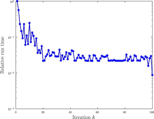As the number of iterations increases and the points $x_i^{\left(k\right)}$ converge, the initial guess $w_{\mathrm{i}\mathrm{n}\mathrm{i}\mathrm{t}}=w^{(k-1)}$ becomes better and better and consequently the optimisation step becomes quicker and quicker. This is illustrated in Figure 3, which shows the relative run time of each iteration for an example in which the relative sizes and relative proportions of small and large grains are the same as in Example 3.2 but the number of grains is $n=500$. We see that the total runtime of the algorithm is not proportional to the number of iterations $K$; most of the expense is in the first few iterations.

Figure 3. The relative run times for each optimisation step of Algorithm 2. In this example, the parameters are the same as those in Example 3.2, except that the number of grains is $n=500$. The relative proportion of small and large grains is the same as in Example 3.2 and the ratio of the size of the largest grain to the size of the smallest grain is 10. The initial seed locations are randomly distributed in the unit square. The y-axis displays $t_k/t_1$, where $t_k$ is the run time for the optimisation step of iteration $k$. After 12 iterations the time per iteration falls to below one-tenth the time of the first iteration, and after 18 iterations it falls to below one-twentieth. This is because the initial guess for the weights in the inner iteration is taken from the output of the previous outer iteration, and the quality of this guess improves as the number of iterations increases.

Note that for the first iteration, $k=1$, the initial guess $w_{\mathrm{i}\mathrm{n}\mathrm{i}\mathrm{t}}=0$ does not incorporate any information about the locations $x_i^{\left(0\right)}$. It is possible to improve the speed of the first iteration by using a more sophisticated choice of $w_{\mathrm{i}\mathrm{n}\mathrm{i}\mathrm{t}}$, e.g. using the multilevel methods of Mérigot [30] and Lévy [32], which generate a good initial guess $w_{\mathrm{i}\mathrm{n}\mathrm{i}\mathrm{t}}$ by solving a sequence of smaller optimisation problems with fewer grains. (For example, you can obtain a good initial guess $w_{\mathrm{i}\mathrm{n}\mathrm{i}\mathrm{t}}$ for $n$ grains by first solving a coarser problem with $n/2$ grains; you can obtain a good initial guess for $n/2$ grains by first solving a coarser problem with $n/4$ grains, etc.) We found that Mérigot's multilevel method [30] in 2D could halve the run time of iteration $k=1$ when there are $n=10,000$ grains. It is reported that Lévy's multilevel program GEOGRAM can handle one million grains in 3D [32, Table 4].

It is also possible to obtain a better initial guess $w_{\mathrm{i}\mathrm{n}\mathrm{i}\mathrm{t}}$ for iterations $k\ge 2$ as follows. The Lloyd step (6(6) $x_i^{\left(k\right)}:=\frac{1}{|L_i^{(k-1)}|}{\int }_{L_i^{(k-1)}}x\mathrm{d}x,$(6) ) of Algorithm 2 could be replaced with a damped Lloyd step of the form(17) $x_i^{\left(k\right)}:=(1-\lambda )x_i^{(k-1)}+\lambda \frac{1}{|L_i^{(k-1)}|}{\int }_{L_i^{(k-1)}}x\mathrm{d}x,$(17) where λ is a damping parameter between 0 and 1. The choice $\lambda =1$ corresponds to the Lloyd step (6(6) $x_i^{\left(k\right)}:=\frac{1}{|L_i^{(k-1)}|}{\int }_{L_i^{(k-1)}}x\mathrm{d}x,$(6) ). The closer $\lambda$ is to 0, the closer $x_i^{\left(k\right)}$ is to $x_i^{(k-1)}$, and so the better the associated initial guess $w_{\mathrm{i}\mathrm{n}\mathrm{i}\mathrm{t}}=w^{(k-1)}$. Therefore, the optimisation step is faster for smaller $\lambda$. On the other hand, the regularisation step has less effect for smaller $\lambda$, and it is necessary to increase the number of iterations $K$ to achieve the same amount of regularisation. For our purposes, the full Lloyd step $\lambda =1$ was sufficiently fast and so we did not try to optimise the choice of $\lambda$.

4.2.2. Choice of the tolerance

For simplicity, we chose the tolerance $\epsilon$ of the optimisation step of Algorithm 2 to be fixed at each iteration $k$ (recall that the optimisation step terminates when $\left|\mathrm{\nabla }{g}_k\right(w^{\left(k\right)}\left)\right|<\epsilon \underset{j}{min}{m}_j$). The algorithm could be sped up, however, by taking $\epsilon ={\epsilon }_k$ to depend on $k$. In order for Algorithm 2 to produce a Laguerre diagram with grains of given volumes up to a relative error of $\epsilon$, we only need the tolerance to be $\epsilon$ at the final iteration, ${\epsilon }_K=\epsilon$. For previous iterations, we could use a cruder tolerance: $\epsilon ={\epsilon }_K<{\epsilon }_{K-1}<\cdots <{\epsilon }_2<{\epsilon }_1$. It is tempting to think that the larger the tolerance, the faster the optimisation step. On the other hand, if ${\epsilon }_{k-1}$ is larger than ${\epsilon }_k$, then the initial guess $w_{\mathrm{i}\mathrm{n}\mathrm{i}\mathrm{t}}=w^{(k-1)}$ at iteration $k$ may be worse, and the optimisation step at iteration $k$ may be slower. So the tolerances ${\epsilon }_k$ must be chosen carefully. The choice of fixed tolerance ${\epsilon }_k=\epsilon$ for all $k$ is a simple, reliable option, which is why we used it.

4.2.3. Choice of the optimisation algorithm

The speed of the optimisation step depends of course not only on the choice of the initial guess $w_{\mathrm{i}\mathrm{n}\mathrm{i}\mathrm{t}}$ and the tolerance $\epsilon$, but also on the choice of the optimisation algorithm. For example, instead of using a quasi-Newton method as we did, one could use Newton's method. Newton's method tends to converge faster than quasi-Newton methods (quadratically rather than superlinearly), although it is harder to implement since it requires the second derivative of $g$ (whereas quasi-Newton methods only require the first derivative) [31].

It can be shown (see, e.g. [35]) that(18) $\frac{{\mathrm{\partial }}^{2}g}{\mathrm{\partial }{w}_i\mathrm{\partial }{w}_j}=-\frac{\mathrm{\partial }|L_i|}{\mathrm{\partial }{w}_j}=\left\{\begin{array}{cc}-\sum _{k\in N_i}\frac{a_{ik}}{2|x_i-x_k|}& \mathrm{i}\mathrm{f}i=j,\\ \frac{a_{ij}}{2|x_i-x_j|}& \mathrm{i}\mathrm{f}j\in N_i,\\ 0& \mathrm{o}\mathrm{t}\mathrm{h}\mathrm{e}\mathrm{r}\mathrm{w}\mathrm{i}\mathrm{s}\mathrm{e},\end{array}\right.$(18) where $a_{ij}$ is the area of the face between cell $i$ and cell $j$ and $N_i$ is the index set of the neighbours of cell $i$ (that is $j\in N_i$ if and only if cell $j$ and cell $i$ share a face). The pseudo-inverse of this Hessian matrix is used in a damped Newton method in [33, Algorithm 1], where fractions of a full Newton step are used in order to control the error reduction and the minimum volume of a cell (to stop cells disappearing). The authors prove that their damped Newton method converges globally with order 1 and locally with order 2 [33, Theorem 1.5].

4.3. Initialisation: effect on the spatial distribution

In this section, we discuss the initialisation step of Algorithms 1 and 2.

4.3.1. Initialisation of the seeds

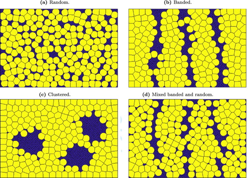
The locations of the generators $x_1,\dots ,x_n$ at the termination of Algorithm 2 are a strong function of the initial choice $x_1^{\left(0\right)},\dots ,x_n^{\left(0\right)}$. This simple observation gives us a great deal of control over the spatial distribution of the different sized grains. Examples of Algorithm 2 with different initial distributions of the generators $x_1^{\left(0\right)},\dots ,x_n^{\left(0\right)}$ are shown in Figure 4. In these examples, $\mathrm{\Omega }=[0,3]\times [0,2]$ and there are $n=1000$ grains. There are $n_1=800$ grains of size $x$ and $n_2=200$ grains of size $20x$. The tolerance is $\epsilon =0.01$ and the number of iterations of Algorithm 2 is $K=20$. The figure shows the output of Algorithm 2. The final spatial distribution of grains has some features in common with the spatial distribution of the initial generator locations.

Figure 4. Examples of more advanced microstructures: Coupling of size and spatial distributions with Algorithm 2. This figure shows the output of Algorithm 2 after $K=20$ iterations with different initial distributions for the seed locations. In all cases there are $n=1000$ grains with $n_1=800$ grains of size $x$ and $n_2=200$ grains of size $20x$ . (a) Random distribution of initial locations. Here the initial generator locations of the large and small grains are uniformly distributed over $\mathrm{\Omega }$. (b) Banded distribution of initial locations. Here, the different sized grains have initial generator locations that lie inside bands within $\mathrm{\Omega }$. The sizes of the bands have been chosen so that there are approximately equal numbers of small grains within each small-grain band and approximately equal numbers of large grains within each large-grain band. (c) Clustered distribution of initial locations. Here, the smaller grains have initial generator locations that lie inside non-overlapping discs. (d) A mixed distribution: the initial generators are such that the larger grains are arranged in bands and the smaller grains are a combination of the banded and random distributions.

A further example of controlling the spatial distribution of grains can be seen in Figure 5. In this example, $n=1000$ grains have areas drawn from a random distribution such that the ratio of the largest to the smallest grain size is at most 100. The Laguerre diagram in Figure 5(a) has the property that the grain sizes tend to increase from left to right. A variety of spatial distributions of grain sizes can be simulated by first distributing the seed locations appropriately. Figure 5(b) shows how a more complicated distribution can be produced.

Figure 5. Experiments to demonstrate a gradient in the distribution of grain sizes. Here, $n=1000$ grains have areas drawn from a uniform distribution such that the ratio of the largest to the smallest grain size is at most 100. The domain is $\mathrm{\Omega }=[0,3]\times [0,2]$. The results are shown after $K=20$ iterations and the grains are coloured according to their area. (a) The initial seed locations $x_1^{\left(0\right)},\dots ,x_n^{\left(0\right)}$ are distributed such that the $x$-coordinate increases with grain size. (b) The initial seed locations are distributed such that the larger grains are found in the middle of $\mathrm{\Omega }$.

4.3.2. Initialisation of the weights

The choice of $w^{\left(0\right)}$ in the initialisation step of Algorithm 2 is also important. One should choose $w_1^{\left(0\right)},\dots ,w_n^{\left(0\right)}$ so that the Laguerre diagram generated by $(x_1^{\left(0\right)},w_1^{\left(0\right)}),\dots ,(x_n^{\left(0\right)},w_n^{\left(0\right)})$ has no empty Laguerre cells. If there are empty cells then the regularisation step is not defined (there is division by zero in equation (6(6) $x_i^{\left(k\right)}:=\frac{1}{|L_i^{(k-1)}|}{\int }_{L_i^{(k-1)}}x\mathrm{d}x,$(6) ) if $L_i^{\left(0\right)}$ is empty). A good choice is $w^{\left(0\right)}=0$ since then the Laguerre diagram generated by $(x_1^{\left(0\right)},w_1^{\left(0\right)}),\dots ,(x_n^{\left(0\right)},w_n^{\left(0\right)})$ is a Voronoi diagram and so has no empty cells, whatever the choice of $x_1^{\left(0\right)},\dots ,x_n^{\left(0\right)}$.

4.4. Stopping criteria

In Algorithm 2, the user must specify the number of regularisation steps $K$. As we discussed in Section 3.1, for large values of $K$ the Laguerre diagram resulting from Algorithm 2 is approximately a centroidal Laguerre diagram, which means that each seed $x_i^{\left(K\right)}$ is approximately the centre of mass of its Laguerre cell $L_i^{\left(K\right)}$. Centroidal Laguerre diagrams tend to have very regular-shaped cells, e.g. in 2D if the grains all have the same target areas, $m_i=1/n$, and if $n$ and $K$ are large, then the Laguerre diagram looks locally like a regular hexagonal tiling. Indeed for steel microstructures, we found that if $K$ is too large, then Algorithm 2 tends to produce grains that are too ‘round’ compared to EBSD measurements of grain aspect ratios.

Instead of fixing the number of steps $K$ in advance, the user could terminate the algorithm whenever some measure of the maximum grain aspect ratio falls below a critical threshold. For example, the aspect ratio of grain can be measured using the ratio of its largest and smallest principal moments of inertia, or using the ratio of the radii of circumscribed and inscribed balls, or using its sphericity [46], which is the ratio of the surface area of the volume-equivalent sphere to the surface area of the grain.

The user may also want to terminate the algorithm if the distance $|x_i^{\left(k\right)}-x_i^{(k-1)}|$ moved by the seeds from one iteration to the next falls below some threshold. The Laguerre diagram $\left\{L_i^{\left(k\right)}\right\}$ tends to evolve slowly with $k$ when $k$ is large, as illustrated in Figure 2, and the evolution can slow down dramatically when there is a T1 topological transition (to borrow a term from foam dynamics). This topological transition involves a change of cell neighbour relations; in 2D this is via coalescence of two triple junctions of cell boundaries. So, in general, there is little to be gained from performing a large number of regularisation steps, especially since our aim is not to produce a centroidal Laguerre diagram, but rather to produce a physically realistic microstructure. (If on the other hand, the user's aim is to produce centroidal Laguerre diagrams, then it would be better to use the quasi-Newton method of [36], which converges superlinearly as opposed to the linear convergence of Lloyd's algorithm.)

5. Examples

This section includes some large examples in 3D to illustrate the capabilities of our algorithms.

Example 5.1

(Run time tests):

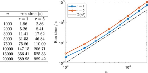
Figure 6 gives some run times of Algorithm 2 for creating monodisperse and polydisperse periodic Laguerre diagrams in 3D. Here Algorithm 2 has been used to create $n/2$ grains of volume $x$ and $n/2$ grains of volume $rx$, for $r=1$ and $r=5$, in a cube of side length 100 with error tolerance $\epsilon =0.01$. We see that the run time grows roughly quadratically in the range $n=2000$ to $n=5000$, for both the monodisperse (single phase) case $r=1$ and the polydisperse (dual phase) case $r=5$. This could be expected since the cost of each iteration of the BFGS method used by fminunc is $\mathcal{O}\left(n^2\right)$ (a matrix-vector multiplication). Also the worst-case optimal time it takes to compute a Laguerre diagram of $n$ cells is $\mathcal{O}\left(n^2\right)$ in 3D, although we found that in these examples the cost of computing the Laguerre diagrams was sub-quadratic (but super-linear); see also the discussion in Section 4.1. For $n>5000,$ the run time grows a little faster than $\mathcal{O}\left(n^2\right)$. Observe also from Figure 6 that it is about 50% more expensive to compute dual phase RVEs ($r=5$) than single phase RVEs ($r=1$).

Figure 6. Run times in seconds of Algorithm 2 for creating monodisperse (single phase) and polydisperse (dual phase) periodic RVEs in 3D. There are $n/2$ grains of volume $x$ and $n/2$ grains of volume $rx$ in a cube of side length 100 with at most $1\text{\%}$ error ($\epsilon =0.01$) in the volumes of the grains ($r=1$ corresponds to a single phase material, $r=5$ corresponds to a dual phase material, $x$ is chosen such that the total volume of the grains equals the volume of the box). We used $K=5$ regularisation steps, and the initial seed locations $x_1^{\left(0\right)},\dots ,x_n^{\left(0\right)}$ were chosen randomly from a uniform distribution. The simulations were performed on an Intel Xeon E5-1620V3 (3.5 GHz, 4 cores, 8 threads). The graph on the right has a log–log scale. The black dotted line is the graph of the function $c{n}^2$, where $c$ is a constant. It is included to illustrate how the run times grow with $n$.

Example 5.2

(Generating a periodic RVE of an IF steel):

Figure 7 shows an example of a periodic Laguerre diagram created using Algorithm 2. The target volumes $m_i$ are taken from a 3D EBSD measurement of an IF (interstitial free) steel (EN 10130 grade DC06). There are $n=9211$ grains in a box of dimensions $670\mu \mathrm{m}\times 80\mu \mathrm{m}\times 480\mu \mathrm{m}$. We took the initial seed locations $x_1^{\left(0\right)},\dots ,x_n^{\left(0\right)}$ to be the centres of mass of the grains from the EBSD data, and performed $K=10$ regularisation steps with a tolerance of $0.5\text{\%}$ ($\epsilon =0.005$). 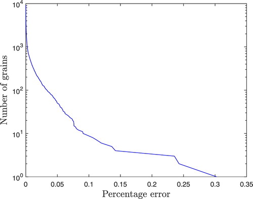The grains in Figure 7 are coloured according to their lattice orientations by mapping the three Euler angles linearly to RGB values. The orientations were taken from the EBSD data. Figure 8 shows that the volumes of all the grains are correct to within $0.5\text{\%}$, and most volumes are correct to within $0.05\text{\%}$.

Figure 7. A periodic RVE of an IF steel with $n=9211$ grains, generated using Algorithm 2 (see Example 5.2). The grains are coloured according to their lattice orientations.

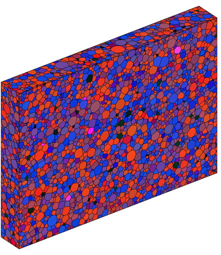
Figure 8. The complementary cumulative number distribution of the percentage error of the volumes of the grains for Example 5.2. For a percentage error $x$, we plot the number of grains that have a volume percentage error at least $x$. Most of the grain volumes have percentage error less than $0.05\text{\%}$, which is an order of magnitude below the tolerance of $0.5\text{\%}$ ($\epsilon =0.005$). In this example, the maximum percentage error is $0.30\text{\%}$.

Example 5.3

(Fitting a Laguerre diagram to EBSD measurements):

The main aim of this paper is to create Laguerre diagrams with given volume distributions for use in computational homogenisation simulations. We briefly mention, however, how Algorithm 1 can be used to fit a Laguerre diagram to EBSD data of grain volumes and centroids. Figure 9 is an example of a non-periodic Laguerre diagram fitted to a 3D EBSD measurement of an IF steel (EN 10130 grade DC06) with $n=9211$ grains in a box of dimensions $670\mu \mathrm{m}\times 80\mu \mathrm{m}\times 480\mu \mathrm{m}$ (this is the same EBSD data used in the previous example). In the initialisation step of Algorithm 1, we took $x_1,\dots ,x_n$ to be the centroids of the grains from the EBSD data. The target volumes $m_i$ were also taken from the EBSD data. We used a tolerance of $1\text{\%}$ ($\epsilon =0.01$). As in the previous example, the grains in Figure 9 are coloured according to their lattice orientation. Observe that Figure 9 is less regular than Figure 7, which is because Algorithm 1 is missing the regularisation steps of Algorithm 2. Figure 10 shows that the volumes of all the grains are correct to within $0.56\text{\%}$, and most volumes are correct to within $0.1\text{\%}$.Figure 11 shows the complementary cumulative number distribution of the relative errors of the centroids. The relative error for grain $i$ is defined by(19) $\frac{|x_i-c_i|}{r_i},$(19) where $x_i$ is the centroid of grain $i$ from the EBSD data, $c_i$ is the centroid of the Laguerre cell $L_i$, and $r_i$ is the radius of a sphere of volume $m_i$, where $m_i$ is the target volume of grain $i$. This definition of relative error was proposed by [9]. As expected, the centroid errors are higher than the volume errors since Algorithm 1 does not directly try to fit the centroids. To be precise, the optimisation step of Algorithm 1 only minimises the fitting error of the volumes; the centroid fitting error is not minimised (the centroids do not appear in the objective function $g$). However, the centroid measurements are used in the initialisation step of Algorithm 1. The relative error of 79% of the grain centroids is less than 1 and the relative error of 93% of the grain centroids is less than 2.The run time for this example was 376 s on an Intel Xeon E5-1620V3 (3.5 GHz, 4 cores, 8 threads) with the initial guess $(w_{\mathrm{i}\mathrm{n}\mathrm{i}\mathrm{t}}{)}_i=(3m_i/\left(4\pi \right){)}^{2/3}$, which was inspired by sphere-packing methods [4,8,10,18].

Figure 9. A non-periodic Laguerre diagram fitted to 3D EBSD data of an IF steel using Algorithm 1 (see Example 5.3). The grains are coloured according to their lattice orientations. The volume distribution has a fitting error of less than $1\text{\%}$. The texture intensity inherits the same fitting error.

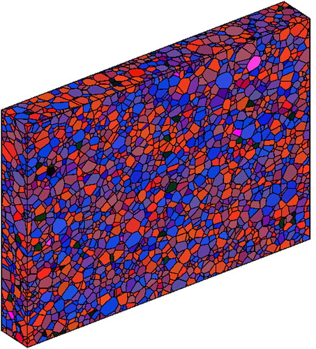
Figure 10. The complementary cumulative number distribution of the percentage error of the volumes of the grains for Example 5.3. For a percentage error $x$, we plot the number of grains with volume percentage error at least $x$. The largest percentage error is $0.56\text{\%}$ and the second largest is $0.43\text{\%}$. All the other percentage errors are below $0.34\text{\%}$.

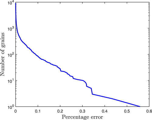
Figure 11. The complementary cumulative number distribution of the relative error of the centroids of the grains for Example 5.3. For a relative error $x$, we plot the number of grains with centroid relative error at least $x$. The maximum relative error is 11.16%, which is worse than the result given in [9, Figure 9], although for most of the grains the relative errors are comparable: 7278 of the 9211 grains have a relative error less than 1, and 8596 of the 9211 grains have a relative error less than 2.

Example 5.4

(Generating a dual phase RVE with a banded microstructure):

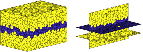
Figure 12 shows an example of a periodic, dual phase Laguerre diagram with a band of small grains in the centre, generated using Algorithm 2. There are $n=10,000$ grains: 8000 grains of volume $x$ and 2000 grains of volume $20x$ (where $x$ was chosen so that the total volume of the grains equals the volume of the box). We used $K=20$ regularisation steps and a volume tolerance of $1\text{\%}$. The grains are coloured according to their volume. In order to obtain the banded structure, we placed the initial seeds $x_1^{\left(0\right)},\dots ,x_n^{\left(0\right)}$ at random within bands of the correct volume. We see from Figure 12 that these bands were largely preserved by the regularisation steps.

Figure 12. A periodic RVE of a dual phase material with a banded microstructure (see Example 5.4).

Example 5.5

(Generating an RVE with a log-normal distribution of grain volumes):

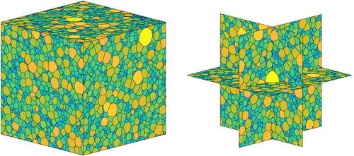
Figure 13 shows an example of a periodic Laguerre diagram generated by Algorithm 2, in which the grains have volumes that are log-normally distributed. There are $n=10,000$ grains. We used $K=5$ regularisation steps and a volume tolerance of $1\text{\%}$. The grains are coloured by their volume, using a log scale. We placed the initial seeds $x_1^{\left(0\right)},\dots ,x_n^{\left(0\right)}$ at random. The target volumes were generated by drawing 10,000 samples $r_i$ from a log-normal distribution with mean 1 and standard derivation 0.35 (these correspond to the log-normal parameters $\sigma =(\log (1+{0.35}^2){)}^{1/2}=0.34$ and $\mu =-{\sigma }^2/2$). The target volumes were defined by(20) $m_i=\frac{r_i^3}{L_1{L}_2{L}_3{\displaystyle \sum _{j=1}^n{r}_j^3}},$(20) where the $L_i$ are the side-lengths of the domain $\mathrm{\Omega }=[0,L_1]\times [0,L_2]\times [0,L_3]$. For large $n$ these target volumes are approximately log-normally distributed with coefficient of variation (the ratio of standard variation to mean) of(21) $\frac{1}{3}\sqrt{\exp \left(9{\sigma }^2\right)-1}.$(21) The algorithm took 669 s using the same machine as above. Observe from Example 5.1 that Algorithm 2 took only 147 s to produce a monodisperse RVE and 207 s to produce a dual phase RVE with the same number of grains ($n=10,000$) and the same number of regularisation steps ($K=5$). Therefore, the run time of Algorithm 2 increases as the RVE becomes more polydisperse.

Figure 13. An RVE in which the grain volumes have approximately log-normal distribution (see Example 5.5). There are $n=10,000$ grains in the cubic cell. The coefficient of variation of the volumes (the ratio of the standard deviation to the mean) is 1.4. Cross-sections of the cell are also shown, showing the distribution of sizes throughout the cell.

6. Discussion

The advantages of our method are

• it is fast;

• it can create Laguerre diagrams with grains of exact volumes, in principle of any desired tolerance up to machine precision;

• it gives some control over the spatial distribution of the grains;

• it can create periodic and non-periodic Laguerre diagrams.

The disadvantages of our method are

• it provides no direct control over the centroids of the grains or their morphology, e.g. their aspect ratio;

• it is currently limited to Laguerre diagrams and so the grains cannot have curved boundaries or be non-convex.

We now discuss these advantages and disadvantages in more detail, give evidence in support of our claims, and compare our method with others in the literature.

6.1. Controlling grain volumes: speed and accuracy

Figure 6 shows that we can create Laguerre diagrams in 3D with up to 20,000 grains in around 10 min on a standard desktop PC (without using parallel computation), where the volumes of the grains are correct to within $1\text{\%}$. For 10,000 grains, we require as little as 2.5 min (see Figure 6), although the time depends on the regularity of the microstructure and whether the material is monodisperse or polydisperse; in Example 5.3 it took 6.25 min for 9211 grains and in Example 5.5 it took about 11 min for 10,000 grains.

In our implementation of Algorithm 2, we simply used MATLAB's all-purpose fminunc optimisation algorithm. With modern, customised optimal transport optimisation algorithms such as [32,33] it should be possible to use our method to generate Laguerre diagrams with given volume distributions with 100,000 grains in a few minutes [32, Table 3] or even one million grains in less than an hour [32, Table 4].

We now compare this with the speed of other algorithms. It is difficult to make a direct comparison in some cases since different methods fit different geometric properties.

In [9], a stochastic optimisation method (the cross-entropy method) is used to solve a non-convex optimisation problem to fit a Laguerre diagram to 3D XRD measurements of grain volumes and centroids. The authors report simulation times (performed using parallel computation) of 19.2 h for 1439 grains and 122.3 h for 8063 grains. Note that it is hard to compare their run times with ours since they also fitting centroids; their method does not try to fit the volumes exactly like we do, but rather obtain a good fit for both volumes and centroids, and their method can produce empty Laguerre cells (grains with volume zero). While the main focus of our paper is to fit volumes only, we gave an example of fitting volumes and centroids in Example 5.3, where we fit a Laguerre diagram to 3D EBSD measurements of an IF steel with 9211 grains. The run time is 6.25 min and the volumes are correct to within $0.56\text{\%}$. The centroid errors of most of the grains are comparable to those given in [9, Figure 9], although overall our method does worse than [9] at centroid fitting, as expected.

Sphere-packing methods are popular for fitting Laguerre diagrams to volume distributions [4,8,10,18]. For $n$ non-overlapping spheres $S_1,\dots ,S_n$ with centres $x_1,\dots ,x_n$ and radii $r_1,\dots ,r_n$, the Laguerre diagram with seeds $x_i$ and weights $w_i=r_i^2$ has the property that cell $L_i$ contains sphere $S_i$. Therefore, the volume of $L_i$ is at least the volume of $S_i$. The idea of sphere-packing methods is that if the spheres are close-packed, then the volumes of the Laguerre cells are approximately equal to the volumes of the solid spheres. The disadvantage of this method is that it is inexact and computationally expensive since the sphere-packing problem is NP hard [47]. Nevertheless, this method provided us with inspiration for a good initial guess for the optimisation simulation in Example 5.3 (see also Section 4.2.1).

In [1], a method is proposed for fitting grain measurements with generalised balanced power diagrams (GBPDs), which are a generalisation of Laguerre diagrams. GBPDs are generated by triples $(x_i,w_i,A_i)$ of seeds $x_i$, weights $w_i$, and positive definite matrices $A_i$; the matrices $A_i$ give some control over the aspect ratio of the generalised Laguerre cells; the case $A_i=I$ for all $i$ corresponds to a standard Laguerre diagram. The advantage of GBPDs is that they give a high degree of control over the morphology of the grains [1, Figures 1–6]. The disadvantage is that they are hard to compute. In [1], the authors approximate GBPDs by voxels, and they fit discretised GBPDs to grain measurements by solving a high-dimensional linear programming problem, where the number of unknowns equals the number of grains multiplied by the number of voxels. It is reported that to fit a discretised GBPD to 109 grains in 3D took around 6 h on a standard laptop (this involved solving a linear programming problem with over 77 million variables and 78 million constraints) [1, Section 5.3]. Again, it is not possible to make a direct comparison of these run times with the ones presented here since grain volumes and morphology are fitted in [1], not only grain volumes like here.

A heuristic method for approximately fitting GBPDs to measurements of grain volumes, centroids and aspect ratios was proposed in [13]. Their method entirely avoids solving an optimisation problem; it includes explicit formulas for the generators $(x_i,w_i,A_i)$ in terms of the data. It is reported in [13] that the method is comparable in accuracy with the optimisation methods of [1,11,21] but takes a small fraction of the computation time. No run times or volume errors are reported in [13] precluding a more precise comparison with our method. Like the sphere-packing method, this heuristic method could be used for generating good initial guesses for optimisation methods.

6.2. Controlling grain geometry

The main goal of our method is to fit grain volumes quickly and accurately. Unlike other methods [1,9,11–13,21,24], it is not specifically designed for fitting grain morphology. We now discuss to what extent we can control the geometry of Laguerre diagrams.

Our method gives some control over the spatial distribution of the grains, as shown in Figures 4, 5 and 12, where we create microstructures with bands, clusters, and size gradients.

Several authors use grain centroids as a measure of fitting-error when fitting Laguerre diagrams to data measurements, e.g. [9,13]. We show how we can approximately fit grain centroids to 3D EBSD data in Example 5.3, although the accuracy is much lower than the volume accuracy.

In its current form, our method gives no direct control over the aspect ratio of the grains. Like the sphere-packing method, Algorithm 2 tends to produce grains that are too round compared to grains typically seen in metals; see Section 4.4.

Nevertheless, there are several ways how our method could be generalised to give more control over the morphology of the grains. For example, by combining our method with multilevel Voronoi diagrams [5,17] we could maintain control over the volume of the grains while producing more realistic RVEs with non-convex and elongated grains. The idea would be to first use Algorithm 2 to create a Laguerre diagram with $N$ ‘micro-grains’ of equal volume for large $N$. Then we would glue together the micro-grains into non-convex ‘macro-grains’. By choosing which micro-grains to glue, we would control the volume and the morphology of the macro-grains. (The multilevel Voronoi method glues together two micro-grains if their generators lie in the same Voronoi cell of a ‘coarser’ Voronoi diagram with fewer generators.)

In principle, our algorithms can also be generalised very easily to produce GBPDs with grains of given volumes (up to any desired tolerance) by modifying the objective functions $g$ and $g_k$ in Algorithms 1 and 2 (simply replace the Laguerre cells $L_i$ with generalised Laguerre cells, and replace the isotropic distances $|x-x_i|$ with anisotropic distances $|x-x_i{|}_{A_i}$). This would again allow us to control both the volumes and the aspect ratio of the grains. In practice, however, it is expensive to compute GBPDs to high accuracy; discretising them with voxels greatly increases the cost of the algorithm. Without developing new computational geometry algorithms for the efficient computation of GBPDs, this limits the method to a small number of grains or greatly increases the run time (cf. the run time of 6 h for 109 grains in 3D in [1]).

Since our method is currently limited to Laguerre diagrams, the grains cannot have curved boundaries or be non-convex. Curved grain boundaries can be created using additively weighted Voronoi diagrams (Apollonius diagrams) [27], anisotropic diagrams [2], or GBPDs [1,12,13,21], although these are all more costly to compute than Laguerre diagrams. Algorithms 1 and 2 can also be modified to produce Apollonius diagrams with grains of given volumes (in the definition of the objective functions $g$ and $g_k$ simply replace the Laguerre cells $L_i$ with Apollonius cells, and replace the squared distances $|x-x_i{|}^2$ with non-squared distances $|x-x_i|$) but again the implementation cost is an obstacle at the present time. We plan to explore this and the above generalisations in a future paper.

7. Conclusions

In this paper, we introduced a fast optimisation method for generating Laguerre diagrams with user-defined grain size distributions. The volumes of the grains can be controlled exactly (to within any given tolerance). We produced industrially relevant examples of RVEs with up to 20,000 grains with only $1\text{\%}$ volume error in the order of minutes on a standard desktop PC. We also demonstrated how the spatial and texture distribution of the grains can be partially controlled. Our algorithms can create both non-periodic Laguerre diagrams (for data fitting) and periodic Laguerre diagrams (for generating RVEs of polycrystalline metals or solid foams for computational homogenisation).

Acknowledgments

The authors would like to thank Carola Celada-Casero for useful discussions.

Disclosure statement

No potential conflict of interest was reported by the author(s).

Additional information

Funding

D.P.B. would like to thank the Engineering and Physical Sciences Research Council (EPSRC) for financial support via the grant EP/R013527/1, EP/R013527/2 Designer Microstructure via Optimal Transport Theory. Some of the work of D.P.B. was carried out at Durham University. The work on generating 3D EBSD data has received funding from the European Union's Horizon 2020 research and innovation programme Euratom research and training programme 2014–2018 under grant agreement No 709418 MuSTMeF.

Notes

1 Technical remark: It can be shown that evaluating the optimal transport (Wasserstein) distance $W_2({\chi }_{\mathrm{\Omega }},\sum _i{m}_i{\delta }_{x_i})$ between the Lebesgue measure and a discrete measure generates a partition of $\mathrm{\Omega }$ into Laguerre cells of size $m_1,\dots ,m_n$.

Appendix. Proof that Algorithm 2 is energy-decreasing and convergent

Throughout this section, we assume that $\mathrm{\Omega }\subset {\mathbb{R}}^d$ is compact.

First, we prove that Algorithm 2 is energy-decreasing, Equation (16(16) $E(x_1^{(k+1)},\dots ,x_n^{(k+1)})\le E(x_1^{\left(k\right)},\dots ,x_n^{\left(k\right)}).$(16) ). Recall that if $U$ is a compact subset of ${\mathbb{R}}^d$ with centroid $c\left(U\right)$, then(A1) $\underset{z\in {\mathbb{R}}^d}{min}{\int }_U|x-z{|}^2\mathrm{d}x={\int }_U|x-c\left(U\right){|}^2\mathrm{d}x.$(A1) This follows from the fact that the function $z\mapsto {\int }_U|x-z{|}^2\mathrm{d}x$ is strictly convex with unique critical point $c\left(U\right)$. By Equation (13(13) $E(x_1,\dots ,x_n)=\sum _{i=1}^n{\int }_{L_i}|x-x_i{|}^2\mathrm{d}x,$(13) ) and by the way $\left\{\right(x_i^{\left(k\right)},w_i^{\left(k\right)}){\}}_{i=1}^n$ is constructed using Algorithm 2,(A2) $E(x_1^{\left(k\right)},\dots ,x_n^{\left(k\right)})=\sum _{i=1}^n{\int }_{L_i^{\left(k\right)}}|x-x_i^{\left(k\right)}{|}^2\mathrm{d}x,$(A2) where $\{L_i^{\left(k\right)}{\}}_{i=1}^n$ is the Laguerre diagram with generators $\left\{\right(x_i^{\left(k\right)},w_i^{\left(k\right)}){\}}_{i=1}^n$. Therefore,(A3) $\begin{array}{rl}& E(x_1^{\left(k\right)},\dots ,x_n^{\left(k\right)})\stackrel{\left(A1\right)}{\ge }\sum _{i=1}^n{\int }_{L_i^{\left(k\right)}}|x-c\left(L_i^{\left(k\right)}\right){|}^2\mathrm{d}x\\ & =\sum _{i=1}^n{\int }_{L_i^{\left(k\right)}}|x-x_i^{(k+1)}{|}^2\mathrm{d}x(\mathrm{r}\mathrm{e}\mathrm{g}\mathrm{u}\mathrm{l}\mathrm{a}\mathrm{r}\mathrm{i}\mathrm{s}\mathrm{a}\mathrm{t}\mathrm{i}\mathrm{o}\mathrm{n}\mathrm{s}\mathrm{t}\mathrm{e}\mathrm{p}\mathrm{o}\mathrm{f}\mathrm{A}\mathrm{l}\mathrm{g}.2)\\ & \stackrel{\left(12\right)}{\ge }E(x_1^{(k+1)},\dots ,x_n^{(k+1)}).\end{array}$(A3) This proves (16(16) $E(x_1^{(k+1)},\dots ,x_n^{(k+1)})\le E(x_1^{\left(k\right)},\dots ,x_n^{\left(k\right)}).$(16) ). The inequalities above are strict unless $x_i^{\left(k\right)}=x_i^{(k+1)}$ for all $i$, which means that $(x_1^{\left(k\right)},\dots ,x_n^{\left(k\right)})$ is a fixed point of Algorithm 2.

Next, we prove a weak global convergence result of the form [48, Theorem 3.8], where convergence of the classical Lloyd algorithm was proved. Weak global convergence means that $\mathrm{\nabla }E(x_1^{\left(k\right)},\dots ,x_n^{\left(k\right)})\to 0$ as $k\to \mathrm{\infty }$ and that any convergent subsequence of $(x_1^{\left(k\right)},\dots ,x_n^{\left(k\right)})$ converges to a critical point of $E$, namely to a centroidal Laguerre diagram. This convergence is called weak because it does not guarantee convergence of the whole sequence $(x_1^{\left(k\right)},\dots ,x_n^{\left(k\right)})$ (different subsequences could converge to different critical points).

By construction $x_i^{\left(k\right)}$ is the centroid of the convex set $L_i^{(k-1)}$, which has volume $m_i$. Therefore, by [48, Lemma 3.2], the distance between $x_i^{\left(k\right)}$ and $\mathrm{\partial }{L}_i^{(k-1)}$ has a lower bound of $C{m}_i^2/\mathrm{d}\mathrm{i}\mathrm{a}\mathrm{m}(\mathrm{\Omega }{)}^{2d-1}$ where $C=1/1024$. Therefore, the closest that two generators $x_i^{\left(k\right)}$ and $x_j^{\left(k\right)}$ can be is $2C{m}^2/\mathrm{d}\mathrm{i}\mathrm{a}\mathrm{m}(\mathrm{\Omega }{)}^{2d-1}$ where $m=\underset{i}{min}{m}_i$. Note that this bound is independent of the iteration number $k$. Therefore, the iterates $(x_1^{\left(k\right)},\dots ,x_n^{\left(k\right)})$ lie in the compact set(A4) $\left\{\right(x_1,\dots ,x_n)\in {\mathrm{\Omega }}^n:|x_i-x_j|\ge 2C{m}^2/\mathrm{d}\mathrm{i}\mathrm{a}\mathrm{m}(\mathrm{\Omega }{)}^{2d-1}\mathrm{\forall }i,j\}.$(A4) Owing to this compactness and the energy-decreasing property of Algorithm 2, we have weak global convergence of $(x_1^{\left(k\right)},\dots ,x_n^{\left(k\right)})$; see the Global Convergence Theorem in [49, p. 206] or [35, proof of Theorem 3.3].

Finally, we prove a strong convergence result, namely that the whole sequence $(x_1^{\left(k\right)},\dots ,x_n^{\left(k\right)})$ produced by Algorithm 2 converges to a critical point of $E$. We are only able to prove this, however, under the following generic assumption: There are only finitely many centroidal Laguerre diagrams with the same energy $E$. More precisely, we assume that, for all $M>0$,(A5) $\mathrm{\#}\left\{(x_1,\dots ,x_n)\in {\mathrm{\Omega }}^n:\mathrm{\nabla }E(x_1,\dots ,x_n)=0,E(x_1,\dots ,x_n)=M\right\}<\mathrm{\infty }.$(A5) This assumption is expected to hold for ‘generic’ domains $\mathrm{\Omega }$ and masses $m_1,\dots ,m_n$ [35, Remark 3.4], [50, p. 107], however, there are examples where it fails. For example, if $\mathrm{\Omega }$ is a disc, $n=2$ and $m_1=m_2$, then there are infinitely many critical points of $E$ with the same energy by the rotational symmetry of $\mathrm{\Omega }$. Note that if $E$ satisfies the generic condition of being a Morse function (having no degenerate critical points), then its critical points are isolated. Since they lie in the compact set (A4(A4) $\left\{\right(x_1,\dots ,x_n)\in {\mathrm{\Omega }}^n:|x_i-x_j|\ge 2C{m}^2/\mathrm{d}\mathrm{i}\mathrm{a}\mathrm{m}(\mathrm{\Omega }{)}^{2d-1}\mathrm{\forall }i,j\}.$(A4) ) there are only finitely many of them, and so assumption (A5(A5) $\mathrm{\#}\left\{(x_1,\dots ,x_n)\in {\mathrm{\Omega }}^n:\mathrm{\nabla }E(x_1,\dots ,x_n)=0,E(x_1,\dots ,x_n)=M\right\}<\mathrm{\infty }.$(A5) ) is satisfied.

The Monotone Convergence Theorem implies that the whole sequence $E(x_1^{\left(k\right)},\dots ,x_n^{\left(k\right)})$ converges (because Algorithm 2 is energy-decreasing and $E$ is bounded below by zero). In addition $E$ is continuous, and so every accumulation point of $(x_1^{\left(k\right)},\dots ,x_n^{\left(k\right)})$ has the same energy $E$. Moreover, by the global weak convergence result above, every accumulation point is a critical point of $E$. Therefore, assumption (A5(A5) $\mathrm{\#}\left\{(x_1,\dots ,x_n)\in {\mathrm{\Omega }}^n:\mathrm{\nabla }E(x_1,\dots ,x_n)=0,E(x_1,\dots ,x_n)=M\right\}<\mathrm{\infty }.$(A5) ) ensures there are only finitely many accumulation points.

We now complete the proof following the idea from [50, proof of Theorem 2.5]. Assume for contradiction that the sequence $X^{\left(k\right)}:=(x_1^{\left(k\right)},\dots ,x_n^{\left(k\right)})$ does not converge. Since it only has finitely many accumulation points, there exist distinct accumulation points $Y:=(y_1,\dots ,y_n)$, $Z:=(z_1,\dots ,z_n)$ and distinct subsequences $X^{\left(k_j\right)}:=(x_1^{\left(k_j\right)},\dots ,x_n^{\left(k_j\right)})$, $X^{\left(k_l\right)}:=(x_1^{\left(k_l\right)},\dots ,x_n^{\left(k_l\right)})$ such that $X^{\left(k_j\right)}\to Y$, $X^{\left(k_l\right)}\to Z$, and $k_l=k_j+1$, i.e. the sequence $X^{\left(k\right)}$ ‘jumps’ between the two subsequences infinitely many times. (Note that such subsequences may not exist if there are infinitely many accumulation points.) Let $\delta =|Y-Z|>0$ and let $T:{\mathrm{\Omega }}^n\to {\mathrm{\Omega }}^n$ denote the continuous map that sends $(x_1,\dots ,x_n)$ to $\left(c\right(L_1),\dots ,c(L_n\left)\right)$, where $\left\{L_i\right\}$ is the Laguerre diagram with seeds $(x_1,\dots ,x_n)$ and cells of volume $m_1,\dots ,m_n$. In other words, $X^{(k+1)}=T\left(X^{\left(k\right)}\right)$. Moreover, $T\left(Y\right)=Y$ and $T\left(Z\right)=Z$. Then (A6) $\begin{array}{rl}& \delta =|Y-Z|\\ & \le |Y-X^{\left(k_j\right)}|+|X^{\left(k_j\right)}-X^{\left(k_l\right)}|+|X^{\left(k_l\right)}-Z|\\ & =|Y-X^{\left(k_j\right)}|+|X^{\left(k_j\right)}-T\left(X^{\left(k_j\right)}\right)|+|X^{\left(k_l\right)}-Z|.& \left(\mathrm{A}6\right)\end{array}$(A6) By taking $j,l\to \mathrm{\infty }$ in the right-hand side, and using the continuity of $T$, we find that $\delta =0$, which is a contradiction. Therefore, the whole sequence $(x_1^{\left(k\right)},\dots ,x_n^{\left(k\right)})$ converges to a critical point of $E$. Moreover, this critical point must a local minimum point or a saddle point of $E$ by the energy-decreasing property. This completes the proof.

References

- A. Alpers, A. Brieden, P. Gritzmann, A. Lyckegaard, and H.F. Poulsen, Generalized balanced power diagrams for 3D representations of polycrystals, Philos. Mag. 95 (2015), pp. 1016–1028. Available at https://doi.org/10.1080/14786435.2015.1015469.
- H. Altendorf, F. Latourte, D. Jeulin, M. Faessel, and L. Saintoyant, 3D reconstruction of a multiscale microstructure by anisotropic tessellation models, Image Anal. Stereol. 33 (2014), pp. 121–130. Available at https://www.ias-iss.org/ojs/IAS/article/view/1090. doi: 10.5566/ias.v33.p121-130
- J. Barker, G. Bollerhey, and J. Hamaekers, A multilevel approach to the evolutionary generation of polycrystalline structures, Comput. Mater. Sci. 114 (2016), pp. 54–63. Available at http://www.sciencedirect.com/science/article/pii/S0927025615007259. doi: 10.1016/j.commatsci.2015.11.018
- D. Depriester and R. Kubler, Radical Voronoi tessellation from random pack of polydisperse spheres: prediction of the cells' size distribution, Computer-Aided Des. 107 (2019), pp. 37–49. Available at https://doi.org/10.1016/j.cad.2018.09.001.
- P.J.J. Kok and F.N.M. Korver. Modelling of complex microstructures in multi-phase steels: geometric considerations for building an RVE, Proceedings of the 10th International Conference on Computational Plasticity, Barcelona, 2009.
- A. Liebscher, Laguerre approximation of random foams, Philos. Mag. 95 (2015), pp. 2777–2792. Available at https://doi.org/10.1080/14786435.2015.1078511.
- A. Leonardi, P. Scardi, and M. Leoni, Realistic nano-polycrystalline microstructures: beyond the classical Voronoi tessellation, Philos. Mag. 92 (2012), pp. 986–1005. Available at https://doi.org/10.1080/14786435.2011.637984.
- A. Lyckegaard, E.M. Lauridsen, W. Ludwig, R.W. Fonda, and H.F. Poulsen, On the use of Laguerre tessellations for representations of 3d grain structures, Adv. Eng. Mater. 13 (2011), pp. 165–170. Available at https://onlinelibrary.wiley.com/doi/abs/10.1002/adem.201000258.
- L. Petrich, J. Staněk, M. Wang, D. Westhoff, L. Heller, P. Šittner, C.E. Krill III, V. Beneš, and V. Schmidt, Reconstruction of grains in polycrystalline materials from incomplete data using Laguerre tessellations, Microsc. Microanal. 25 (2019), pp. 743–752. Available at https://doi.org/10.1017/S1431927619000485.
- I. Pérez, M. Muniz de Farias, M. Castro, R. Roselló, C. Recarey Morfa, L. Medina, and E. Oñate, Modeling polycrystalline materials with elongated grains, Int. J. Numer. Methods. Eng. 118 (2019), pp. 121–131. Available at https://onlinelibrary.wiley.com/doi/abs/10.1002/nme.6004.
- A. Spettl, T. Brereton, Q. Duan, T. Werz, C.E. Krill III, D.P. Kroese, and V. Schmidt, Fitting Laguerre tessellation approximations to tomographic image data, Philos. Mag. 96 (2016), pp. 166–189. Available at https://doi.org/10.1080/14786435.2015.1125540.
- O. Šedivý, D. Westhoff, J. Kopeček, C.E. Krill III, and V. Schmidt, Data-driven selection of tessellation models describing polycrystalline microstructures, J. Stat. Phys. 172 (2018), pp. 1223–1246. Available at https://doi.org/10.1007/s10955-018-2096-8.
- K. Teferra and D.J. Rowenhorst, Direct parameter estimation for generalised balanced power diagrams, Philos. Mag. Lett. 98 (2018), pp. 79–87. Available at https://doi.org/10.1080/09500839.2018.1472399.
- Y. Wu, J. Cao, and Z. Fan, Chord length distribution of Voronoi diagram in Laguerre geometry with lognormal-like volume distribution, Mater. Charact. 55 (2005), pp. 332–339. Available at http://www.sciencedirect.com/science/article/pii/S1044580305001695. doi: 10.1016/j.matchar.2005.07.005
- J. Alsayednoor, P. Harrison, and Z. Guo, Large strain compressive response of 2-D periodic representative volume element for random foam microstructures, Mech. Mater. 66 (2013), pp. 7–20. Available at http://www.sciencedirect.com/science/article/pii/S016766361300118X. doi: 10.1016/j.mechmat.2013.06.006
- S. Ghosh and D. Dimiduk, Computational Methods for Microstructure-Property Relationships, Springer, New York, 2011.
- S. Yadegari, S. Turteltaub, A.S.J. Suiker, and P.J.J. Kok, Analysis of banded microstructures in multiphase steels assisted by transformation-induced plasticity, Comput. Mater. Sci. 84 (2014), pp. 339–349. Available at http://www.sciencedirect.com/science/article/pii/S0927025613007519. doi: 10.1016/j.commatsci.2013.12.002
- Y. Wu, W. Zhou, B. Wang, and F. Yang, Modeling and characterization of two-phase composites by Voronoi diagram in the Laguerre geometry based on random close packing of spheres, Comput. Mater. Sci. 47 (2010), pp. 951–961. Available at http://www.sciencedirect.com/science/article/pii/S092702560900439X. doi: 10.1016/j.commatsci.2009.11.028
- Q. Duan, D. Kroese, T. Brereton, A. Spettl, and V. Schmidt, Inverting Laguerre tessellations, Comput. J. 57 (2014), pp. 1431–1440. doi: 10.1093/comjnl/bxu029
- K. Teferra and L. Graham-Brady, Tessellation growth models for polycrystalline microstructures, Comput. Mater. Sci. 102 (2015), pp. 57–67. Available at https://doi.org/10.1016/j.commatsci.2015.02.006.
- O. Šedivý, T. Brereton, D. Westhoff, L. Polívka, V. Beneš, V. Schmidt, and A. Jäger, 3D reconstruction of grains in polycrystalline materials using a tessellation model with curved grain boundaries, Philos. Mag. 96 (2016), pp. 1926–1949. Available at https://doi.org/10.1080/14786435.2016.1183829.
- M. Groeber and M. Jackson, DREAM.3D: A digital representation environment for the analysis of microstructure in 3D, Integrating Mater. 3 (2014), pp. 56–72. Available at https://doi.org/10.1186/2193-9772-3-5.
- R. Quey and L. Renversade, Optimal polyhedral description of 3d polycrystals: Method and application to statistical and synchrotron X-ray diffraction data, Comput. Methods. Appl. Mech. Eng. 330 (2018), pp. 308–333. Available at http://www.sciencedirect.com/science/article/pii/S0045782517307028. doi: 10.1016/j.cma.2017.10.029
- O. Šedivý, J. Dake, C.E. Krill III, V. Schmidt, and A. Jäger, Description of the 3D morphology of grain boundaries in aluminum alloys using tessellation models generated by ellipsoids, Image Anal. Stereol. 36 (2017), pp. 5–13. Available at https://www.ias-iss.org/ojs/IAS/article/view/1656. doi: 10.5566/ias.1656
- B. Lévy and E.L. Schwindt, Notions of optimal transport theory and how to implement them on a computer, Comput. Graph. 72 (2018), pp. 135–148. Available at http://www.sciencedirect.com/science/article/pii/S0097849318300098. doi: 10.1016/j.cag.2018.01.009
- F. Santambrogio, Optimal Transport for Applied Mathematicians, Birkhäuser/Springer, Basel, 2015. Available at https://doi.org/10.1007/978-3-319-20828-2.
- F. Aurenhammer, R. Klein, and D.-T. Lee, Voronoi Diagrams and Delaunay Triangulations, World Scientific, Singapore, 2013. Available at https://doi.org/10.1142/8685.
- A. Okabe, B. Boots, K. Sugihara, and S.N. Chiu, Spatial Tessellations: Concepts and Applications of Voronoi Diagrams. 2nd ed. Wiley, Chichester, 2000. Available at https://doi.org/10.1002/9780470317013.
- F. Aurenhammer, F. Hoffmann, and B. Aronov, Minkowski-type theorems and least-squares clustering, Algorithmica 20 (1998), pp. 61–76. Available at https://doi.org/10.1007/PL00009187.
- Q. Mérigot, A multiscale approach to optimal transport, Comput. Graph. Forum. 30 (2011), pp. 1583–1592. Available at https://onlinelibrary.wiley.com/doi/abs/10.1111/j.1467-8659.2011.02032.x.
- S. Boyd and L. Vandenberghe, Convex Optimization, Cambridge University Press, Cambridge, 2004. Available at https://doi.org/10.1017/CBO9780511804441.
- B. Lévy, A numerical algorithm for L2 semi-discrete optimal transport in 3D, ESAIM. Math. Model. Numer. Anal. 49 (2015), pp. 1693–1715. Available at https://doi.org/10.1051/m2an/2015055.
- J. Kitagawa, Q. Mérigot, and B. Thibert, Convergence of a Newton algorithm for semi-discrete optimal transport, J. Eur. Math. Soc. 21 (2019), pp. 2603–2651. Available at https://doi.org/10.4171/JEMS/889.
- A. Brieden and P. Gritzmann, On optimal weighted balanced clusterings: Gravity bodies and power diagrams, SIAM J. Discrete Math. 26 (2012), pp. 415–434. Available at https://doi.org/10.1137/110832707.
- D.P. Bourne and S.M. Roper, Centroidal power diagrams, Lloyd's algorithm, and applications to optimal location problems, SIAM. J. Numer. Anal. 53 (2015), pp. 2545–2569. Available at https://doi.org/10.1137/141000993.
- S.-Q. Xin, B. Lévy, Z. Chen, L. Chu, Y. Yu, C. Tu, and W. Wang, Centroidal power diagrams with capacity constraints: Computation, applications, and extension, ACM. Trans. Graph. 35 (2016), pp. 244:1–244:12. Available at http://doi.acm.org/10.1145/2980179.2982428.
- Q. Du, V. Faber, and M. Gunzburger, Centroidal Voronoi tessellations: applications and algorithms, SIAM Rev. 41 (1999), pp. 637–676. Available at https://doi.org/10.1137/S0036144599352836.
- B. Bollobás and N. Stern, The optimal structure of market areas, J. Econ. Theory. 4 (1972), pp. 174–179. Available at https://doi.org/10.1016/0022-0531(72)90147-0.
- P.M. Gruber, Optimum quantization and its applications, Adv. Math. (N. Y.) 186 (2004), pp. 456–497. Available at https://doi.org/10.1016/j.aim.2003.07.017.
- R.M. Gray and D.L. Neuhoff, Quantization, IEEE Trans. Inform. Theory 44 (1998), pp. 2325–2383. Available at https://doi.org/10.1109/18.720541, Information theory: 1948–1998.
- S. Graf and H. Luschgy, Foundations of Quantization for Probability Distributions, Springer, Berlin, Heidelberg, 2000. Vol. 1730. Available at https://doi.org/10.1007/BFb0103945.
- C.H. Rycroft, VORO++: A three-dimensional Voronoi cell library in C++, Chaos: An Interdiscip. J. Nonlinear Sci. 19 (2009), p. 041111. Available at https://doi.org/10.1063/1.3215722
- Firman, Fast bounded power diagram. Available at https://uk.mathworks.com/matlabcentral/fileexchange/56633-fast-bounded-power-diagram, MATLAB Central File Exchange.
- F. Aurenhammer, Power diagrams: properties, algorithms and applications, SIAM J. Comput. 16 (1987), pp. 78–96. Available at https://doi.org/10.1137/0216006.
- F. McCollum, Power diagrams, Available at https://uk.mathworks.com/matlabcentral/fileexchange/44385-power-diagrams, MATLAB Central File Exchange.
- A. Spettl, T. Werz, C. Krill III, and V. Schmidt, Parametric representation of 3d grain ensembles in polycrystalline microstructures, J. Stat. Phys. 154 (2014), pp. 913–928. Available at https://doi.org/10.1007/s10955-013-0893-7.
- M. Hifi and R. M'Hallah, A literature review on circle and sphere packing problems: models and methodologies, Adv. Oper. Res. 2009 (2009), pp. 150624:1–150624:22.
- M. Emelianenko, L. Ju, and A. Rand, Nondegeneracy and weak global convergence of the Lloyd algorithm in Rd, SIAM. J. Numer. Anal. 46 (2008), pp. 1423–1441. Available at https://doi.org/10.1137/070691334.
- D. Luenberger and Y. Ye, Linear and Nonlinear Programming. 3rd ed. Springer, Cham, 2008.
- Q. Du, M. Emelianenko, and L. Ju, Convergence of the Lloyd algorithm for computing centroidal Voronoi tessellations, SIAM. J. Numer. Anal. 44 (2006), pp. 102–119. Available at https://doi.org/10.1137/040617364617364. doi: 10.1137/040617364