Finite-temperature first-principles calculations of Al 〈100〉 symmetric tilt grain-boundary energy

ABSTRACT

The energies of small-angle tilt grain-boundaries have been predicted using the Read–Shockley model based on dislocation theory. However, experimentally observed energies have been inconsistent with the Burgers vector-dependent values derived from this theory. Finite-temperature predictions of grain-boundary energies, performed via first-principles calculations, show consistency with the experimental results, unlike energies determined by the Read–Shockley model.

KEYWORDS:

• Aluminium
• computer simulation
• dislocation theory
• first-principles calculations
• grain boundaries
• Monte-Carlo

1. Introduction

Small-angle tilt boundaries are typically treated by the classic Read–Shockley model, in which equidistant dislocations are aligned on the boundaries [1]. The boundary energies are predicted by $E=\frac{1}{2}\tau b\theta (C-\log \theta )$where θ is the tilt angle, b is the Burgers vector, τ is determined by the mechanical properties, and C was originally the unknown constant of integration, thought to arise mainly from the energy of atomistic disorder at the core of a dislocation [2]. Consequently, the boundary energy is linearly dependent on the Burgers vector. However, some experimental results differ from theoretical predictions obtained using this model.

The experimental results of energy dependence on θ for the Al $〈100〉$ symmetric tilt grain boundary [3] show perfect symmetry against the tilt angle θ. However, the calculated results from the embedded-atom method (EAM) [4] indicate that the tangents at each end of the θ range, near $0^{\circ }$ and ${90}^{\circ }$, have different angles, indicating asymmetry. This is because of the different Burgers vector lengths, $〈100〉a$ and $〈110〉a/2$, where a is the lattice constant, of the geometrically necessary dislocations.

The different tangent angles of the energy curve appear clearly in the $E/\theta -\log \theta$ plot. The previous prediction of the Read–Shockley model can be slightly modified as follows: (1) $\frac{E}{\theta }=\frac{1}{2}\tau b(C-\log \theta )$(1) where the ratio of $E/\theta$ varies linearly with $\log \theta$. The constant C, related to the energy contribution from the dislocation core, is expected to be small. 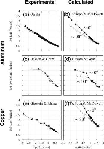The $E/\theta -\log \theta$ plot of the experimental data for the Al $〈100〉$ symmetric tilt boundary energy [5] is shown in Figure 1(a). As the plot is obtained by folding at 45${}^{\circ }$, the linear dependence on θ is observed not only near 0${}^{\circ }$ and 90${}^{\circ }$, but also at intermediate angles. The plot shows identical slopes for the experimental values, unlike those of the theoretical predictions. However, the EAM-calculated results [4] in Figure 1(b) show a lower slope angle for ${90}^{\circ }$ than for $0^{\circ }$, consistent with the Burgers vector dependency. This discrepancy, called Otsuki's dilemma, is observed in both experimental and calculated results [6] for Al (Figure 1(c,d)), as well as experimental [7] and calculated [4] results for Cu (Figure 1(e,f)). The discrepancy of the θ dependency between the experimental and calculated results may indicate a limitation in dislocation theory for predicting small-angle boundary energies.

Figure 1. $E/\theta -\log \theta$ plots of experimental and calculated results for Al and Cu.

These calculated results were obtained using empirical potentials of EAM [4] and Morse [6]. Studies of the boundary energy using empirical potentials have recently shifted in focus from the early stages of the investigations of structure and energy [8, 9] to the atomic-level dynamics. However, doubt remains regarding the stable structure or minimum energy of the grain boundary. Many calculations have been performed to confirm the consistency of the energy and structure, using the famous Large-scale Atomic/Molecular Massively Parallel Simulator (LAMMPS) to construct a database of calculated values [10, 11]. For obtaining more reliable energy values, the first-principles (FP) calculations have been performed [12–14]. The structure, energy, and more recently, the local stresses have been analysed using the FP method [15]. These results, including those reported in the author's preliminary work [16], are calculated for the ground-state energies and structures.

FP calculations may be appropriate for obtaining reliable boundary energies but may be unsuitable for comparing the finite-temperature energies of Otsuki's experimental results obtained at thermal equilibrium conditions of 513 K [5]. In Sutton and Balluffi [17], finite-temperature calculations of the boundary energy were only introduced for Au twist boundaries [18, 19]. Najafabadi et al. applied the local harmonic method and reproduced the experimentally observed drop in boundary energy with the temperature. They noted the linear dependence of the boundary energy on the excess volume. The entropic effects of the excess volume were first reported by Hashimoto et al. [8], who concluded that a pentagonal bipyramid existing on the consistent boundary was the main contributor to the excess entropy. Foiles revisited the temperature dependence of the grain-boundary free energy and estimated it using the temperature dependence of the material's elastic constants [20, 21]. However, these calculations were performed using only harmonic approximations with empirical potentials.

To include anharmonic effects in the FP calculations, Neugebauer's group recently proposed the method of up-sampled thermodynamic integration using Langevin dynamics (UP–TILD), which has been applied to systems [22, 23] that include stacking faults [24], but not to those with grain boundaries. The suitability of the key method of thermodynamic integration (TI) for grain boundaries was proposed by Frenkel and Ladd [25]. This method is still in extensive use with revisions and modifications [26, 27]. Very recently, however, Ganguly and Horbach noted the limits of the Frenkel–Ladd method and proposed a new approach that incorporated the roughening effect on the boundary energy [28] using the Lennard–Jones potential. FP calculations have not yet been applied to the finite-temperature grain-boundary energy.

In this research, FP calculations were performed for the Al $〈100〉$ symmetric tilt grain-boundary energies to obtain more reliable defect energies. The determined finite-temperature behaviour was compared with the experimental results obtained by Otsuki [3, 5]. First, we adapted the Boettger method, which provides reliable absolute ground-state energies for systems with alternating atom sizes [29]. Second, we also performed Einstein-model calculations of harmonic oscillators [30] and used the simple TI method proposed by Frenkel [31] to include anharmonic effects; the similarity between the Einstein system and the FP system limits the number of Monte-Carlo(MC) simulation steps expected following Bennett's recipe [32]. By this approach, we avoided the highly technical procedure of empirical potential fitting. Finally, we investigated the anharmonic contributions based on simple harmonic oscillations.

2. Computational details

The FP calculations were performed using VASP (Vienna ab initio simulation package) [33]. For the pseudopotentials of Al, we used the projector-augmented wave (PAW) method [34] and generalised-gradient approximation (GGA) [35]. The cut-off energy of the plane wave was the default of the potential. The total energies were obtained by the tetrahedron method, and the relaxations were performed by the Methfessel-Paxton method with order 1 [36]. The k-point meshes, which change with the unit cell's outer dimensions depending on the tilt angle θ, were provided by the automatic generator implemented in VASP. After we investigated the energy convergence as a function of the length parameter of the k-point mesh generator, fixed calculations were performed using the length parameter of 100. Ionic relaxations and finite-temperature calculations were performed using the length parameter of 50; this reduction decreased the VASP calculation time.

The unit cell models of the Al $〈100〉$ symmetric tilt boundary were prepared for $n_{\theta }=3$, 5, 7, 9, 11, and 13 with $\theta =\arctan \left(1/n_{\theta }\right)\times 2$ for angles near $0^{\circ }$, and ${90}^{\circ }-\arctan \left(1/n_{\theta }\right)\times 2$ for angles near ${90}^{\circ }$, corresponding to $\mathrm{\Sigma }=5$, 13, 25, 31, 61, and 85. Hereafter, each model is tagged following the scheme 0_3_16, which indicates the model for the $0^{\circ }$ side of $n_{\theta }=3$ with the system size of 16. Before relaxation, some atoms too near the boundaries were deleted; their effects on the boundary energies are detailed in the next section. The samples used for ground-state calculations are summarised in Table 1 with the system sizes. The relaxed atomistic configurations are shown in Figure 2, where (a) and (b) depict 0_11_224 and 90_11_468, respectively. To distinguish the atom configurations around dislocations, the unit cells are expanded in the xy directions. The central high-contrast rectangular region represents a unit cell, and the two boundaries are indicated by arrows. For the z-direction, two layers are supplied, as marked by open and closed circles. In the relaxed configurations, the structural units at the boundaries are identical to those obtained by Tschopp and McDowell [4]. The dislocation cores in the near-0${}^{\circ }$ models are pentagonal bipyramids, as previously reported [8].

Figure 2. Top views of the boundary models of 0_11_224 and 90_11_468.

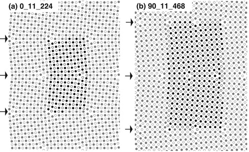
Table 1. Summary of boundary models for the calculations.

Model	$n_{\theta }$	Σ	θ [${}^{\circ }$]	Size of ground-states calc.	Size of Einstein calc.
0_3	3	5	36.87	16
0_5	5	13	22.62	34–94	40
0_7	7	25	16.26	88	88
0_9	9	31	12.68	148,152
0_11	11	61	10.39	220,224,228	92
0_13	13	85	8.80	312,316
90_3	3	5	53.14	36
90_5	5	13	67.38	96	56
90_7	7	25	73.74	188	88
90_9	9	31	77.32	312
90_11	11	61	79.61	468	92
90_13	13	85	81.20	656

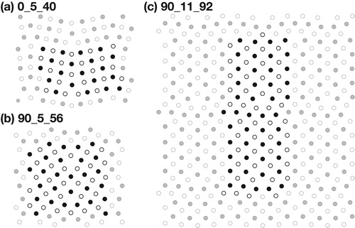
The models used for the Einstein calculations are reduced in system size and prepared as shown for 0_11_92 in Figure 3, where (a) shows the deletions of perfect regions and excessively close regions, and (b) and (c) show the models before and after their relaxations, respectively. The atom numbers are reduced from 224 to 92 for the Einstein calculations. The other models for the Einstein calculations are prepared in the same way. The relaxed configurations for 0_5_40, 90_5_56, and 90_11_92 are shown in Figure 4. The Frenkel calculations were performed on 0_5_40 and 90_5_56.

Figure 3. Deleting atoms of 0_11_92 for the Einstein calculations: (a) before deletion, and (b) before and (c) after relaxation.

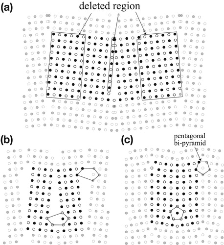
Figure 4. Relaxed configurations for (a) 0_5_40, (b) 90_5_56, and (c) 90_11_92.

3. Results

3.1. Ground-state calculation

The defect energy $\mathrm{d}E$ is obtained as the difference between the perfect lattice energy $E_0$ and the defect system energy $E_{\mathrm{d}}\left(n\right)$ $\mathrm{d}E=E_{\mathrm{d}}\left(n\right)-n{E}_0,$where n is the system size. The boundary energy is obtained by $\mathrm{d}E/A$ with the surface area A. The total energy convergences of the perfect lattice on the length parameters of the k-point meshes are shown in Figure 5. Because the break condition of the electronic self-consistent loop is ${10}^{-4}$ eV, the truncation errors are too small to observe in the figure. Although the energy per atom is scattered around 0.005 eV/atom for the length of 50, the convergency values are less than 0.0002 eV/atom for the lengths of 100 or more. However, the converged values are not identical.

Figure 5. Dependency of the energy per atom on the length parameter for different perfect models. Reference system model shapes are indicated by the unit cell sizes as $2\times 1\times 1$; system sizes are given in the parentheses.

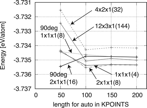
The model shapes of the reference systems are indicated by the unit cell sizes as $2\times 1\times 1$, with system sizes given in the parentheses. Two models of $2\times 1\times 1$ and $1\times 1\times 1$ near 90${}^{\circ }$ show similar values of −3.73474 and −3.73477 eV/atom, respectively. Meanwhile, three models of $1\times 1\times 1$ (4), $4\times 2\times 1$ (32), and $12\times 3\times 1$ (144) near 0${}^{\circ }$ show those of −3.73538, −3.73429, and −3.73508 eV/atom, respectively, with maximum differences of 0.001 eV. Because the unit cells for the boundary model include 100 atoms and more, these differences are not negligible.

The boundary energies with alternating unit cells vary with the reference energies $E_0$ of the perfect lattices. Figure 6 shows the dependency of $E_0$ on identical $n_{\theta }=5$ models near $0^{\circ }$ for system sizes of 34–94. With the reference of the $1\times 1\times 1$ cubic system, the energies are converge at approximately 510 mJ/m${}^2$. However, for that of the $4\times 2\times 1$ slab system, convergence occurs at approximately 490 mJ/m${}^2$ and the convergence value continues decreasing for system sizes larger than 94. For a larger perfect slab $12\times 3\times 1$, the convergence values are between these values. For the FP reference system, we use a perfect model with a k-point mesh similar to that of the defect system. Defect systems with irregular dimensions can be difficult to model via perfect lattices, Typical cases include surface models, but these are well addressed by Boettger's method [29].

Figure 6. Boundary energies predicted for different n−m numbers via Boettger method.

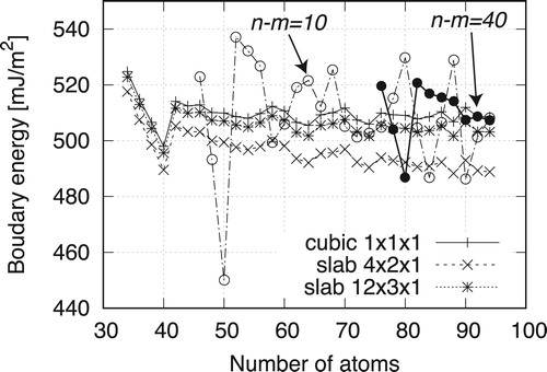
Boettger proposed the following equation: $\mathrm{d}E=E_{\mathrm{d}}\left(n\right)-n{E}_0=E_{\mathrm{d}}\left(n\right)-n\frac{E_{\mathrm{d}}\left(n\right)-E_{\mathrm{d}}\left(m\right)}{n-m},$where $E_0$ is supplied from the perfect region between the boundaries of the differently sized models. The plots for n−m=10 and 40 in Figure 6 show the converged boundary energies. The converged value is equal to that using the energy of the perfect $1\times 1\times 1$ cubic or $12\times 3\times 1$ slab model.

The Boettger method is computationally expensive for the FP calculations, so it is not used for the other boundary models. The consequent ground-state boundary energies, calculated with the reference value of the $12\times 3\times 1$ slab model, are shown in Figure 7. Values indicated by Einstein and Frenkel are obtained later. The energies are near those obtained by EAM. The boundary energies with $n_{\theta }=3$ and 5, an intermediate region, are about 500 mJ/m${}^2$, significantly higher than the experimental values, and the tangent angle near 0${}^{\circ }$ is larger than that near 90${}^{\circ }$.

Figure 7. Ground-state and finite-temperature boundary energies, obtained by the FP, Einstein model, and Frenkel methods, with EAM [4] and experimental [3] values, of the Al $〈100〉$ symmetric tilt boundary.

3.2. Harmonic Einstein model

The Einstein model gives the finite-temperature Helmholtz free energy of site i, $F_i(T,a)$, as follows: $F_i(T,a)=E_i^0\left(a\right)-k_{\mathrm{B}}T\sum _{j=x,y,z}\ln \left(\frac{\exp (-{\mathrm{\Theta }}_{ij}/2T)}{1-\exp (-{\mathrm{\Theta }}_{ij}/T)}\right)$where $E_i^0\left(a\right)$ is the lattice constant $a$ dependent on-site energy, ${\mathrm{\Theta }}_{ij}$ is the Einstein temperature of the j-direction on the i-site, given by $h{\nu }_{ij}\left(a\right)/k_{\mathrm{B}}$, and $k_{\mathrm{B}}$ and h are the Boltzmann and Planck constants, respectively. The total energy is obtained by the summation of $F_i$. The frequency ${\nu }_{ij}$ is obtained by ${\nu }_{ij}=\frac{1}{2\pi }\sqrt{\frac{k_{ij}}{m}}$where $k_{ij}$ is the spring constant and m is the weight of the oscillator, here equal to the atomic weight [37]. Each spring constant can be obtained by fitting to the total energies, with slight deviations in the j-direction on the i-site from the stable position.

We use the procedure of the free-energy calculation of the perfect lattice as an example. The lattice size is $2\times 2\times 2$ with 32 atoms. The temperature effect is included explicitly in the free-energy equation, and included implicitly via the lattice constant due to the thermal expansion. The lattice constant change affects the spring constant and the on-site energy $E_i^0$, as shown in Figure 8(a). The spring constant decreases drastically with increasing lattice constant. The on-site energy varies with the lattice constant, as shown in the right panel of Figure 8(a), which is equivalent to the $E-a$ curve. The lattice constant dependency of the free energy per atom is shown in Figure 8(b). Taking the minimum of each temperature curve, we obtain the thermal expansion curve of Figure 8(c).

Figure 8. Fitting procedures, Helmholtz free-energy surface, and thermal expansion by the Einstein model for a perfect fcc lattice.

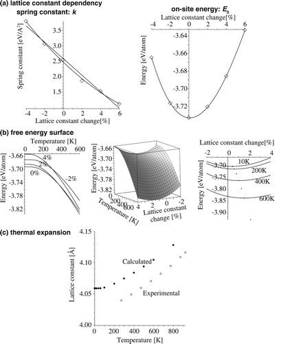
The thermal expansion obtained by the Einstein calculation shows a discrepancy compared to the experimental value, which is a well-known systematic bias of the local-density approximation (LDA) or GGA in the FP calculation. The reproduced linear thermal expansion coefficient is similar to those obtained by phonon calculations [38]. The Einstein temperature is linked to the free energy contribution. The lattice constant expansion at 300 K is 0.8155%, and the spring constant is 2.1391 eV/Å${}^2$. The frequency and Einstein temperature calculated from this are $\nu =6.225\times {10}^{12}$ Hz and ${\mathrm{\Theta }}_{ij}=298.8$ K, respectively. The latter is consistent with the experimental values of 284 K or 306 K [39].

As shown in the Boettger method in Figure 6, the small-size model reproduces a boundary energy similar to those produced by the larger-size models. Figure 9 (a) shows the relaxed atomistic configurations of 0_5_40. Arrows indicate the dislocation cores, which are the pentagonal bipyramid sites cited by Hashimoto et al. [8] Figure 9(b) shows examples of energy changes with deviations in the fitting of the spring constants of such sites. The upper panel is the case for a z-direction change with the lattice constant change of $-2$%, and its calculated points lie on the fitting curve of a second-order polynomial. The other directions of the other sites show different values but good fittings. For the lattice constant change of 0%, the fitting on the x-direction of this site is poor, but the discrepancy appears to be small at this scale. For the lattice constant expansion of 4%, however, typical anharmonic behaviour is observed on the same site and direction.

Figure 9. Fluctuation of each site predicted by the Einstein model, and the fittings of spring constants for 0_5_40.

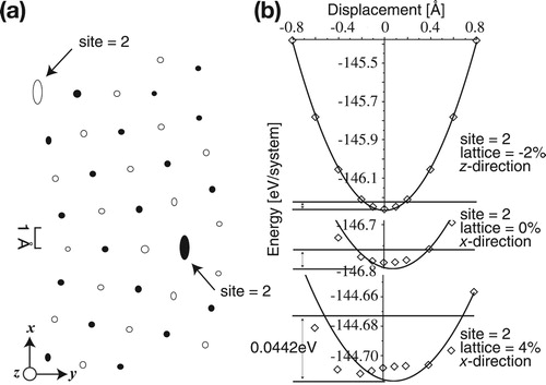
With the energy maximum of 0.044 eV, equivalent to 513 K, the fluctuating regions of all sites are illustrated in Figure 9(a). The central sites of the pentagonal bipyramids show large anharmonic fluctuations with amplitudes of about 0.7 Å in the x-direction. Only the right and left sites in the pentagonal bipyramid show slightly elliptical shapes. The total free energy of the boundary model is calculated by the summation of energies determined by the spring constants and the ground-state energy for different lattice constants. Some of the anharmonic sites discussed in Figure 9 are also fitted to the second-order curves.

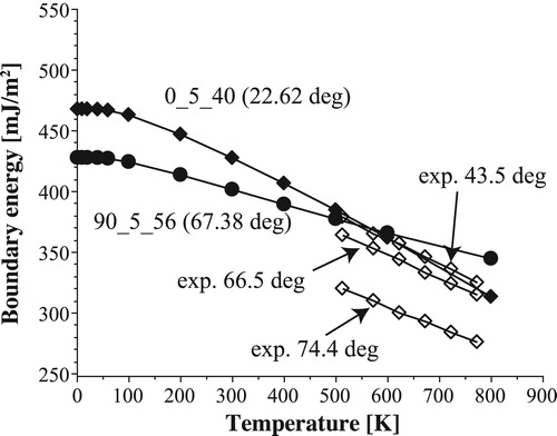
Figure 10 shows the temperature dependence of the boundary energies for 0_5_40 and 90_5_56, as well as those of the experimental results [3]. The absolute values of the calculated results are almost consistent with the experimental results. The temperature dependencies, however, show critical differences. The drops between 0 K and 500 K are 86 mJ/m${}^2$ near 0${}^{\circ }$ and 70 mJ/m${}^2$ near 90${}^{\circ }$. Without giving the results explicitly, the calculated results of the smaller-angle models show the same tendency. Consequently, the boundary energies near 0${}^{\circ }$ are close to those near 90${}^{\circ }$.

Figure 10. Temperature dependency of the boundary energy predicted by the Einstein model for 0_5_40 and 90_5_56.

The strong temperature dependence of the boundary energy and the differences in the models for 0${}^{\circ }$ and 90${}^{\circ }$ can be intuitively understood by the dispersion of the spring constants. Figure 11 compares three dispersion curves of the spring constants for the perfect fcc crystal and two boundary models. The curves are constructed by the sorted spring constants for the x,y,z directions of all sites. Because of the differences in system size, the x-axis is normalised by the system size times three. The y-axis shows the Einstein temperature calculated from the spring constant.

Figure 11. Dispersion of the Einstein temperatures of all directions of all sites. Inset: original spring constants, directions, and sites.

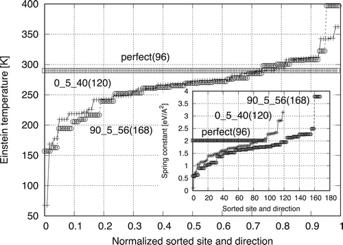
The perfect lattice shows an identical spring constant of 2.0156 eV/Å${}^2$ = 290 K for all directions of all sites. The value is smaller than that predicted at 300 K because of the thermal expansion and the decrease of the spring constant. The overall tendencies of the boundary models are similar near 0${}^{\circ }$ and 90${}^{\circ }$. In the middle range, the boundary models show more spring constants that are smaller than those of the perfect lattice. These smaller spring constants indicate that the free energy is lower than that of the perfect lattice, thus corresponding to higher stability. This is the main factor contributing to the decreasing temperature dependence of the boundary energy. As reported by Najafabadi et al. and Foiles [19, 20], the excess free volume and elastic constants are the main contributors to the finite-temperature boundary energy, which can be understood more quantitatively from the perspective of the spring constant distribution. At the grain boundary, the existence of dislocations increases the ground-state energy, but decreases the spring constants. Thus, the fluctuation areas increase, which increases entropy, and thereby the temperature dependence of the boundary energy is decreased.

In order to understand the different temperature dependences for the 0 and 90${}^{\circ }$ models, we study the details of the dispersion curve. The minimum spring constants appear at 67 K for 0${}^{\circ }$ and 157 K for 90${}^{\circ }$. The free-energy contribution at 513 K is $-0.0981$ eV for the perfect lattice, but $-0.1610$ eV and $-0.1246$ eV for 0 and 90${}^{\circ }$, respectively. Meanwhile, the maximum spring constants are present at 362 K and 397 K for 0 and 90${}^{\circ }$, with similar free-energy contributions of $-0.08852$ eV and $-0.08845$ eV, respectively. The minimum values of the 0${}^{\circ }$ model are obtained from the central sites of the pentagonal bipyramids as in Figure 9. Because the spring constants are forced to fit a second-order polynomial, low spring constants contribute to large free-energy drops, as reported elsewhere [8].

On the dispersion of spring constants, it is observed that the spring constants of the boundary sites are mostly different from those in the perfect lattice sites. There are two possible reasons for this: the size and the lattice constants of the boundary model. The former, the size of the model used in the research, was reviewed mainly in terms of energy convergence, but to achieve stress convergence, an increased size may be necessary. The latter, the lattice constants of the boundary model, were determined to be equal to the lattice expansion of the perfect lattice. More precisely, the lattice constants should be equat to the minimum Einstein free energy with the outer dimensions dependending on the spring constants. If the lattice constants of the boundary model are decreased, the spring constants are increased, and the dispersion curve remains in the plateau region. Higher-cost calculations are necessary to reveal the mechanism underlying this discrepancy.

The finite-temperature boundary energies with the Einstein model for $n_{\theta }=5$, 7, and 11 are added in Figure 7. The Einstein calculations at 1 K deviate from the ground-state calculations because of the zero-temperature oscillation and the lattice contants change. The points labelled as Frenkel are obtained later. The boundary energy at 513 K is similar to the experimental values from 250 to 350 mJ/m${}^2$. The energies for the small-tilt angles near 0${}^{\circ }$ and 90${}^{\circ }$ are similar, and the curve of the tilt-angle dependency becomes symmetric.

3.3. Anharmonic Monte-Carlo simulation

For the MC simulations, the system scaling factor, which determines the lattice constants, is fixed at 101.3268%, as obtained by the thermal expansion of the Einstein perfect lattice at 513 K. The Metropolis algorithm was performed in the MC simulation with a total energy equal to the linear combination of the target and Einstein energies: $E^{\mathrm{t}\mathrm{o}\mathrm{t}\mathrm{a}\mathrm{l}}=\lambda E^{\mathrm{t}\mathrm{a}\mathrm{r}\mathrm{g}\mathrm{e}\mathrm{t}}+(1-\lambda )E^{\mathrm{E}\mathrm{i}\mathrm{n}\mathrm{s}\mathrm{t}\mathrm{e}\mathrm{i}\mathrm{n}},$where the target system is expected to behave anharmonically with the energy obtained by FP. The anharmonic free energy is obtained by the TI of $F^{\mathrm{t}\mathrm{a}\mathrm{r}\mathrm{g}\mathrm{e}\mathrm{t}}=F^{\mathrm{E}\mathrm{i}\mathrm{n}\mathrm{s}\mathrm{t}\mathrm{e}\mathrm{i}\mathrm{n}}+{\int }_0^1〈\frac{\mathrm{d}{E}^{\mathrm{t}\mathrm{o}\mathrm{t}\mathrm{a}\mathrm{l}}}{\mathrm{d}\lambda }〉\mathrm{d}\lambda ,$with the integrand of $〈\frac{\mathrm{d}{E}^{\mathrm{t}\mathrm{o}\mathrm{t}\mathrm{a}\mathrm{l}}}{\mathrm{d}\lambda }〉=〈E^{\mathrm{t}\mathrm{a}\mathrm{r}\mathrm{g}\mathrm{e}\mathrm{t}}-E^{\mathrm{E}\mathrm{i}\mathrm{n}\mathrm{s}\mathrm{t}\mathrm{e}\mathrm{i}\mathrm{n}}〉,$where $E^{\mathrm{t}\mathrm{a}\mathrm{r}\mathrm{g}\mathrm{e}\mathrm{t}}-E^{\mathrm{E}\mathrm{i}\mathrm{n}\mathrm{s}\mathrm{t}\mathrm{e}\mathrm{i}\mathrm{n}}$ are recorded during the MC simulation.

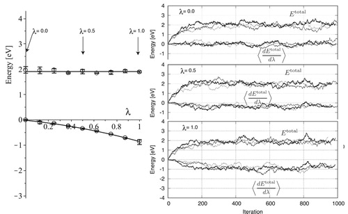
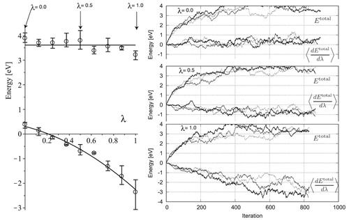
The example of the evolution of the total energy, $E^{\mathrm{t}\mathrm{o}\mathrm{t}\mathrm{a}\mathrm{l}}$, and its derivative of λ, $\mathrm{d}E/\mathrm{d}\lambda$, for the different λ values, are shown in the right column of Figure 12 for a perfect fcc lattice with the size of 32. The trial number of MC steps is 2000. At each step, all atoms move simultaneously, and the total energy of the system is calculated by VASP. The maximum atom movement is determined by the acceptance ratio of approximately 0.5. In performing MC at $\lambda =1.0$, representing a pure anharmonic system with no constraint at the Einstein position, the whole system drifts and $〈\mathrm{d}E/\mathrm{d}\lambda 〉$ becomes negatively large. As suggested by Frenkel and Ladd, we adopted the centre-of-mass fixing system [25, 40]. The drift contribution to the free energy is neglected because of the cancellation between the perfect and boundary models. Seeing $E^{\mathrm{t}\mathrm{o}\mathrm{t}\mathrm{a}\mathrm{l}}$, each system reaches thermal equilibrium after 2–300 MC steps. Each value of $〈\mathrm{d}E/\mathrm{d}\lambda 〉$ used in the λ integration is sampled from the iterations after 500 steps. Three different MC simulations are performed for a specific λ with different random-number seeds. The average, maximum, and minimum values are plotted in the left panel of Figure 12. The integrand is smooth and the dispersion of the values is small even at $\lambda =1$. The integrals are taken by the closed Newton–Cotes formula with nine nodes. The free energy calculated from the Frenkel method is low at 0.377 eV per system.

Figure 12. Frenkel simulation of perfect fcc lattice with the system size of 32.

Although the anharmonic contribution to the free energy per atom is as small as 0.01 eV, the anharmonic contribution to the boundary energy cannot be determined from this value, because the boundary energy is calculated by the difference in total free energies between the boundary and perfect lattices. Thus, we performed the same simulations on the boundary models of 0_5_40 and 90_5_56, as shown in Figures 13 and 14.

Figure 13. Frenkel simulation of boundary model of 0_5_40.

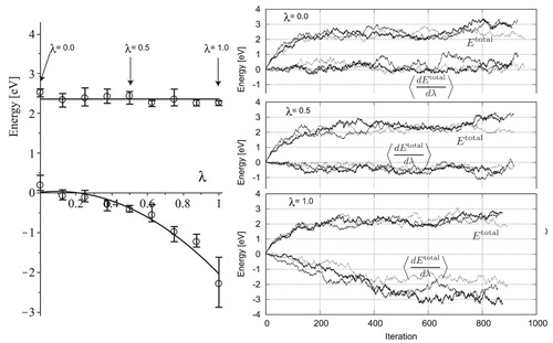
Figure 14. Frenkel simulation of boundary model of 90_5_56.

The average, maximum, and minimum values are plotted in the left panel of Figure 13 for 0_5_40 model. The Gibbs–Bogoliubov inequality, by which $〈{\mathrm{d}}^{2}E/\mathrm{d}{\lambda }^2〉$ is constrained to negative values or $〈\mathrm{d}E/\mathrm{d}\lambda 〉$ is decreased monotonically with λ [40, p. 171], is maintained; this is a simple proof of the validity of the simulation results. The large fluctuation observed at $\lambda =1$ affects the final integrated values with the deviation of 0.215 eV.

The integrand $〈\mathrm{d}E/\mathrm{d}\lambda 〉$ of 90_5_56 shows behaviour similar to that of 0_5_40 as depicted in Figure 14. Because this system includes more atoms and lower acceptance ratios, the maximum atom movement was set to a 10% decrease. The final integrated values are less dispersed in the range of 0.123 eV, even with the large fluctuation at $\lambda =1$.

The contributions of the Einstein model and the Frenkel simulation are summarised in Table 2. These energies are normalised by the number of atoms included in each system, as noted by $r_{\mathrm{a}\mathrm{t}\mathrm{o}\mathrm{m}}$. Using these values, the final results are predicted as follows: $\begin{array}{r}\mathrm{d}E=(F_{\mathrm{b}\mathrm{o}\mathrm{u}\mathrm{n}\mathrm{d}\mathrm{a}\mathrm{r}\mathrm{y}}^{\mathrm{E}\mathrm{i}\mathrm{n}\mathrm{s}\mathrm{t}\mathrm{e}\mathrm{i}\mathrm{n}}+F_{\mathrm{b}\mathrm{o}\mathrm{u}\mathrm{n}\mathrm{d}\mathrm{a}\mathrm{r}\mathrm{y}}^{\mathrm{F}\mathrm{r}\mathrm{e}\mathrm{n}\mathrm{k}\mathrm{e}\mathrm{l}})-r_{\mathrm{a}\mathrm{t}\mathrm{o}\mathrm{m}}\times (F_{\mathrm{p}\mathrm{e}\mathrm{r}\mathrm{f}\mathrm{e}\mathrm{c}\mathrm{t}}^{\mathrm{E}\mathrm{i}\mathrm{n}\mathrm{s}\mathrm{t}\mathrm{e}\mathrm{i}\mathrm{n}}+F_{\mathrm{p}\mathrm{e}\mathrm{r}\mathrm{f}\mathrm{e}\mathrm{c}\mathrm{t}}^{\mathrm{F}\mathrm{r}\mathrm{e}\mathrm{n}\mathrm{k}\mathrm{e}\mathrm{l}})\\ E_{\mathrm{b}\mathrm{o}\mathrm{u}\mathrm{n}\mathrm{d}\mathrm{a}\mathrm{r}\mathrm{y}}=\frac{\mathrm{d}E}{2A}\times 1.60218\times 10\times 1000\left[{\mathrm{m}\mathrm{J}/\mathrm{m}}^2\right]\end{array}$where $\mathrm{d}E$ is the free-energy difference between the boundary and the perfect models.

Table 2. Summary of the Einstein and Frenkel simulations [eV].

System	$n_{\mathrm{a}\mathrm{t}\mathrm{o}\mathrm{m}}$	$F^{\mathrm{E}\mathrm{i}\mathrm{n}\mathrm{s}\mathrm{t}\mathrm{e}\mathrm{i}\mathrm{n}}$	$F^{\mathrm{F}\mathrm{r}\mathrm{e}\mathrm{n}\mathrm{k}\mathrm{e}\mathrm{l}}$	$r_{\mathrm{a}\mathrm{t}\mathrm{o}\mathrm{m}}$	A(area) [Å${}^2$ ]
Perfect	32	$-121.56$	$-0.377\pm$ 0.033	–	–
0_5_40	40	$-149.90$	$-0.558\mp$ 0.215	40/32	42.99
90_5_56	56	$-210.03$	$-0.688\mp$ 0.123	56/32	60.46

The boundary energies determined using the Einstein model at 1 K and 513 K and by the Frenkel simulations are summarised in Table 3, as are the deviations of the integrated values for the anharmonic effects. Although Frenkel's results for the boundary energy near 0${}^{\circ }$ show large errors, the results remain near the experimental values in Figure 7. Thus, the anharmonic contributions to the boundary energies are smaller than the harmonic contributions for both the 0${}^{\circ }$ and 90${}^{\circ }$ models. The other boundary energies estimated by the Einstein approximation shown in Figure 7 are expected to be near those including anharmonic effects obtained with the Frenkel simulations.

Table 3. Calculated boundary energies [mJ/m${}^2$].

System	Einstein (at 1 K)	Einstein (at 513 K)	Frenkel
0_5_40	468	382	$366\pm 48$
90_5_56	428	358	$355\pm 24$

However, the Frenkel decrease of 0_5_40 is much larger than that of 90_5_56. The adopted initial state of the Einstein model includes ambiguity in the fitted curve for the anharmonic potential. Thus, the Frenkel results can be negative. Alternatively, the steep potentials observed in the dislocation cores may already include the anharmonic effects. Thus, the anharmonic contributions should be investigated further using more simulation steps with the high-precision VASP calculations.

4. Conclusions

Al $〈100〉$ symmetric tilt grain-boundary energies are obtained by the ground-state, harmonic, and anharmonic contributions, as determined by FP calculations. From the calculations, the following results are obtained:

• ground-state calculations The ground-state boundary energy obtained by the FP calculations is around 500 mJ/m${}^2$ for the random orientations. For smaller tilt angles, the obtained boundary energies exceed the experimental values, and the tangent angle near 0${}^{\circ }$ is larger than that near 90${}^{\circ }$. The Boettger method reveals that the small-size model reproduces a boundary energy similar to those produced by the larger-size models.

• harmonic Einstein model The finite-temperature effect predicted by harmonic oscillations of the Einstein model decreases the boundary energy relative to that of the ground state. The decrease for the boundaries with tilt angles near 0${}^{\circ }$ is larger than that for the boundaries with those near 90${}^{\circ }$. This is due to the large core of the dislocation, which is geometrically necessary to form a coherent small-angle boundary; this dislocation creates the difference in free energy decreases.

• anharmonic Monte-Carlo simulation The anharmonic effect predicted by the Frenkel method, using TI with MC simulations, shows a small contribution to the boundary energy. The consequent values are almost identical for the 0${}^{\circ }$ and 90${}^{\circ }$ models, and the energy curve is symmetric with the tilt angle. The calculated energies are consistent with previously reported experimental results.

Although our treatments of the finite-temperature calculations by FP are simple, these rough calculations reproduce reliable absolute values that are consistent with the experimental data. Such reliability and consistency demonstrate the necessity of more precise and higher-cost calculations.

The calculation method proposed in this paper can be applied to many defect types. The obtained results suggest limits on the ability of Burgers vector-based analysis to explain the finite-temperature behaviours of symmetric tilt grain boundaries. New approaches, including analyses of thermodynamic contributions, are expected to explain the behaviours driven by dislocation interactions.

Acknowledgments

This work was supported by JSPS KAKENHI Grant Number JP20K05067, and performed partially using the JFRS-1 supercomputer system at the Computational Simulation Centre of the International Fusion Energy Research Centre (IFERC-CSC) in the Rokkasho Fusion Institute of QST (Aomori, Japan).

Disclosure statement

No potential conflict of interest was reported by the author(s).

Additional information

Funding

This work was supported by Japan Society for the Promotion of Science (JSPS KAKENHI) Grant Number JP20K05067, and performed partially using the JFRS-1 supercomputer system at the Computational Simulation Centre of the International Fusion Energy Research Centre (IFERC-CSC) in the Rokkasho Fusion Institute of QST (Aomori, Japan).

References

- W. Shockley and W.T. Read, Quantitative predictions from dislocation models of crystal grain boundaries, Phys. Rev. 75 (1949), p. 692.
- W.T. Read and W. Shockley, Dislocation models of grain boundaries, in Imperfections in Nearly Perfect Crystals, W. Shockley, ed., chap. 13, John Wiley, New York, 1952, pp. 352–376.
- A. Otsuki, Research on boundary energy of Al, Ph.D. diss., Kyoto Univ., 1990, in Japanese.
- M.A. Tschopp and D.L. McDowell, Asymmetric tilt grain boundary structure and energy in copper and aluminium, Philos. Mag. 87 (2007), pp. 3871–3892.
- A. Otsuki, Energies of [001] small angle grain boundaries in aluminum, J. Mater. Sci. 40 (2005), pp. 3219–3223.
- G.C. Hasson and C. Goux, Interfacial energies of tilt boundaries in aluminium, experimental and theoretical determination, Scripta Metall. 5 (1971), pp. 889–894.
- N.A. Gjostein and F.N. Rhines, Absolute interfacial energies of [001] tilt and twist grain boundaries in copper, Acta Metall. 7 (1959), pp. 319–330.
- M. Hashimoto, Y. Ishida, R. Yamamoto, and M. Doyama, Thermodynamic properties of coincidence boundaries in aluminum, Acta Metall. 29 (1981), pp. 617–626.
- A.P. Sutton and V. Vitek, On the structure of tilt grain boundaries in cubic metals I. symmetrical tilt boundaries, Philos. Trans. R. Soc. A 309 (1983), pp. 1–36.
- M.A. Tschopp, S.P. Coleman, and D.L. McDowell, Symmetric and asymmetric tilt grain boundary structure and energy in Cu and Al (and transferability to other fcc metals), Integr. Mater. Manuf. Innov. 4 (2015), p. 11.
- E.A. Holm, D.L. Olmsted, and S.M. Foiles, Comparing grain boundary energies in face-centered cubic metals: Al, Au, Cu and Ni, Scr. Mater. 63 (2010), pp. 905–908.
- A.F. Wright and S.R. Atlas, Density-functional calculations for grain boundaries in aluminum, Phys. Rev. B 50 (1994-II), p. 15248.
- S. Ogata, H. Kitagawa, Y. Maegawa, and K. Saitoh, Ab-initio analysis of aluminum Σ=5 grain boundaries – fundamental structures and effects of silicon impurity, Comput. Mater. Sci. 7 (1997), pp. 271–278.
- T. Uesugi and K. Higashi, First-principles calculation of grain boundary energy and grain boundary excess free volume in aluminum: Role of grain boundary elastic energy, J. Mater. Sci. 46 (2011), pp. 4199–4205.
- H. Wang, M. Kohyama, S. Tanaka, and Y. Shiihara, Ab initio local energy and local stress: application to tilt and twist grain boundaries in Cu and Al, J. Phys.: Condens. Matter. 25 (2013), p. 305006.
- S.R. Nishitani, Energy of small angle tilt boundary in Al, in 10th International Conference on Processing and Manufacturing of Advanced Materials Processing, Fabrication, Properties, Applications (THERMEC), Materials Science Forum Vol. 941, Paris, France, 2018, pp. 2296–2299.
- A.P. Sutton and R.W. Balluffi, Interfaces in Crystalline Materials, Oxford Classic Texts in the Physical Sciences, Clarendon Press, Oxford, 1997.
- R. Najafabadi, D.J. Srolovitz, and R.A. LeSar, Finite temperature structure and thermodynamics of the Au Σ5 (001) twist bounday, J. Mater. Res. 5 (1990), pp. 2663–2676.
- R. Najafabadi, D.J. Srolovitz, and R. LeSar, Thermodynamic and structural properties of [001] twist boundaries in gold, J. Mater. Res. 6 (1991), pp. 999–1011.
- S.M. Foiles, Temperature dependence of grain boundary free energy and elastic constants, Scr. Mater.62 (2010), pp. 231–234.
- S.M. Foiles, Evaluation of harmonic methods for calculating the free energy of defects in solids, Phys. Rev. B 49 (1994), pp. 14930–14937.
- B. Grabowski, L. Ismer, T. Hickel, and J. Neugebauer, Ab initio up to the melting point: Anharmonicity and vacancies in aluminum, Phys. Rev. B 79 (2009), p. 134106.
- A.I. Duff, T. Davey, D. Korbmacher, A. Glensk, B. Grabowski, J. Neugebauer, and M.W. Finnis, Improved method of calculating ab initio high-temperature thermodynamic properties with application to ZrC, Phys. Rev. B 91 (2015), p. 214311.
- X. Zhang, B. Grabowski, F. Körmann, A.V. Ruban, Y. Gong, R.C. Reed, T. Hickel, and J. Neugebauer, Temperature dependence of the stacking-fault Gibbs energy for Al, Cu, and Ni, Phys. Rev. B 98 (2018), p. 224106.
- D. Frenkel and A.J. Ladd, New Monte Calro method to compute the free energy of arbitrary solids, application to the FCC and HCP phases of hard spheres, J. Chem. Phys. 81 (1984), pp. 3188–3193.
- J.M. Polson, E. Trizac, S. Pronk, and D. Frenkel, Finite-size corrections to the free energies of crystalline solids, J. Chem. Phys. 112 (2000), p. 5339.
- C. Vega and E.G. Noya, Revisiting the Frenkel-Ladd method to compute the free energy of solids: The Einstein molecule approach, J. Chem. Phys. 127 (2007), p. 154113.
- S. Ganguly and J. Horbach, Free energy of grain boundaries from atomistic computer simulation, Phys. Rev. E 98 (2018), p. 031301(R).
- J.C. Boettger, Nonconvergence of surface energies obtained from thin-film calculations, Phys. Rev. B49 (1994), pp. 16798–16800.
- A. Einstein, Die Plancksche Theorie der Strahlung und die Theorie der spezifischen Wärme, Ann. Phys. (Leipzig) 327 (1907), pp. 180–190.
- D. Frenkel, Free-energy computation and first-order phase transitions, in Molecular-Dynamics Simulation of Statistical-Mechanical Systems: Proceedings of the 97th International School of Physics “Enrico Fermi”, 1986, pp. 151–188.
- C.H. Bennett, Efficient estimation of free energy differences from Monte Carlo data, J. Comput. Phys.22 (1976), pp. 245–268.
- G. Kresse and J. Hafner, Ab initio molecular dynamics for liquid metals, Phys. Rev. B 47 (1993), pp. 558–561.
- G. Kresse and D. Joubert, From ultrasoft pseudopotentials to the projector augmented-wave method, Phys. Rev. B 59 (1999), pp. 1758–1775.
- J.P. Perdew and Y. Wang, Accurate and simple analytic representation of the electron-gas correlation energy, Phys. Rev. B 45 (1992), pp. 13244–13249.
- M. Methfessel and A.T. Paxton, High-precision sampling for Brillouin-zone integration in metals, Phys. Rev. B 40 (1989), pp. 3616–3621.
- M. de Podesta, Understanding the Properties of Matter, UCL Press, London, 1996.
- A.A. Quong and A.Y. Liu, First-principles calculations of the thermal expansion of metals, Phys. Rev. B 56 (1997-I), pp. 7767–7770.
- W. Mahmood, M.S. Anwar, and W. Zia, Experimental determination of heat capacities and their correlation with theoretical predictions, Am. J. Phys. 79 (2011), pp. 1099–1103.
- D. Frenkel and B. Smit, Understanding Molecular Simulation, From Algorithms to Applications, Academic Press, San Diego, 1996.