On the levelised cost of energy of windfarms

ABSTRACT

As windfarms spread, so have the discussions concerning their economics. Some argue from a basic definition of Levelised Cost of Energy (LCOE), that wind energy is more cost effective than other energy sources. The opponents argue that the LCOE must be estimated taking a systemic view including opportunity costs, which changes the picture. The opportunity costs are assessed in this paper using a novel approach based on a simulation model to estimate the number of windfarms that will achieve a certain nameplate output. Then, this is combined with the LCOE of dispatchable energy sources to estimate the opportunity cost. A Monte Carlo simulation is run to estimate the effects of uncertainty and variations. The results are clear – windfarms are not cost effective when a certain output must be guaranteed as major opportunity costs are introduced. However, as a supplementary source of energy in specific situations, windfarms can be useful.

KEYWORDS:

• Life-span
• Uncertainty
• Monte Carlo
• Opportunity cost
• El Hierro Island

1. Introduction

The pessimist complains about the wind; the optimist expects it to change; the realist adjusts the sails. William A. Ward

There is much debate among both laymen and academics, politicians and businesspeople as to how windfarms fare economically compared to traditional sources of energy. This is, of course, not just a question of costs but also of value. Despite the fact that an average American consumes 50 times more energy than an average Bangladeshi and 100 times more than an average Nigerian, relatively poorer villagers in Mali and Uganda are willing to pay about ten times higher price than the typical prevailing price in developed countries (Bazilian 2015). The villagers therefore place much more value for the same commodity, which shows that this is not just a question about costs. Indeed, the cost for an energy source can be the same mathematically while at the same time have very different net economic benefits. As Joskow (2011) puts it:

In a nutshell, electricity that can be supplied by a wind generator at a levelized cost of 6¢/KWh is not ‘cheap’ if the output is available primarily at night when the market value of electricity is only 2.5¢/KWh. Similarly, a combustion turbine with a low expected capacity factor and a levelized cost of 25¢/KWh is not necessarily ‘expensive’ if it can be called on reliably to supply electricity during all hours when the market price is greater than 25¢/KWh.

The value discussion is far too complex to address in a single paper as it depends on socioeconomic development of the region involved, alternative sources of energy, financial strengths, political processes, other local issues and more. Given this generic qualification, this paper aims at shedding light onto how to more correctly asses cost concerning windfarms on a conceptual level.

Crucial in this discussion is an approach called Levelised Cost Of Energy¹ (LCOE), whereby the total amount of power over the lifetime of an energy source is divided by the life cycle costs over the lifetime of the same energy source (Joskow 2011). The problem is that it (1) ignores the additional cost of integrating non-dispatchable energy sources into the grid, (2) the economic- and environmental externalities and (3) it has an implicit focus on new energy source development and not existing source generation (Benes and Augustin 2016). Additionally, LCOE ignores the value of the plant’s output to the grid (US EIA 2019).

For example, solar plants have much more attractive production profile relative to windfarms because society needs most of the energy during the day when the sun is shining whereas wind can come and go any time during the day. So, even though the LCOE of solar power is higher than wind energy it provides electricity that is more economically valuable (see Joskow 2011). Hence, ‘An LCOE comparison ignores the temporal heterogeneity of electricity and in particular the variability of VRE [Variable Renewable Energy]’ (Ueckerdt et al. 2013). Therefore, the true economics can be very different than the once predicated by the LCOE numbers.

Recognising this issue, there are many attempts at amending the cost calculation approach, as discussed in Section 2, but there are still serious issues left to solve. On top, we have subsidies and externality costs, such as the costs of carbon emissions, that make the calculations more difficult, and we can end up with value laden estimates disguised in economic numbers (Emblemsvåg 2016). Note that, the carbon pricing today is insufficient to make any real change. According to the World Bank Ball (2018), only four countries have priced carbon at or above the USD 40 floor – a floor set by the High-Level Commission on Carbon Prices, a group of leading economists, as a minimum price to achieve the emission cuts called for in the Paris climate accord.

Another issue often ignored is that when different technologies have different life-span the comparison can be difficult. Typically, a 20- or 30-year recovery period is chosen (see IRENA 2012; Stacy and Taylor 2019), but when the competing technologies last half a century or more, a simple, direct comparison is faulty as discussed later. Incredibly, the desire to actually use improved approaches is not there – not even adjusting the life span in the LCOE calculation to match the real life-span – in fact, Doemeland and Trevino (2014) state flat out that improved methods are not used in decision-making.

Therefore, whatever improvements are made concerning the cost of energy calculations, they should be as minimal as possible. This is an important criterium for this paper. Thus, entirely novel approaches such as Levelised Avoided Cost of Electricity (LACE), see for example, US EIA (2019), are not discussed in this paper. Rather, this paper addresses one of the most fundamental questions – the ‘opportunity cost’.² This cost is probably far greater than the differences produced by using different, refined approaches for calculating the LCOE of a windfarm.

Merriam-Webster defines opportunity cost as

the added cost of using resources (as for production or speculative investment) that is the difference between the actual value resulting from such use and that of an alternative (such as another use of the same resources or an investment of equal risk but greater return).

In our context, the alternative arises from the fact that windfarms will produce no energy at times, which requires a solution. This is evident from the simple fact that wind turbines typically start generating electricity at a wind speed of 3–5 m/s, reach maximum power at 11–12 m/s and generally cut out at a wind speed of around 25 m/s (IRENA 2018).

This gives two possible solutions – (1) accept blackouts or electricity rationing at times, or (2) have back-up energy supply that typically consists of dispatchable energy sources, improved grid management or trading over wider geographical areas. This gives basis for two research questions, that will be addressed in this paper:

1. Under what circumstances, if any, does LCOE provide a sufficiently correct cost estimate?

2. How can the LCOE including opportunity costs be estimated in a simple and robust way?

Note that ‘sufficiently correct’ is an important qualification. LCOE will by default never be correct if compared to reported annual cost accounts simply because the LCOE is a grand average. Actual costs will virtually always be over or below; an issue further exacerbated by the fact that the open domain data can be unreliable (Ederer 2015). Indeed, by using audited information from Special Purpose Vehicle companies – which many windfarms are defined in order to manage risks – Aldersey-Williams, Broadbent, and Strachan (2019) find an accurate way to calculate the LCOE for given years, which reveals that open domain data are unreliable. For example, they find that new wind farms are achieving a LCOE of around 100 GBP/MWh which is still considerably higher level than implied by the most recent CfD bids of 57.50 GBP/MWh.

Nevertheless, to find the answer to these research questions, we must first review the current approaches, as presented next. Then, in Section 3 a novel approach is presented through a simulation case, followed by a discussion in Section 4. Closure and future work are provided in Section 5.

2. Current approaches to calculating the cost of energy

The usage LCOE is widespread and used for policymaking worldwide (IRENA 2012) despite the acknowledged shortcomings of LCOE. For example, Stehly, Heimiller, and Scott (2017), on behalf of National Renewable Energy Laboratory, use representative utility-scale projects to estimate the LCOE for land-based and offshore wind power plants in the United States with no other alternatives explored. The same goes for Smart et al. (2016) in their project to provide the definition and rationale for the Baseline Offshore Wind Farm established within IEA Wind Task 26 – Cost of Wind Energy. This is sponsored by the International Energy Agency (IEA) Wind Implementing Agreement, an IEA Technology Collaboration Programme, for Co-operation in the Research, Development, and Deployment of Wind Energy Systems (IEA Wind). Both of these reports can therefore be viewed as the current state of the art at least concerning policymaking even though the opportunity cost, life-span and other issues are not discussed (see IRENA 2012; Smart et al. 2016; Stehly, Heimiller, and Scott 2017). Such costs are inherently ignored in the LCOE since the standard formula used for calculating the LCOE of renewable energy technologies is (IRENA 2012):(1) $\mathrm{L}\mathrm{C}\mathrm{O}\mathrm{E}=\frac{{\sum }_{t=1}^n{\displaystyle \frac{I_t+M_t+F_t}{{\left(1+r\right)}^t}}}{{\sum }_{t=1}^n{\displaystyle \frac{E_t}{{\left(1+r\right)}^t}}}$(1) Where LCOE, the average lifetime levelised cost of electricity generation; I_t, investment expenditures in the year t; M_t, operations and maintenance expenditures in the year t; F_t, fuel expenditures in the year t; E_t, electricity generation in the year t; r, discount rate; n, economic life of the system.

The numerator is essentially the Life-Cycle Cost (LCC) while the denominator is the discounted sum of energy/electricity generated over the life-cycle. Since the formula discounts both the numerator as well as the denominator, we end up with an undiscounted number, a point also discussed by Loewen (2019). If we simplify the formula and let the denominator basically become the sum of the energy produced, then LCOE becomes more logical and basically a life-span, grand average. Nevertheless, from mathematics we know that this masks the true variation, and this is where the opportunity cost issue comes in. Indeed, Joskow (2011) is one of the early to discuss the question of opportunity costs, and media such as The Economist (2014) picked it up later. However, there are still many unsolved issues concerning LCOE for windfarms.

First, it is important to recognise that LCOE can be calculates in various ways. For example, for offshore wind energy, two types of analysis are typically used (Smart et al. 2016):

1. A common cash flow model to explore the impact of market and policy factors on the delivered cost of offshore wind in each country under constant assumptions about baseline technology and site characteristics. The model used by Smart et al. (2016) is one developed by TKI (Top consortia for Knowledge and Innovation) in The Netherlands.

2. Bottom-up, engineering-based models (e.g. electrical infrastructure, O&M) under development by various countries can be verified, first by exercising the models to define baseline costs, and second, by conducting sensitivity analysis around the baseline project description by varying technology assumptions and site characteristics relative to the baseline technology description.

The same fundamental shortcomings persist. Hence, we need to look for new avenues to find better approaches. Indeed, several authors have found in diverse settings such as the UK, California and North-Western Europe that as the market share of VRE becomes large then the value drops rendering the LCOE useless for comparison (see Reichenberg et al. 2018; Ueckerdt et al. 2013) for more information.

Another shortcoming is that current LCOE calculations penalise established power plants (Stacy and Taylor 2019), and the ‘LCOE excessively penalises projects with longer expected lives and with higher discount rates’ (Loewen 2019). This is actually found to be true in real life also. By using the most recently available public data collected by the Federal Energy Regulatory Commission (FERC) in its Form 1 database to estimate LCOE-Existing, (Stacy and Taylor 2019) compare these estimates to the Department of Energy, Energy Information Administration’s (EIA’s) most recent estimates of LCOE (New Resources), adjusted for today’s fuel prices and capacity factors. From this they find that for all major dispatchable generation resources, the LCOE from new plants would on average be higher than the LCOE from existing resources, see Figure 1. Note that the data for existing solar- and wind power plants is too poor to be used, which is why they are not included in Figure 1.

Figure 1. LCOE from new and existing resources. Source: Stacy and Taylor (2019).

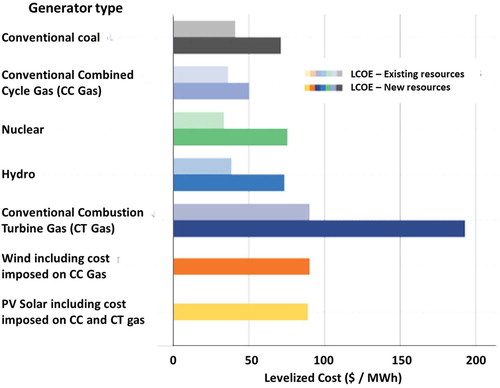
The reason for this penalty is that existing, dispatchable power plants have typically lower fixed costs than relatively new, or new, power plants, and dispatchable power plants have longer lives than the cost recovery period most LCOE calculations are based on. At a typical, existing power plant only the component need be replaced if it is worn out, and not the entire plant. Such replacements can continue indefinitely, in principle. When some of these plants have long lives after the typical 30 years used in LCOE calculations by US EIA (Stacy and Taylor 2019), the LCOE calculations do not provide the right picture concerning existing power plants.

The International Renewable Energy Agency (IRENA) is an intergovernmental organisation that aims at supporting countries in their transition to a sustainable energy future, but they ironically use even shorter recovery periods; a 20-year cost recovery period (IRENA 2012). This means that their analyses are skewed in favour of new technologies, and not longevity, and ignore the fact that a nuclear power plant, for example, has a regulatory end of life currently defined to be 60 years, but may be extended to 80 years.³ Similarly, hydro-electric power plants are on average 65 years old, and the oldest in the US are from 1891 (nine small power plants at 3.9 MW in total). In Table 1 we see the entire US portfolio of power plants. As we see, 30 years is too short life-span for most dispatchable technologies.

Table 1. Age, number of operational years and number of power plants per energy source 2019.^a

Energy source	Number of power plants		Operational years		Average age
C gas	1935	8.7%	3,870,188	8.7%	18.9
Coal	697	3.1%	1,376,642	3.1%	43.9
CT gas	2265	10.2%	4,519,846	10.2%	23.5
Hydro-electric	4190	18.8%	8,186,234	18.4%	65.2
Nuclear	97	0.4%	192,103	0.4%	38.6
Solar	3576	16.0%	7,205,477	16.2%	4.0
Wind	1342	6.0%	2,696,650	6.1%	9.6
Other gas	1876	8.4%	3,726,579	8.4%	32.6
Other	6337	28.4%	12,634,823	28.5%	25.2
Total	22,315	100.0%	44,408,542	100.0%	28.9

^aCalculated from US EIA Inventory of Operating Generators as of July 2019 found on https://www.eia.gov.

Basically, new technologies do not provide enough productivity gains to offset the advantage that existing power plants have concerning lower fixed costs (Stacy and Taylor 2019).

Many have realised the shortcomings of LCOE, but not amended it. In the literature, there are two main avenues of improving the LCOE – either refining the basic LCOE or create a System LCOE – as discussed subsequently.

2.1. Basic improvements of LCOE

There are many ways of improving the basic LCOE. One approach is to keep the LCOE but allow for price variations as discussed by Nissen and Harfst (2019). This will undoubtedly result is a more accurate estimate, but the fundamental issues persist.

A second improvement is to use reference scenarios and provide a comparative LCOE analysis (see Ebenhoch et al. 2015). This will eliminate the relative distortion as all cases are compared in the same way with the same methodological shortcomings. However, when absolute numbers are required this will not work. Furthermore, if the investment case is large enough to impact the market then it will also fail because the opportunity cost is ignored as well as the life-span issues.

A third approach of improvement is to explicitly model the uncertainty, as advocated by Ioannou, Angus, and Brennan (2017) amongst others. This is a basic requirement of any, realistic LCC approach (Emblemsvåg 2003), so it is remarkable that LCOE analyses are even conducted without. As Tran and Smith (2018) demonstrates, uncertainties in input data can significantly influence the LCOE values, which will also be demonstrated later in this paper. For renewables, this situation is exacerbated by both the lack of historical data and that renewable energy resources are geographically dependent (Tran and Smith 2017).

A fourth improvement is to include Power Purchase Agreements (PPA). Such agreements have become important in the US, for example, because renewable energy is more expensive and utilities have to buy certain amount of renewable energy according to the Renewable Portfolio Standards (RPS). Since buyers in the PPA can create terms that limit the annual purchase of energy, they therefore also affect the actual LCOE. This shortcoming can be amended, and (Bruck, Sandhorn, and Goudarzi 2018) show how.

Finally, we can take an investor’s view and assume investment positions and various ownership stakes through different phases of the life cycle of a windfarm (see Ioannou, Angus, and Brennan 2018). They find that the most important parameters on the NPV are not related to the cost-side of the case but to the revenue-side and the financial side. Specifically, the discounting factor, the energy price used in the model and the energy production are the three most important parameters overall. The latter two are a direct result of the issues discussed earlier – wind and market share. The results in this paper supports their findings.

The problem with these approaches – even if they were combined into one improved approach – is that the opportunity costs are ignored. One way to reduce this issue is to take a portfolio view whereby the lack of production from one windfarm is offset by the production from another. This makes sense not only because farm size matters, for example, Myhr et al. (2014) find that a significant increase in the number of turbines can give approximately 10% reduction in the LCOE, but also because many farms can have different weather conditions and a portfolio approach will reduce the weather risk. As will be shown in Section 3, this is crucial, but difficult to achieve. Another way is to create a Systems LCOE as discussed next.

2.2. Introducing system LCOE

An systems approach that does take a portfolio view is provided by Ueckerdt et al. (2013) as they present a System LCOE defined as the sum of their LCOE and the integration costs per unit VRE. Since there is no consensus on the definition of the integration cost (Milligan et al. 2011), the authors assert that the integration costs are all additional costs in the non-VRE of the power system when VRE are introduced, i.e. the opportunity cost as denoted in this paper. This cost is typically decomposed into three cost components – (1) balancing costs, (2) grid costs and (3) adequacy costs, or capacity costs. Balancing costs occur because VRE supply is uncertain. Grid costs occur as investments in transmission lines may be warranted and because the VRE output varies a lot – also upwards so there may be congestion costs. These costs are relatively direct in nature and therefore relatively easy to estimate and include into an opportunity cost estimate.

The adequacy costs, or capacity costs, traditionally reflect the cost of back-up capacity. This is, however, not the full picture so (Ueckerdt et al. 2013) correctly add the overproduction costs and full-load hour reduction costs to better reflect the adequacy costs – which they denote profile cost. The overproduction costs arise because the VRE results in producing energy when it is not needed due to its non-dispatchable nature, while the full-load hour reduction costs are caused by the average utilisation of the back-up energy sources falling as VREs are introduced. This profile cost is clearly an opportunity cost.

It should be noted that Ueckerdt et al. (2013) also discuss the flexibility costs associated with the dynamics of ramping up and down dispatchable energy sources in response to the variability of the VRE, but since this cost is negligible compared to the other costs (Hirst and Hild 2004), it is sensibly ignored for simplicity. Using these definitions, Ueckerdt et al. (2013) develop a set of equations that estimate the System LCOE. The result from their analysis is very interesting:

1. At moderate and higher wind market shares (>20%), marginal integration costs are in the same range as generation costs.

2. Integration costs significantly increases with growing market shares.

3. The profile costs are the largest market share of the integration costs.

4. Short-term System LCOE are larger than long-term System LCOE. This is due to capacity of dispatchable energy sources need time to adjust, i.e. reduce to account for the introduction of the VREs.

They also identify three integration options to reduce the System LCOE and hence reduce the economic barrier that items 1 through 3 above result in. The first option is to adjust the capacities in the grid to a mix with lower capital costs. The second is to increase transmission capacities – this reduces integration costs strongly, they assert. The thirds option is to shift demand or supply in time to better balance supply and demand something that can be achieved through storage or demand-side management.

Building upon this, Reichenberg et al. (2018) improve the approach further by adding trade- and storage capacities, and they study market share up to 100% – a level of market share they claim has not been studied before. Trade is especially important for VRE technologies, and in particular wind energy, since it enables variability smoothing (Mileva et al. 2016), and storage capacities is important for high market share (Jägemann et al. 2013).

Not surprisingly, with these refinements Reichenberg et al. (2018) obtain somewhat different results than (Ueckerdt et al. 2013). Noted shortcomings of the model from the authors is that (1) some technical aspects are not accounted for, (2) the power system currently in place is not accounted for, (3) transmission connections are limited to the necessary transmissions between large regions ignoring what is required within those regions, (4) the time resolutions is 3 h and not continuous and (5) the inter-annual variability of average wind speed is not accounted for. A sixth limitation could be added – the model formulation is linear.

Nevertheless, the model is a solid attempt at modelling the integration costs, which is nowhere in the literature well-defined (Ueckerdt et al. 2013). Furthermore, for a large electricity system such as the European one it is not obvious how to define the integration costs of VRE (Ueckerdt et al. 2013). With all the limitations such models inevitably will have, they find that the integration costs increase linearly up to market share of 80% after which there is a sharp increase in the integration costs.

It is clear that the modelling of Reichenberg et al. (2018), Ueckerdt et al. (2013) require major effort and is therefore not likely to take place in practice for most projects. However, they can serve well for policy making and the longer term since those decision-makers are more willing to spend the time and money for such a study. This said, there is a couple of assumptions in the modelling that is difficult to defend, which must be rectified for their models to be worth the effort of making them.

First, they assume that trade can essentially create a diversification situation in which windfarms can offset each other so that if one is not operational another one will be. This is difficult to argue since high-pressure weather systems can easily affect very large geographical areas such as western Europe and stop thousands of windfarms at the same time for days on end. With the increased volatility of the climate, this situation is more likely to occur more frequently in the future. In the next section, it will be shown how this assumption will fail. Second, and related to the first, storage is unlikely to handle the enormous volatility high market share of VRE over large geographical regions can create.

3. Calculating the opportunity cost of windfarms

Somewhere between 0% market share and 100% market share of wind energy, there will be a point where the true costs of windfarm energy start to deviate significantly from the LCOE. This is when wind energy impacts the grid enough to keep, or lower, the energy prices to such an extent that investments in dispatchable energy sources is being impacted. Thus, increasing market share of wind energy will over time result not necessarily in less output of energy but in a more volatile energy market with an increasing risk of energy shortage and a crowding-out of dispatchable energy sources resulting in an even higher volatility. Overall, the energy system will become more costly.

This occurs in real life where a significant amount of non-dispatchable energy resources have been added to the grid, see Figure 2. Here we see the ‘duck curve’ created by the solar energy entering the grid during a ‘typical spring day’ in California. Two major deviations from the average have been highlighted, which illustrates the amount of variation we are talking about.

Figure 2. The duck curve; typical load per the hour of a typical spring day in California in the 2010s. Source: CAISO (2016).

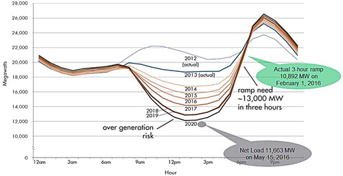
The cost of this ‘duck curve’ is substantial. Even with a market share as low as 1%–12%, the costs (imposed cost because it is due to Solar PV energy) fall in the range of 20–26 USD/MWh (Stacy and Taylor 2019), which compared to the LCOE in Figure 1 is roughly a 25% increase. This finding seems highly at odds with the doubling of the LCOE of non-dispatchable energy resources reported in the literature, see e.g. Reichenberg et al. (2018), as their market shares approach 100%.

Another example is the volatility in the German energy market, see Figure 3. The German VRE production was record-high in the first half of 2019 with a market share of 44% as stormy weather boosted wind power production on land and at sea, the utility association BDEW said.⁴ However, the daily fluctuations are enormous as Figure 3 shows. This is currently handled by trade, but what if all of Europe relied on wind energy?

Figure 3. 9 months daily production of renewable energy in Germany. Source: www.fraunhofer.de.

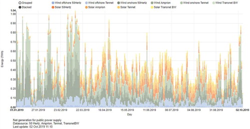
With just 13.6% of electricity in Europe being traded among countries (Batalla-Bejerano, Paniagua, and Trujillo-Baute 2019), a solution like this would not only require enormous investments in transmission capacity, but also major changes in regulatory work in all the impacted countries. It will also have major political consequences since this will result in price changes in various countries, production capacities and ultimately employment. This comes as a result from the finding that ‘ … 1% increase in the exporter’s electricity price reduces energy trade by an average of 0.7%, whereas a similar increase in the importer’s electricity price increases energy trade by an average of almost 1%' (Batalla-Bejerano, Paniagua, and Trujillo-Baute 2019). Overall, this seems to be a farfetched solution for decades to come even if it makes sense concerning the weather conditions.

To address this, we should ideally build a model of the grid, including all major energy generators, model the uncertainties in supply and demand, and estimate their impacts on prices and investments over decades. Naturally, as USDE (2015) also points out, this will vary significantly from area to area requiring detailed modelling. Such modelling would be a major undertaking far outside the scope of this paper, and it is to the knowledge of this author not undertaken by anybody so far. The impact on the LCOE will significant.

This paper therefore operates at a more conceptual level, and it aims to take an entirely different route than so far chosen in the literature as far as this author is aware. The approach is to model the LCOE of guaranteeing a certain nameplate output in total, and then run a simulation to assess the impact of the variations. In a sense, this approach includes trading explicitly into the model instead of assuming that it will fix itself. However, neither the costs of trading nor the required grid system is included. As such, the model is still a basic LCOE model similar to the ones discussed in Section 2.1. This means that the cost estimates will be understated to the true costs, i.e. the model is conservative. The US market is chosen due to the good data availability.

3.1. Capacity and windfarms

The vision of USDE (2015) is to increase wind as a source of electricity up to 35% in 2050. This means that they view wind energy as an addition to the current main sources, and not as a replacement of all fossil fuel sources since they foresee growth in energy demand. This seems to be sensible policy, and we can without further delay also conclude concerning RQ 1 that there are circumstances where LCOE does provide a sufficiently correct picture to be useful, and that is when the impact on the overall energy supply in the grid is negligible. This occurs in two possible cases. First, when VRE mostly provides auxiliary energy for example by providing energy for an industrial plant that has other energy solutions itself when wind energy is not available. Examples include the Nyhamna gas processing plant in Norway that wants to use a 350 MW offshore windfarm to boost power supply security (see Karagiannopoulos 2018).

Second, when VRE has negligible market share in the grid that it impacts neither energy prices nor the investment appetite (as it relates to price levels) concerning non-VRE energy sources. Several authors have found that when the market share of VRE becomes large the value drops (see Reichenberg et al. 2018; Ueckerdt et al. 2013) for more information. Understanding the market in each case is therefore important and to utilise various technologies to minimise the impact of the output variations from windfarms – specific cases require specific solutions.

The US electricity sector in 2019 was structured as shown in Table 3 with the respective LCOE from 2018. If we include Hydro-electric as a dispatchable energy source, the weighted average is 59.64 USD/MWh. We see that wind has a modest market share, but it is rising. The US EIA (2017) estimates that electricity use (sales plus direct use) will grow at an average of less than 1% per year to 2050. Since this change is slow and modest, it is no doubt that more competitive wind energy will result in lower prices, which in turn will result in less willingness to invest in other sources of energy which means that the structure of the energy market will change over time. In fact, about 83 GW of coal- and nuclear generation capacity have retired since 2011.⁵ The risk of energy shortages will therefore increase. The question is, how much volatility can wind energy bring into the energy market? It is beyond the scope of this paper to calculate this, but a simple illustration is provided later.

Another key parameter is the Power Capacity Factors (PCF). The improvements in technology and improved locations have given major improvements in PCF. The global weighted average PCF for onshore wind increased from around 20% in 1983 to around 29% in 2017 (a 45% improvement). Whereas the global the weighted average PCF for offshore wind increased even more (56%) from an even higher starting-point (IRENA 2018). Both onshore- and offshore windfarms have today about 42%–43% PCF on average but with large variations depending on location. For the purpose of this paper, 43% is used. Note that the nominal PCF can be well over 50%, but due to several types of losses it ends up about 10 percentage points lower (see Myhr et al. 2014).

A simple Monte Carlo simulation model is provided in Table 2 where the effects are calculated on a monthly basis for a windfarm for any given year, and they are calculated independently for all four farms (hence, four identical lines in the deterministic case). This is tantamount to assuming that the weather systems are random/independent towards these windfarms, which is an ideal case. Furthermore, the simulation should ideally have been on continuous basis, or at least hourly, but the data are missing for that purpose. The fact that a windfarm only produces energy 43% of the time globally, i.e. an Expected Capacity Factor (ECF) of 43%, and that historical Net Capacity Factors (NCF) have varied from about 25% to 55% for onshore windfarms and 32% to 55% for offshore windfarms in the US (Stehly, Heimiller, and Scott 2017), have huge impact on the opportunity costs.

Table 2. Simple Monte Carlo capacity simulation model on monthly basis.

Wind-farm	Year hours	ECF Jan	ECF Feb	ECF Mar	ECF Apr	ECF May	ECF Jun	ECF Jul	ECF Aug	ECF Sep	ECF Oct	ECF Nov	ECF Dec
1	8760	43%	43%	43%	43%	43%	43%	43%	43%	43%	43%	43%	43%
2	8760	43%	43%	43%	43%	43%	43%	43%	43%	43%	43%	43%	43%
3	8760	43%	43%	43%	43%	43%	43%	43%	43%	43%	43%	43%	43%
4	8760	43%	43%	43%	43%	43%	43%	43%	43%	43%	43%	43%	43%
Sum	Monthly average			730
Output coefficient						Min	1.72			Max	1.72
Wind-farm	Total hours	Jan	Feb	Mar	Apr	May	Jun	Jul	Aug	Sep	Oct	Nov	Dec
1	3767	314	314	314	314	314	314	314	314	314	314	314	314
2	3767	314	314	314	314	314	314	314	314	314	314	314	314
3	3767	314	314	314	314	314	314	314	314	314	314	314	314
4	3767	314	314	314	314	314	314	314	314	314	314	314	314
Sum	15,067	1256	1256	1256	1256	1256	1256	1256	1256	1256	1256	1256	1256
Output coefficient		1.72	1.72	1.72	1.72	1.72	1.72	1.72	1.72	1.72	1.72	1.72	1.72

The output coefficient in the model is the ratio between the number of hours with production per month compared to the total number of hours per month, i.e. 730 on average. So, a coefficient less than 1.00 means energy shortage. The maximum value indicates the best monthly ratio and the minimum value the lowest monthly ratio of the same windfarms. From Table 2 we see that deterministically speaking there is no difference. We also see that the four windfarms produce on average the output equivalent to 1.72 windfarms. In other words, four windfarms would have to trade between themselves to guarantee the output of less than 2. Furthermore, due to the weather conditions, these windfarms must be located far apart so that we can assume that the weather conditions are random towards each other.

Then we include uncertainty into the model. Triangular uncertainty distributions are used where NCF varies from 25% to 55% with an ECF of 43%. The model is subsequently run 50,000 times, and the results are shown in Figure 4.

Figure 4. Ratio of actual production output to full-time nominal output for three and four windfarms assuming uncorrelated weather.

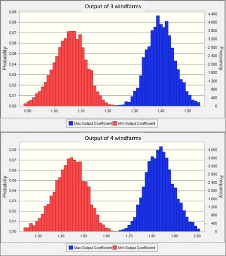
Surprisingly, perhaps, from the overlay chart to the left we find that we need four windfarms to guarantee the nominal (nameplate) output of one windfarm even under the assumption that the weather is not correlated. If we have only three windfarms, we see from the overlay chart to the right that there will be blackouts. More accurate analysis of the model reveals that with three windfarms there is 20% probability of blackouts. Trade is the solution to this according to many (see e.g. Mileva et al. 2016), but if large enough areas have high enough market share of wind and they are all being impacted by the same weather pattern, this problem is not going away as discussed earlier concerning trade in Europe.

Almost equally bad for the volatility of the energy prices, and hence investment appetite for other sources of energy, is that the production of energy will become 60% above nominal output. In short, three windfarms – each with a nominal output effect of 300 MWh – will produce anywhere from 0 to 480 MWh at random out of which 20% of the time the production is 0. From this we understand that as windfarms constitute an even larger portion of the energy supply of a country, the more volatile the prices will become and the duck curve in Figure 2 is instructive as is the situation in Germany shown in Figure 3.

We have so far only analysed the capacity aspect of windfarms. To understand what this means in economic terms, we need more information and this is discussed next.

3.2. The costs of windfarms

To build a simple model using publicly available information, we need installation costs, Operations & Maintenance (O&M) costs, life-span estimates, discounting factors, inflation estimates in addition to the capacity model just discussed. For simplicity, all other costs are ignored because they are very case specific, such as local grid costs, the distribution/transmission costs, the costs of frequency management, which is challenging with non-dispatchable energy resources (CAISO 2016), special environmental costs and more. These costs may also be partially included in the publicly available numbers. Thus, omitting them is best to avoid double-counting.

Since wind is a relatively new energy source the widest possible database is important for the model, and this is the IRENA (2018) database, which covers 85% of all onshore installations from 1983-2016. The fall of estimated global weighted average in total installed cost of onshore wind farms between 1983 and 2017 was 70%, as installation costs fell from USD 4880 to USD 1477 per kW. In our model, onshore costs of 1477 USD/kW are used. Since there is a significant spread, including uncertainty is crucial. Note that offshore windfarms are more expensive due to larger foundations, demanding location and more difficult grid connections (IRENA 2018). However, on average, offshore wind projects harvest more energy than onshore wind projects, notably in Europe, due to the better availability of wind resources, less turbulence and overall steadier winds. This has led to windfarms being placed further and further off shore with the result that the global weighted average installed costs increased by 4%, up from 4430 to 4487 USD/kW between 2010 and 2016 (IRENA 2018). However, despite technological improvements and greater output, offshore wind still constitutes a small portion of today’s global capacity. Offshore wind was 14 GW at the end of 2016, or just 3% of total installed wind capacity.

Concerning the O&M costs, MAKE Consulting (2017) finds that they ranged from 16 to 37 per USD per kW per year in 2016 in the United States, while the weighted average was 27 USD per kW per year. In our simple model, we therefore use 27 USD per kW per year. It should be noted that O&M costs are also higher for offshore wind because of the complexity of servicing offshore wind turbines due to the more challenging location requiring service ships, for example.

The opportunity cost can be readily estimated by using the LCOE of dispatchable energy sources with the assumption that we are ignoring the long-term effects of less investments and less capacity. We thereby ignore the crowding-out effect that the windfarms have on dispatchable energy sources due to the duck curve effect and its deepening. Since the dispatchable energy sources must exist to guarantee the energy output, we can calculate the weighted average LCOE for dispatchable energy sources in Table 3, which is 59.64 USD/MWh, and use that to calculate the opportunity cost. The model is therefore only capturing a given year, i.e. in the 2015–2019 range. Furthermore, the model is extrapolating the current situation into the future. This is simplistic, but sufficient to prove the point that the Total LCOE is much higher than most believe, and that the current calculation approach is highly distorted.

Table 3. US market share by capacity^a and LCOE.^b

Electricity sources	Market share by nameplate capacity	LCOE [USD/MWh]
CC gas	25.4%	46.30
Coal	21.3%	58.60
CT gas	12.8%	89.30
Hydro-electric	8.5%	39.10
Nuclear	8.6%	77.50
Solar	2.8%
Wind	8.3%
Other gas	7.4%
Other	4.9%
Sum	100.0%

^aMarket share are calculated from US EIA Inventory of Operating Generators as of July 2019 found on https://www.eia.gov.

^bCalculated by Stacy and Taylor (2019) using numbers from US EIA.

The resulting model is presented in Table 4, where the LCOE is calculated using Equation (1). The uncertainty is modelled as triangular distributions with the min-, average- and max values from US EIA (2019) except for the inflation, which is distributed as a normal distribution with an expected value of 2.5% and a standard deviation of 0.25%, and a discounting factor⁶ of 10% with 1% standard deviation. On average, these four windfarms will have an effect of 602 MW, or 5274 GWh/year.

Table 4. Estimating the LCOE of four onshore windfarms using 30 years life-span.

Wind-farm	Nominal effect [MW]	Expected energy produced [MWh/year]	Installation costs [MUSD]	Depreciation [MUSD/year]	O&M costs [MUSD/year]	Total costs [MUSD/year]	LCOE [USD/MWh]	Opportunity LCOE [USD/MWh]	Total LCOE [USD/MWh]
1	350	1,318,380	517.0	17.2	9.5	26.7	46.7	79.1	125.8
2	350	1,318,380	517.0	17.2	9.5	26.7	46.7	79.1	125.8
3	350	1,318,380	517.0	17.2	9.5	26.7	46.7	79.1	125.8
4	350	1,318,380	517.0	17.2	9.5	26.7	46.7	79.1	125.8
Sum	1400	5,273,520	2,067.8	68.9	37.8	106.7	46.7	79.1	125.8

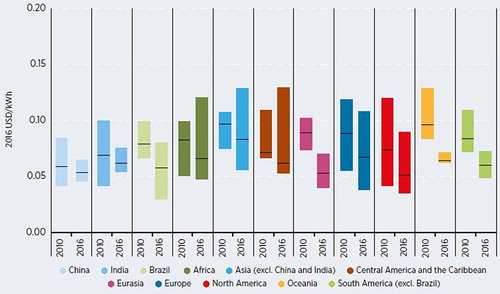
The development for onshore windfarms can be tracked for longer due to better data availability, which is why this paper uses onshore windfarms as case, and the global weighted average LCOE declined from USD 0.40/kWh in 1983 to USD 0.06/kWh in 2017, an 85% decline, but there are large variances depending on country and locations, see Figure 5. The results from this simple model is slightly lower – 0.05 USD/KWh. This is probably due to the fact that this model is presenting a relatively ideal case. In comparison, the global weighted average LCOE of offshore wind, which from 2010 to 2016 decreased from USD 0.17 to USD 0.14/kWh despite total installed costs increased by 8% during this period (IRENA 2018).

Figure 5. Regional weighted average LCOE and ranges of onshore wind, 2010–2016. Source: IRENA (2018).

Furthermore, it might be surprising to find that the LCOE for the opportunity cost, i.e. the dispatchable energy sources in Table 4, is higher than in Table 3. This is due to the effect that the four windfarms create less guaranteed output than 50% of the nominal/nameplate output. Hence, we need the effect of 2.18 opportunity energy sources to guarantee the output from the 1.72 windfarms that will always be producing energy. Vice versa, if the windfarm produced energy more than 50% of the time, then the opportunity LCOE would be lower than in Table 3. However, this is deterministic numbers.

To find out how uncertainty impacts we run a Monte Carlo simulation of the model. The results are shown in Figure 6. We see that the LCOE for the windfarm itself is as expected, with a mean of 58 USD/MWh, but the problem comes as soon as the output is going to be guaranteed. This gives a large opportunity LCOE, where the mean value is 93 USD/MWh, for the back-up dispatchable energy sources and hence and even larger Total LCOE of 151 USD/MWh, or almost three times the LCOE. This is under the ideal case of the windfarms having independent wind patterns. If the wind patterns are highly correlated, the result will be even worse.

Figure 6. LCOE for the four windfarms, the LCOE of the Opportunity (back-up, dispatchable energy sources) and the Total LCOE for all four windfarms.

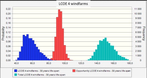
As we can see, this is substantially higher than many in the literature who report of doubling the LCOE when the integration costs are included. For example, Reichenberg et al. (2018) estimate that the LCOE for the entire system, which is similar to Total LCOE in this model, increases from roughly 40 EUR/MWh, or close to 50 USD/MWh, at zero market share to roughly 80 EUR/MWh, or close to 100 USD/MWh, at 99% market share. Many studies stop at 40% market share, such as Ueckerdt et al. (2013). They estimate a system LCOE of approximately 105 EUR/MWh, or roughly 130 USD/MWh.

This differences in result is due to some key factors of the modelling. First, they build a model and try to estimate the integration costs bottom-up. They assume that trade, or essentially a portfolio approach, will offset the non-dispatchable nature of wind. The simple model in this paper avoids the complexities of bottom-up and rather try to estimate how much back-up capacity is required to guarantee a certain nameplate output, and what the cost is. The weaknesses of this simple model are obvious compared to the more refined models of Reichenberg et al. (2018), Ueckerdt et al. (2013) – it is crude, simplistic and many costs are ignored or implicitly handled through the public information. The cost of trade is also ignored. This means that the opportunity cost is probably overstated in the short term, but as the crowding-out of dispatchable energy sources picks up, the opportunity costs will grow substantially and probably end up somewhere of what this model estimates.

However, this simple model has one indispensable advantage – it does not assume that a portfolio of windfarms can offset the fact that a windfarm produce energy less than half the time. Therefore, this simple model illustrates a crucial point that seems to be either ignored or forgotten in the debate surrounding windfarms – as soon as we promise a certain contribution to the grid, there is a large opportunity cost. This cost will increase through the duck curve over time.

There is one more advantage of the model presented here, it can be adjusted so that the life-span of the energy sources become the same. From Table 1 we see that 20 and 30 years are too short cost recovery periods/life-span. The fact is that if we extend the life-span to 60 years, for example, a windfarm will have to be reinvested twice. To illustrate the effect on the LCOE, we assume for simplicity that after 30 years the windfarm must be replaced by a new one. There is technological development over 30 years both in costs and performance, but since onshore windfarms are relatively mature technologies it is unlikely to be substantial. Indeed, after 2004 the installed cost of wind increased steadily with data for 2010 and 2011 suggesting a plateau in prices may have been reached (IRENA 2012).

The result is shown in Table 5, and we see that the LCOE for the windfarm increase as expected. The Total LCOE after 60 years is approximately as with the 30-year outlook in Table 4 – a result that does not alter itself by the introduction of uncertainty. This is because the relatively heavy discounting in the model (10%) and that the main driver for the LCOE is the installation costs and the PCF. This is exactly why the existing dispatchable power plants are so heavily penalised, as discussed earlier.

Table 5. Estimating the LCOE for four onshore windfarms using 60 years life-span.

Wind-farm	Nominal effect [MW]	Expected energy produced [MWh/year]	Installation costs [MUSD]	Depreciation [MUSD/year]	O&M costs [MUSD/year]	Total costs [MUSD/year]	LCOE [USD/MWh]	Opportunity LCOE [USD/MWh]	Total LCOE [USD/MWh]
1	350	1,318,380	517.0	17.2	9.5	26.7	49.7	79.1	128.7
2	350	1,318,380	517.0	17.2	9.5	26.7	49.7	79.1	128.7
3	350	1,318,380	517.0	17.2	9.5	26.7	49.7	79.1	128.7
4	350	1,318,380	517.0	17.2	9.5	26.7	49.7	79.1	128.7
Sum	1400	5,273,520	2,067.8	68.9	37.8	106.7	49.7	79.1	128.7

Windfarms can therefore best serve as additional source of energy to specific energy consumers, and not as a general contributor to the grid. Given that the literature significantly underestimates the opportunity costs, as argued above, the level of 40% market share as suggested by many in the literature seems to be much too high because of the volatility wind energy creates in the market.

This will have major long-term repercussions for the energy market due to the crowding-out. This evident from analysing the data for the period 2003–2015, as Burke and Abayasekara (2017) have done. They conclude that the long-run price elasticity of electricity demand in the US is around –1 for residences, between –0.3 and –0.6 for the commercial sector, –1.2 or larger for industry, and around –1 in total (10 percentage points increase results in a 10% drop in price). Their model is capable of explaining 98% of the variation in log electricity sales across US states, which is very good and it is mostly due to population development and average energy prices.

The population variable is a proxy for economic development since it has been known for decades that energy is one of the driving forces in socio-economic development (see Olsson 1994). Since the US EIA (2017) estimates that electricity use (sales plus direct use) will grow at an average of less than 1% per year to 2050, it is the average energy price in the market that will introduce most of the price impact. Thus, price volatility will not only introduce commercial risks for the customers, but it will render investments in dispatchable energy sources more uncertain than today as discussed earlier.

In turn, this will increase the LCOE for the dispatchable energy sources and hence the Opportunity LCOE for the windfarms as well. Naturally, this problem will grow as the market share of wind energy increases as many notes in the literature. In effect, the overall cost of the energy system will increase as the market share of non-dispatchable energy sources unless an economically viable way of storing the surplus energy they create is found.

In Section 4, a critical review of the research is provided, but next we must briefly discuss an interesting case in more details because it pinpoints and supports the issues discussed in this paper.

3.3. What can we learn from sustainable energy efforts in remote locations?

The El Hierro Island sustainable energy system case ‘embodies the first major Megawatt-level energy project by linking energy storage systems with wind power generation using water storage delivered by the pumping system between two artificial lakes' (Godina et al. 2015). In Frydrychowicz-Jastrzebska (2018), a thorough review is presented, along with many more cases, and the general finding is that

Studies have demonstrated that in the majority of locations, the achievement of the full energy self-sufficiency is an unrealistic purpose; the average annual percentage of renewable energy sources in the energy balance is estimated at the level between 30 and 80%.

The El Hierro Island case is no exception although significant improvements were made over the old energy system that relied solely on diesel generators, and the estimated share of renewable energy is up to 75% (Godina et al. 2015).

This occurs despite the advantageous topography of the island guarantees high wind levels of 7.24–8.42 m/s, and the La Caldera crater is a natural (upper) reservoir of the hydro-electric power plant located at 700 metres above sea level and can take 380,000 m³ of water.⁷ So, why did it happen? First, there were some obvious mismatch between the water reservoir’s capacity and the wind turbines’ energy production efficiency. This results in the necessity to limit the wind farm capacity to ensure grid stability and hence requires supplementation of energy from the diesel generator (Frydrychowicz-Jastrzebska 2018). Furthermore, the design criteria were that the hydroelectric system should be able to run for a maximum of 48 h when there was no wind. Overall the result was that the cost of electricity became high due to the complexity of the system. The electricity costs 3.5 times more than on continental Spain, and the VRE share of the total production in 2016 was 40.7%, in 2017, the best results were obtained in July, namely 79.4% and the average share in the first half of 2018 was 59.67% (Frydrychowicz-Jastrzebska 2018). This is very good results, but they came at a cost.

Since the island is small, any amounts of windmills will have similar wind conditions. The portfolio thinking will therefore not work, and the island is therefore reliant on a way to store the energy and for this purpose the hydro-electric, pump storage solution is innovative and good. This therefore boils down to risk and costs; the larger the water reservoirs, the more wind energy available to pump the water back, the better, but this comes at a cost. As shown in this paper, it is crucial to take into account the randomness of the wind and the uncertainty in the energy demand. This can be used to calculate the reservoir sizes. This was probably done, but due to constrained financial resources the reservoir was too little and the number of windmills was too little to fill up the upper reservoir fast enough.

Could 100% be achieved? Certainly, but the LCOE for the entire system would be very high, because the system had to handle natural variations with a safety buffer to avoid blackouts. For the pumping storage to be cost effective, it would therefore have to be large enough to fill an even larger reservoir. The windfarm would have to be dimensioned for even larger consumption. Unfortunately, a pumping storage can only work where the topography is beneficial such as in mountainous landscape so it would only work in special cases. In this case, the La Caldera crater has the necessary elevation above sea, but it is too small to handle the combination of the random variation in the weather and the demand.

If we translate this to a European level, the task would be even more daunting. Recall that only 13.6% of electricity in Europe is traded among countries (Batalla-Bejerano, Paniagua, and Trujillo-Baute 2019). As noted earlier, a solution like this would not only require enormous investments in transmission capacity, but also major changes in regulatory work in all the impacted countries.

The policy implications are clear. An energy system built solely on VRE, including hybrid systems where a pumped storage hydroelectric power plant serves as battery, will either be very expensive and/or run the risk of blackouts unless there are dispatchable energy sources. Due to the randomness of the wind, windfarms seem to be particularly problematic as source because the more randomness, the more buffering and the higher the costs. Solar energy would probably have worked better. However, also in such a setup, there are extra risks and -costs as the situation in California discussed earlier shows.

4. Discussion of research

This research was conducted using publicly available information, in particular US numbers from US EIA databases and the IRENA (2018) database. This introduces risks to the accuracy since various studies have various assumptions and are therefore not fully comparable, and public domain information is found to be unreliable (Ederer 2015). This is particularly true as the LCOE is the only common thread through the statistics and this approach has its weaknesses as discussed earlier. Along the same token, simplifications had to be made.

However, exactly because the numbers used in the example are from a large economy, and location-specific costs are ignored, the paper gives basis for conceptual discussions, which is the purpose. The modelling of the uncertainty, and simulation through Monte Carlo methods, reduce the aforementioned shortcomings since the uncertainty is larger than the loss of accuracy. Indeed, the introduction of Monte Carlo methods is an advantage in that a huge amount of model parameter variations (50,000) can be assessed.

The results are clear. Regardless of how we look at it, it will take at least four identical windfarms to guarantee the output of one under ideal/random weather conditions. Without providing any real statistics, the literature assumes that this can be solved by trade. With weather patterns being capable of impacting large geographical areas, and with increasing frequency as climate becomes more volatile – this seems an imprudent assumption. Furthermore, the assumption leads to a large underestimation of the true opportunity costs. The duck curve effects are essentially ignored – particularly its long-term effects.

The results also demonstrate the opportunity costs concerning windfarms and compared to the literature, it seems safe to suggest that the literature underestimates these costs significantly. Unfortunately, this simple model is incapable of dynamically modelling the log-term price impacts of increased market share of wind energy into the grid, as well as the trading- and grid costs themselves. Due to the large production variations of wind energy, this could have significant effects and obviously in negative direction.

This simple model did offer some limited insights into what a 60-year life-span would look like, and the importance of calculating the LCOE for the correct life-span for various technologies. When comparing the LCOE for different energy sources, it is crucial to compare the same life-span also because otherwise the investment perspective is skewed in favour of new technologies whereas the reality is probably the opposite as shown in Figure 1.

In the future, it would be desirable to study concrete examples of how grid-integration is achieved in specific locations with a major penetration of wind energy. This would allow more accurate modelling that provided here and hence also better policy support.

5. Closure and future work

While the research has clear shortcomings as discussed earlier, the overall picture of windfarms in terms of economics is clear. Windfarms can undoubtedly serve as additional source of in specific circumstances. However, there are significant opportunity costs that can change a decision completely – particularly as the market share of wind energy approaches a level where the volatility of the energy production significantly impacts the energy market through overproduction and lack of production. In turn, this will reduce the investments of dispatchable energy sources and create a more volatile energy system with cost spikes and increasing probability of blackouts.

Future work concerning the economics of windfarms should therefore revolve around properly calculating the Total LCOE for individual windfarms project under more realistic assumptions than done so far. Otherwise, we may end up investing into a technology that never had the potential of becoming a trustworthy source of energy except in special cases.

The policy implications are that an energy system consisting solely on VRE sources will either be very costly or run major risks of blackouts. Policy should therefore revolve around finding a good balance between VRE- and non-VRE sources where the variations of the different non-VRE sources and the energy demand itself must be taken into account properly.

Acknowledgements

I would like to thank the reviewers for constructive comments, and including directing my attention to the El Hierro Island case, which was unknown to me. The case not only shows the challenges of creating a completely sustainable energy system using renewables only, but it is small enough to understand.

Disclosure statement

No potential conflict of interest was reported by the author(s).

Notes

1 Some use Levelized Cost of Energy and others use Levelized Cost of Electricity.

2 Sometimes also referred to as ‘alternative cost’.

3 See U.S. Nuclear Regulatory Commission, Status of Subsequent License Renewal Applications, see www.nrc.gov/reactors/operating/licensing/renewal/subsequent-license-renewal.html.

4 Reported in https://www.cleanenergywire.org/news/renewables-hit-record-germany-h1-2019-outlook-uncertain.

5 Calculated based on data from https://www.eia.gov/electricity/data/eia860m/.

6 A good discounting factor is the Weighted Average Cost of Capital (WACC). In this simple case, we merely assume 10%, which is a relatively common discounting rate in real life. The WACC is often not far from 10%.

7 See Gorona del Viento at www.goronadelviento.es for details about the island (accessed on 20 November 2017).

References

- Aldersey-Williams, J., I. D. Broadbent, and P. A. Strachan. 2019. “Better Estimates of LCOE From Audited Accounts – A New Methodology with Examples From United Kingdom Offshore Wind and CCGT.” Energy Policy 128: 25–35. doi: 10.1016/j.enpol.2018.12.044
- Ball, J. 2018. “Why Carbon Price Isn’t Working: Good Idea in Theory, Failing in Practice.” Foreign Affairs 97 (4): 134–146.
- Batalla-Bejerano, J., J. Paniagua, and E. Trujillo-Baute. 2019. “Energy Market Integration and Electricity Trade.” Economics of Energy & Environmental Policy 8 (2): 53–67.
- Bazilian, M. D. 2015. “Power to the Poor: Provide Energy to Fight Powerty.” Foreign Affairs 94 (2): 133–138.
- Benes, K. J., and C. Augustin. 2016. “Beyond LCOE: A Simplified Framework for Assessing the Full Cost of Electricity.” The Electricity Journal 29: 48–54. doi: 10.1016/j.tej.2016.09.013
- Bruck, M., P. Sandhorn, and N. Goudarzi. 2018. “A Levelized Cost of Energy (LCOE) Model for Wind Farms That Include Power Purchase Agreements (PPAs).” Renewable Energy 122: 131–139. doi: 10.1016/j.renene.2017.12.100
- Burke, P. J., and A. Abayasekara. 2017. The Price Elasticity of Electricity Demand in the United States: A Three-Dimensional Analysis. Canberra: Centre for Applied Macroeconomic Analysis, The Australian National University. p. 34.
- CAISO. 2016. Fast Facts: What the Duck Curve Tells ut About Managing a Green Grid. Folsom, CA: California Independent System Operator (CAISO). p. 4.
- Doemeland, D., and J. Trevino. 2014. Which World Bank Reports are Widely Read? Policy Research Working Paper. Washington, DC: World Bank, Development Economics Vice Presidency, Operations and Strategy Unit, Group No. WPS6851. p. 32.
- Ebenhoch, R., D. Matha, S. Marathe, P. C. Munoz, and C. Molins. 2015. “Comparative Levelized Cost of Energy Analysis.” Energy Procedia 80: 108–122. doi: 10.1016/j.egypro.2015.11.413
- The Economist. 2014. “Curbing Climate Change.” The Economist. pp. 22–26.
- Ederer, N. 2015. “Evaluating Capital and Operating Cost Efficiency of Offshore Wind Farms: A DEA Approach.” Renewable and Sustainable Energy Reviews 42 (February): 1034–1046. doi: 10.1016/j.rser.2014.10.071
- Emblemsvåg, J. 2003. Life-Cycle Costing: Using Activity-Based Costing and Monte Carlo Methods to Manage Future Costs and Risks. Hoboken, NJ: John Wiley & Sons. p. 320.
- Emblemsvåg, J. 2016. Reengineering Capitalism: From Industrial Revolution Towards Sustainable Development. London: Springer. p. 332.
- Frydrychowicz-Jastrzebska, G. 2018. “El Hierro Renewable Energy Hybrid System: A Tough Compromise.” Energies 11. doi:10.3390/en11102812.
- Godina, R., E. M. G. Rodrigues, J. C. O. Matias, and J. P. S. Catalão. 2015. “Sustainable Energy System of El Hierro Island.” International Conference on Renewable Energies and Power Quality (ICREPQ’15), La Coruña.
- Hirst, E., and J. Hild. 2004. “The Value of Wind Energy as a Function of Wind Capacity.” The Electricity Journal 17 (6): 11–20. doi: 10.1016/j.tej.2004.04.010
- Ioannou, A., A. Angus, and F. Brennan. 2017. “Stochastic Prediction of Offshore Wind Farm LCOE Through an Integrated Cost Model.” Energy Procedia 107: 383–389. doi: 10.1016/j.egypro.2016.12.180
- Ioannou, A., A. Angus, and F. Brennan. 2018. “A Lifecycle Techno-Economic Model of Offshore Wind Energy for Different Entry and Exit Instances.” Applied Energy 221: 406–424. doi: 10.1016/j.apenergy.2018.03.143
- IRENA. 2012. Renewable Energy Technologies: Cost Analysis Series. Abu Dhabi: The International Renewable Energy Agency (IRENA), IRENA Innovation and Technology Centre. p. 56.
- IRENA. 2018. Renewable Power Generation Costs in 2017. Abu Dhabi: The International Renewable Energy Agency (IRENA), IRENA Innovation and Technology Centre. p. 158.
- Jägemann, C., M. Fürsch, S. Hagspiel, and S. Nagl. 2013. “Decarbonizing Europe’s Power Sector by 2050 – Analyzing the Economic Implications of Alternative Decarbonization Pathways.” Energy Economics 40 (November): 622–636. doi: 10.1016/j.eneco.2013.08.019
- Joskow, P. L. 2011. “Comparing the Costs of Internmittent and Dispatchable Electricity Generating Technologies.” American Economic Review 101 (3): 238–241. doi: 10.1257/aer.101.3.238
- Karagiannopoulos, L. 2018. “Norway Eyes Offshore Wind to Power Nyhamna Gas Processing Plant.” REUTERS, November 26.
- Loewen, J. 2019. “LCOE is an Undisclosed Metric That Distorts Comparative Analyses of Energy Costs.” The Electric Journal 32: 40–42. doi: 10.1016/j.tej.2019.05.019
- MAKE Consulting. 2017. Global Wind Turbine O&M. Arhus: MAKE Consulting.
- Mileva, A., J. Johnston, J. H. Nelson, and D. M. Kammen. 2016. “Power System Balancing for Deep Decarbonization of the Electricity Sector.” Applied Energy 162 (January): 1001–1009. doi: 10.1016/j.apenergy.2015.10.180
- Milligan, M., E. Ela, B.-M. Hodge, B. Kirby, D. Lew, C. Clark, J. De Cesaro, and K. Lynn. 2011. “Integration of Variable Generation, Cost-Causation, and Integration Costs.” The Electricity Journal 24 (9): 51–63. doi: 10.1016/j.tej.2011.10.011
- Myhr, A., C. Bjerkseter, A. Ågotnes, and T. A. Nygaard. 2014. “Levelised Cost of Energy for Offshore Floating Wind Turnbines in a Life Cycle Perspective.” Renewable Energy 66: 714–728. doi: 10.1016/j.renene.2014.01.017
- Nissen, U., and N. Harfst. 2019. “Shortcommings of the Traditional “Levelized Cost of Energy” [LCOE] for the Determination of Grid Parity.” Energy 171: 1009–1016. doi: 10.1016/j.energy.2019.01.093
- Olsson, L. E. 1994. “Energy-Meteorology: A New Discipline.” Renewable Energy 5: 1243–1246. doi: 10.1016/0960-1481(94)90157-0
- Reichenberg, L., F. Hedemus, M. Odenberger, and F. Johnsson. 2018. “The Marginal System LCOE of Variable Renewables – Evaluating High Penetration Levels of Sind and Solar in Europe.” Energy 152: 914–924. doi: 10.1016/j.energy.2018.02.061
- Smart, G., A. Smith, E. Warner, I. B. Sperstad, B. Prinsen, and R. Lacal-Arántegui. 2016. IEA Wind Task 26 – Offshore Wind Farm Baseline Documentation. Golden, CO: National Renewable Energy Laboratory, U.S. Department of Energy Office of Energy Efficiency & Renewable Energy. p. 30.
- Stacy, T. F., and G. S. Taylor. 2019. The Levelized Cost of Electricity From Existing Generation Resources. Washington, DC: Institute for Energy Research (IER). p. 34.
- Stehly, T., D. Heimiller, and G. Scott. 2017. 2016 Cost of Wind Energy Review. Golden, CO: National Renewable Energy Laboratory, U.S. Department of Energy Office of Energy Efficiency & Renewable Energy. p. 38.
- Tran, T. T. D., and A. D. Smith. 2017. “Evaluation of Renewable Energy Technologies and Their Potential for Technical Integration and Cost-Effective use Within the U.S. Energy Sector.” Renewable and Sustainable Energy Reviews 80 (April): 1372–1388. doi: 10.1016/j.rser.2017.05.228
- Tran, T. T. D., and A. D. Smith. 2018. “Incorporating Performance-Based Global Sensitivity and Uncertainty Analysis into LCOE Calculations for Emerging Renewable Energy Technologies.” Applied Energy 216: 157–171. doi: 10.1016/j.apenergy.2018.02.024
- Ueckerdt, F., L. Hirth, G. Luderer, and O. Edenhofer. 2013. “System LCOE: What are the Costs of Variable Renewables?” Energy 63: 61–75. doi: 10.1016/j.energy.2013.10.072
- USDE. 2015. Wind Vision: A New Era for Wind Power in the United States. Springfield, VA: United States Department of Energy, Wind and Water Power Technologies Office.
- US EIA. 2017. Annual Energy Outlook 2017 with Projections to 2050. Washington, DC: US Energy Information Administration. pp. 64.
- US EIA. 2019. Levelized Cost and Levelized Avoided Cost of New Generation Resources in the Annual Energy Outlook 2019. Washington, DC: US Energy Information Administration. pp. 25.