Assessment of wave power stability and classification with two global datasets

ABSTRACT

Global distribution of the wave climate and energy using a re-analysis dataset provides the opportunity to study spatio-temporal variation of different parameters, and offers inputs for future sustainability plans. The study assesses two global scale products ERA5 and ERA-Interim, evaluating differentiation in wave climate and energy parameters. Results compare the performance globally and analyse the rate of change for wave power and its persistence characteristics. Based on results for the spatial distribution and rate of change for wave characteristics, wave power and joint distributions are expected to increase. The study provides novel information with a wave energy development index and rate of change globally, suggesting the most appropriate areas for further assessment based on the discussed criteria.

KEYWORDS:

• Wave energy
• metocean condition
• climate persistence
• ERA-interim
• ERA5

1. Introduction

In 2018, the Intergovernmental Panel of Climate Change (IPCC) published its report concerning the contribution of anthropogenic emissions and the differentiation of climate patterns (IPCC 2018). To mitigate the hazardous effects associated with Climate Change, several actions have been proposed with most prominent the decarbonisation of energy systems and transition into energy systems with higher renewable sources (United Nations 2015). However, in order to achieve the ambitious targets of decarbonisation and obtain long-term sustainability, all indigenous resources have to be utilised.

Jacobson et al. (2017) assessed the feasibility of a 100% carbon-free energy system powered by available renewable resources. The work underlined the necessity of offshore energies and the integral part they have to play for the energy transition. Spearheading the change is offshore wind; however, the study indicated that higher expected development for offshore wind will not be realised without multi-renewable generation. Therefore, it was also suggested that ocean energies are also expected to play a significant role, with wave energy having the largest share in installed nameplate capacity globally, with expected 307 GW by 2050.

Among offshore renewable energies, wave energy has the highest energy density waves that can be highly predictable (Zheng, Wang, and Li 2017) and has several positive environmental benefits (Soukissian et al. 2017). Leeney et al. (2014) gave a thorough description of marine energy development based on existing activities, it recorded numerous potential ‘spill-over’ benefits, such as lower visual impacts, development of local ecosystems, for example, artificial reef generation by marine energy converters infrastructure. Moreover, local communities do not oppose the development of marine renewable energy, since they do not find them as intrusive (Alexander, Wilding, and Jacomina Heymans 2013). Voke et al. (2013) assessed the value of the marine environment at the United Kingdom and found that the visual impact of marine renewables was enhanced due to their reduced visual impacts. In addition, it was concluded by the interviews of visitors and population that the economic activities at the area were not endangered (i.e. such as tourism), hence reducing the social impacts such as Not In My Back Yard (NIMBY). However, the wave resource is expected to experience changes, what may have a domino effect on many industries, and management of disasters such as storms and flooding (IPCC 2018).

Without the use of multi-renewable generation, energy systems are more vulnerable to Climate Change and weather variations, with expected production affected (Ravestein et al. 2018) requiring massive back-up capacity and affecting energy costs (Schlachtberger et al. 2018). However, temporal production benefits by multi-generation have been identified, and combination of offshore wind and wave farms can actively reduce the variable energy production (Soukissian et al. 2017; Lavidas and Venugopal 2018c; Astariz and Iglesias 2016).

Extracting power from waves requires a multi-dimensional approach, is highly dependent on the available resource and is sensitive to change (Mackay, Bahaj, and Challenor 2010). Waves are dependent on three major characteristics (i) significant wave height ($H_{m0}$), (ii) energy period ($T_e$), (iii) wave direction. Another layer of complexity is the different operating principles of Wave Energy Converters (WECs) and their depth applicability considerations. Currently, there are $\ge 50$ devices (Rusu and Onea 2018). There is no “silver” bullet or universal solution for WECs as they depend on depth and resource characteristics (Babarit et al. 2012). All use a power matrix, the equivalent to a power curve, to estimate the production of carbon-free electricity per seastate. However, the selection of a WEC is far from a trivial process, and there is the need to properly assess the long-term wave resource changes that directly will affect energy production (Fairley et al. 2020). Wave resource potential and hence potential power production can vary even at sites with close geographic proximity, therefore multiple marine energy sites can reduced times of non-generation (Fairley et al. 2017).

Introducing wave energy into electricity systems can result in reducing needs for back-up generation and energy storage, leading to large reductions in electricity costs and emissions, of up to 40 and 60%, respectively (Friedrich and Lavidas 2017). Underlying the need to properly select the wave energy converter in line with other studies (Luppa et al. 2015; Guillou and Chapalain 2018; Lavidas and Venugopal 2018b), as the benefit seems to be diminished for Levelized Cost of Energy (LCOE) of ≥0.35 £/kWh. Guillou and Chapalain (2018) examined that between seasons and months, the variations on potential energy output can vary ≈50%, and the selection of a wave energy converter should be considered in depth as well as its performance over long-term seasonal patters.

With increases at available computational power, assessment and in particular wave energy resource quantifications have been increasing ; however, differences in wave energy resource estimations still can exist (Reguero, Losada, and Méndez 2015) not only because of different models (Lavidas and Venugopal 2018a) but also due to estimation methodologies with, resulting in varied energy estimates for resources ≈32,000 TWh/year (Mørk et al. 2010), 18,500 TWh/year (Gunn and Stock-Williams 2012), and recently ≈16,025 TWh/year (Reguero, Losada, and Méndez 2015).

This study aims to examine two resource characteristics in global scale that is the most prevalent in WECs power production, the $H_{m0}$ and $T_e$. Focus is given on these two parameters, as they are most vital for resource estimation and indicates the expected power production. Through, directionality is also highly important, such information is not often disclosed in power matrices. In addition, due to the coarseness of the global dataset, directionality changes for wave energy application will be more useful with downscaled spatial high-resolution modelling that also captures better local bathymetric and topographic effects.

Our analysis uses the prism of climate persistence to assess the quantitative statistical metocean characteristics, which allow us to assess the long-term rate of change that is expected to affect power production. Two global re-analysis datasets are used to estimate the statistics and wave resource characteristics. These can be vital for proper selection of WECs, which benefit immensely by knowing the areas where metocean conditions will see the minimum changes and potentially match their power matrix better.

The analysis compares metocean hindcast conditions, examining differences and similarities for statistical metocean attributes, quantifying and comparing the wave energy resource. Furthermore, a Wave Energy Development Index (WEDI) is used to note regions that may prove interesting for wave energy farms, by considering the relationship between maximum resource and average conditions. Finally, the rate of change is estimated, indicating regional differences, and discussing the distribution of metocean conditions necessary for power production. Incorporating the rate of change allows us to classify wave power regions that have good potential while having higher stability, subsequently, these can benefit from future and more detailed high-resolution spatio-temporal studies.

2. Materials and methods

Two datasets are analysed the ERA5 (Hersbach et al. 2019) and ERA-Interim (Dee et al. 2011), both provided by European Centre for Medium-Range Weather Forecasts (ECMWF) (ECMWF 2020). The datasets are based on in-house methods by ECMWF (Hersbach et al. 2019), common premise is the use of the same wave model to produce the wave data (WAM) which are then re-analysed, minimising result discrepancies. However, there are differences between the two datasets, predominately in the spatial and temporal resolutions.

In spatial terms, there is a significant magnitude reduction in spatial resolution, from $\approx {0.7}^{\circ }$ at ERA-Interim to ${0.36}^{\circ }$ in ERA5. Although the hindcast products are available in several resolutions, we used a similar range of ${0.5}^{\circ }$ over longitude and latitude for both datasets through the Meteorological Archival and Retrieval System (MARS). The time output frequency for ERA5 is 1-h, while for ERA-Interim is 6 h. Finally, ER5 uses a different Integrated Forecasting System (IFS), and slowly (after 2020) ERA5 will replace ERA-Interim (Hersbach et al. 2019).

Climate analysis for any type of renewable resource requires a minimum duration of 10 years (World Bank 2010; Ingram et al. 2011; Smith and Maisondieu 2014; Lavidas, Venugopal, and Friedrich 2017). However, to obtain a good understanding of climate conditions and their persistence Climatological Standard Normals (CSN) are necessary, with a suggested duration ≥30 years (World Meteorological Organization 2017). This analysis includes 30 years of data from 1989 to 2018, therefore ensuring that this first layer classification adheres to international standards.

Key metocean parameters from respective databases are used to assess climate statistics as mean values, wave energy, 99th percentile and Rate of Change (RC). Subsequently, the slope of the main variables is used to discuss the effects on wave energy and expected variations. Wave energy is expressed as energy density contained per unit crest of a wave, with units in W/m or kW/m. Starting from a simplistic approach wave energy flux estimations considers depth as having little or no effects, with wave energy the summation of kinetic ($E_{\mathrm{k}\mathrm{i}\mathrm{n}}$) and potential energy ($E_{\mathrm{p}\mathrm{o}\mathrm{t}}$) per unit surface area of a wave.(1) $E_{\mathrm{w}\mathrm{a}\mathrm{v}\mathrm{e}}=E_{\mathrm{k}\mathrm{i}\mathrm{n}}+E_{\mathrm{p}\mathrm{o}\mathrm{t}}=\frac{1}{8}\cdot \rho \cdot g\cdot H^2\cdot C_g$(1) (2) $C_g=\frac{1}{2}\cdot [1+\frac{2k\cdot h}{\sinh (2k\cdot h)}]\cdot \frac{T\cdot \sqrt{\frac{g}{k}\cdot \tanh (k\cdot h)}}{T}$(2) ρ water density, g gravitational acceleration, $H=2\alpha$ wave height (α = amplitude), T wave period. Potential energy per unit of wave crest (height) depends on the wave group and its celerity (see Equations (1(1) $E_{\mathrm{w}\mathrm{a}\mathrm{v}\mathrm{e}}=E_{\mathrm{k}\mathrm{i}\mathrm{n}}+E_{\mathrm{p}\mathrm{o}\mathrm{t}}=\frac{1}{8}\cdot \rho \cdot g\cdot H^2\cdot C_g$(1) ) and (2(2) $C_g=\frac{1}{2}\cdot [1+\frac{2k\cdot h}{\sinh (2k\cdot h)}]\cdot \frac{T\cdot \sqrt{\frac{g}{k}\cdot \tanh (k\cdot h)}}{T}$(2) )). The relation between wave crest length (${\lambda }_{\mathrm{w}\mathrm{a}\mathrm{v}\mathrm{e}}$ ), depth (h) and period are based on the dispersion relationship. Waves are a summation of different wave numbers and frequencies interacting in the area, depending on the energy density travelling with varied frequency (f) and directions (θ), expressed by the $2D$ spectrum over $E(f,\theta )$. For wave energy, the preferred representative wave height notation is the significant wave height ($H_{m0}$) (see Equation (3(3) $H_{m0}=4\cdot \sqrt{m_o}$(3) )), and the preferred period is the energy period $T_e$ (see (4(4) $T_e=\frac{m_{-1}}{m_n}$(4) )), derived from the zeroth and first moments of the spectrum, see (5(5) $m_n={\int }_0^{2\pi }{\int }_0^{\mathrm{\infty }}{f}^{n}E(f,\theta )\mathrm{d}f\cdot \mathrm{d}\theta$(5) ).(3) $H_{m0}=4\cdot \sqrt{m_o}$(3) (4) $T_e=\frac{m_{-1}}{m_n}$(4) (5) $m_n={\int }_0^{2\pi }{\int }_0^{\mathrm{\infty }}{f}^{n}E(f,\theta )\mathrm{d}f\cdot \mathrm{d}\theta$(5) $T_e$ is a quantity that is connected with the measured period, specifically, it is assumed that $T_e=1.14T_z$, and $T_e={\alpha }_{\mathrm{w}\mathrm{a}\mathrm{v}\mathrm{e}}\cdot T_{\mathrm{p}\mathrm{e}\mathrm{a}\mathrm{k}}$, with ${\alpha }_{\mathrm{w}\mathrm{a}\mathrm{v}\mathrm{e}}$ dependent on the wave spectrum and with values close to unity. Finally, the $H_{m0}$ that is introduced to the calculation, includes the overall wave height of combined seas from wind-generated and swell waves. Therefore, considering that waves are not linear, and their energy content is affected by the spectral moments for $H_{m0}$ and $T_e$, the wave energy flux of per width metre crest (kW/m) is expressed by Equation (6(6) $P_{\mathrm{w}\mathrm{a}\mathrm{v}\mathrm{e}}=\frac{\rho \cdot g^2\cdot H_{m0}^2\cdot T_e}{64\cdot \pi }$(6) ).(6) $P_{\mathrm{w}\mathrm{a}\mathrm{v}\mathrm{e}}=\frac{\rho \cdot g^2\cdot H_{m0}^2\cdot T_e}{64\cdot \pi }$(6) However, the energy content itself requires more information in order to make useful decisions, the Wave Energy Development Index (WEDI) expresses the ratio of annual average wave power ($P_{\mathrm{w}\mathrm{a}\mathrm{v}\mathrm{e}}$) to the maximum storm wave power ($J_{\mathrm{w}\mathrm{a}\mathrm{v}\mathrm{e}}$) that every offshore device or structure will have to absorb, WEDI measures the severity and penalises areas with a high extreme/storm conditions, see Equation (7(7) $\mathrm{W}\mathrm{E}\mathrm{D}\mathrm{I}=\frac{\overline{P_{\mathrm{w}\mathrm{a}\mathrm{v}\mathrm{e}}}}{J_{\mathrm{w}\mathrm{a}\mathrm{v}\mathrm{e}}}$(7) ) (Hagerman 2001; Akpinar et al. 2012; Lavidas, Venugopal, and Friedrich 2017).(7) $\mathrm{W}\mathrm{E}\mathrm{D}\mathrm{I}=\frac{\overline{P_{\mathrm{w}\mathrm{a}\mathrm{v}\mathrm{e}}}}{J_{\mathrm{w}\mathrm{a}\mathrm{v}\mathrm{e}}}$(7) The Rate of Change (RC), takes into account the statistical parameters of wave energy (e.g. mean wave energy ($\mathrm{\Delta }{P}_{\mathrm{w}\mathrm{a}\mathrm{v}\mathrm{e}}$ )), and estimate the resource persistence over their time difference ($\mathrm{\Delta }T$) (see Equation (8(8) $\mathrm{R}\mathrm{C}=\frac{\mathrm{\Delta }{P}_{\mathrm{w}\mathrm{a}\mathrm{v}\mathrm{e}}}{\mathrm{\Delta }T}$(8) )).(8) $\mathrm{R}\mathrm{C}=\frac{\mathrm{\Delta }{P}_{\mathrm{w}\mathrm{a}\mathrm{v}\mathrm{e}}}{\mathrm{\Delta }T}$(8)

3. Results

3.1. Metocean conditions

Global mean value of $H_{m0}$ based on ERA5, ERA-Interim have similar spatial distribution, with the highest waves encountered near Southern latitudes (30–${60}^{\circ }$ S), off the coast of Antarctica with 4.5–5 m, and at Northern latitudes (40–${60}^{\circ }$ N) at the Atlantic and Pacific Oceans (see Figure 1). Both exhibit similar evolution with ERA5 having slightly higher values near Antarctica. ERA-Interim exhibits increased $H_{m0}$ at North Atlantic with mean values closer to the 4.5 m.

Figure 1. Mean $H_{m0}$ in m based on (a) ERA5, (b) ERA-Interim and their (c) difference (between ERA5 and ERA-Interim).

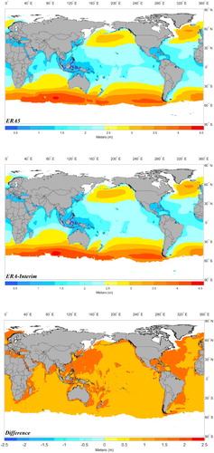
The 99^th percentile indicates that majority of the time both at higher Northern and lower Southern latitudes $H_{m0}$ is $\le 9$ m (see Figure 2). Both datasets have a similar spatial distribution for harsh events; however, ERA-Interim illustrates higher values when compared to ERA-5. The percentile value reveals that severe events occur with similar magnitudes near the Poles. At Equatorial regions (${30}^{\circ }$ S–${30}^{\circ }$ N), mean values drop to $\le 4$ m, while at Oceans centres and near continental coastlines magnitudes are reduced to 3 m. Lower values are found in the Mediterranean, North Australia, the complex of islands New Guinea, Indonesia and the Philippines with $\le 4$ m, although the 99^th of $H_{m0}$ is $\le 6$ m indicating harsh events can occur often.

Figure 2. 99th percentile of $H_{m0}$ in m based on (a) ERA5, (b) ERA-Interim and their (c) difference (between ERA5 and ERA-Interim).

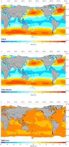
For $T_e$, the spatial distribution is more evenly spread, at lower latitudes (30–${60}^{\circ }$ S), low frequency (high periods) have a magnitude $\ge 9$  sec, indicating that the regions are swell dominated (Figure 3). ERA5 experiences a decrease by $\approx 1$ sec at central parts of the Pacific Ocean, near the Southern Ocean and Pole there is a consistent difference of 1 sec when compared with ERA-Interim. Closer at the coasts of Australia, New Guinea and up to Japan, mean $T_e$ values are $\approx$7–8 sec, while off the coast of both North and South America period value are ≥9–10 sec, indicating that higher swell waves reach the coasts of Americas with primary origin Western coasts of the Pacific ocean. Similar behaviour is encountered at the Atlantic Ocean, where higher frequency waves occur off Eastern American coastlines, travelling towards the European and African coastlines, amplifying their $H_{m0}$ and increasing their wave period (lower frequencies).

Figure 3. Mean $T_e$ in s (m) based on (a) ERA5, (b) ERA-Interim and their (c) difference (between ERA5 and ERA-Interim).

The Indian Ocean has similar values of $T_e$ and $H_{m0}$, as the ones at Eastern Japan, Australia, New Guinea, and Northern parts of the Arabian Sea with magnitudes from 6–7.5  sec, indicating low swell seas. When comparing mean values, it is evident that ERA-Interim is lower by ≈1 sec along most coastal regions (near the coasts), when ERA5 is considered as a baseline. Majority of the domain has a very good agreement, and both datasets present similar values at deep waters. Greater differences are found in areas with complex coastlines, such as the Gulf of California, where wave periods at coastal inlets have a higher alterations with ERA5 hindcasting ≈5 sec less. Similar differences are also present at the Indonesia, Jakarta and Singapore regions, indicating that closer to coastlines, there are increased differences (see Figure 3).

In the Mediterranean, 99^th percentile indicates that most sea states are $T_e\le 10$  sec, describing smaller swells that originate from the Western side of the Basin. Central parts of the Pacific, coastal Atlantic European and African regions experience higher swells, as indicated by $T_e$ description being usually ≤14 sec and with a mean value above 10  sec. However, the ERA-Interim shows consistent higher percentiles values in open Seas and lower in enclosed Basins (i.e. Mediterranean and Black Sea), see Figure 4.

Figure 4. 99^th percentile of $T_e$ in s (m) based on (a) ERA5, (b) ERA-Interim and their (c) difference (between ERA5 and ERA-Interim).

Regions at deeper ocean waters have very similar magnitudes; however, across both datasets, there is a difference of 0.5 m, ERA-Interim has lower magnitudes and differences consistently higher at nearshore coastal areas. Specifically, in the Mediterranean, regardless of depth, ERA-Interim waves are consistently lower than ERA5. The only region that a higher difference occurs is off the coast of Antarctica (see Figure 1). The difference in magnitudes is amplified when higher waves are examined, the 99^th percentiles value present a significant deviation between datasets. At very deep Ocean depths, highest waves have little differences; near the coastlines, ERA5 is ≈0.51 m lower when compared to ERA-Interim.

3.2. Wave energy

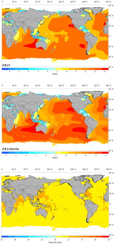
As the wave energy flux is dependent predominately on the square of $H_{m0}$ (see Figure 6(6) $P_{\mathrm{w}\mathrm{a}\mathrm{v}\mathrm{e}}=\frac{\rho \cdot g^2\cdot H_{m0}^2\cdot T_e}{64\cdot \pi }$(6) ), it should be expected that regions with larger $H_{m0}$ magnitudes encompass higher density. In terms of $P_{\mathrm{w}\mathrm{a}\mathrm{v}\mathrm{e}}$, both datasets are similar at the Antarctic Ocean between longitudes of ${50}^{\circ }$–${120}^{\circ }$ East, with fluxes from 105 to 120 kW/m. Mid-latitudes, at the Pacific, Indian and Atlantic ocean are characterised with ≈40 kW/m (see Figure 5). At higher latitudes (30–${60}^{\circ }$ S), the content almost doubles in magnitude with ≥65 kW/m, especially at Scotland which is exposed to some of the harshest environments in the Northern Hemisphere.

Figure 5. Spatial distribution of mean $P_{\mathrm{w}\mathrm{a}\mathrm{v}\mathrm{e}}$ in kW/m based on (a) ERA5 (b) ERA-Interim.

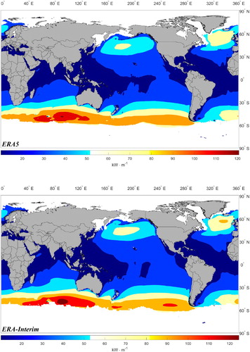
ERA-Interim has higher values of spectral characteristics ($H_{m0}$, $T_e$) presents higher $P_{\mathrm{w}\mathrm{a}\mathrm{v}\mathrm{e}}$ for extended spatial regions (see Figure 5). ERA-Interim has a larger area coverage with $P_{wave}\ge 90$ kW/m. At enclosed Basins such as the Mediterranean, $H_{m0}$ value has lower magnitude differences, while wave period is increased, although this does not lead to high deviations between wave energy content, with magnitudes ≤20 kW/m, though ERA-Interim still is higher than ERA5 by ≈10–15%.

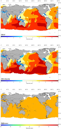
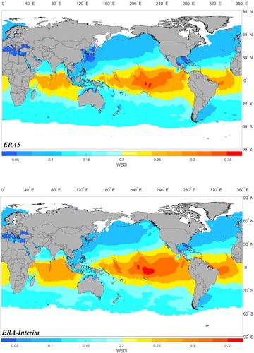
The WEDI ratio can be helpful in the determination of energetic areas that also experience ‘less’ harsh events. Ideally, a region will have a high mean value and low maximum, showcasing the potential of high energy content without compromising survivability. ERA-Interim over-estimates $H_{m0}$ at nearshore areas, and it is evident that WEDI values penalise this dataset more often at the nearshore (see Figure 6). As the wave climate in the mid-latitudes is dominated by ‘smaller’ swells, WEDI shows greater values there which mean higher stability of wave energy in connection to their extreme values. WEDI reaches its lowest at high latitudes in the Northern hemisphere, as higher swells and storm conditions can prove catastrophic.

Figure 6. Spatial distribution of WEDI (a) ERA5 (b) ERA-Interim.

3.3. Rates of change

While metocean conditions and power content are vital to assess and categorise a region/site, the rate of change (RC, see Figure 8(8) $\mathrm{R}\mathrm{C}=\frac{\mathrm{\Delta }{P}_{\mathrm{w}\mathrm{a}\mathrm{v}\mathrm{e}}}{\mathrm{\Delta }T}$(8) ) can indicate the ‘stability’ of the resource temporally. With the use of long-term data, it reveals the stability and resource alterations. A positive trend indicates that the $P_{\mathrm{w}\mathrm{a}\mathrm{v}\mathrm{e}}$ is increasing with a specific rate, while a negative value indicates that it is decreasing. Based on the hincast data duration, the regions that have a good resource with lower RC can be identified on a preliminary scale, and be the work of further downscaled studies. Allowing us to identify regions which are stable enough support wave energy converters without the re-tuning for optimised operation.

At the Northern Hemisphere RC indicates a mixture of changes in magnitude. At the Northern Pacific (40–60${}^{\circ }$ N) RC is nearly zero, in the central part of the region; however, there is a clear reducing trend by 200–300 W/m/year at the central region of the Northern Pacific, see Figure 7. Relative reductions are recorded at Northern coasts of Scotland, the Norwegian and Barents Sea by ≈100 W/m/year. Close to the East coastlines of North America at the Atlantic, RC shows a highly positive increase by ≥200 W/m/year. Both datasets have the same magnitudes with ERA-Interim indicating a larger spatial distribution at the Northern Hemisphere. At the Southern Hemisphere, ERA5 indicates a larger spatial distribution of the RC (see Figure 8(8) $\mathrm{R}\mathrm{C}=\frac{\mathrm{\Delta }{P}_{\mathrm{w}\mathrm{a}\mathrm{v}\mathrm{e}}}{\mathrm{\Delta }T}$(8) ).

Figure 7. Rate of Change (RC) for mean $P_{\mathrm{w}\mathrm{a}\mathrm{v}\mathrm{e}}$ in kW/m/yr (a) ERA5 (b) ERA-Interim (c) difference (between ERA5 and ERA-Interim).

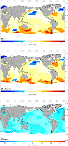
Equatorial areas, located at $\pm {20}^{\circ }$ from the Equator, have similar magnitudes of RC with a positive trend at both dataset of ≈100–150 W/m/year. This similarity is also expressed at both datasets, for the Mediterranean and Black Sea. In the Southern Hemisphere on the other hand, the trends indicate that majority of locations from (30–${60}^{\circ }$ S) have a high positive $\mathrm{R}\mathrm{C}\ge 150$ W/m/year. The region that saw the highest increase in wave power resource per annum, is Chile, followed by Southern coast of Australia, and South-western regions of the African continent. Therefore, a global classification should not only consider the energy content of sea states, but also the RC which may occur and affect the distributions. Ideally, the classification should consider the most energetic seas with the minimum or no rate of change. The reason for that is to ensure that wave power converters will not need re-adjustments in their characteristics and will deployed with higher confidence over the long-term.

4. Discussion

In order to obtain a reliable assessment of the global wave resources, it is important to use validated datasets and be aware of their limitation and differences (Lavidas and Venugopal 2018a). With a wide array of datasets, available reproduction of the wave climate/energy content can differ in its spatial distribution based on the model used and configuration. This was highlighted by the work of Fairley et al. (2020), which used a k-clustering method to distinguish between wave energy regions. Their analysis classified the global regions according to power content and determined that 55% of most areas are exposed to moderate resources.

This study expands and furthers with a global assessment of the wave power resource to include long-term stability and a wave energy development index considering the changing climate. With a starting point the year 1989 RC examined the regions for which the variables have changed in a positive or negative manner. While this was not an extensive Climate Change analysis, it recorded the trend for which the $P_{\mathrm{w}\mathrm{a}\mathrm{v}\mathrm{e}}$ changes, predominately indicating increasing trends in the southern hemisphere and some decreasing trends in the northern hemisphere. Regions located at mid-latitudes experience little changes. This can be beneficial as it can emphasise higher stability over time. Therefore, areas with such characteristics can be considered further for sustainable development, through the deployment of wave energy farms, as they indicate a low rate of change and moderate persistent resource.

This is a preliminary analysis to identify regions that have the ‘right’ mixture of wave power, WEDI and show no major changes and can be further investigated by nested models of higher resolution to characterise the nearshore regions. Regions that can benefit are the Mediterranean, India and the South East complex of island Nations between the East Indian Ocean and South China Sea. However, it is important to keep in mind the differences between basic wave quantities across the datasets, as they are often used as boundary conditions for higher fidelity models. The ERA5 due to its temporal resolution has overall higher mean values at deeper locations, though with reduced spatial scale. The ERA-Interim product has similar hindcast of high waves but they tend to cover spatially a larger area, leading to over-estimations of extremes even as boundary conditions.

5. Conclusions

To ensure proper analysis of long-term variability, 30 years of data were analysed, results indicated that both datasets reproduce similar spatial distributions patterns. However, it can be a general notice that ERA5 has higher values over ERA-Interim. For $H_{m0}$, higher differences are encountered in the Mediterranean, North Atlantic regions with ERA5 having ≈0.5 m increased estimates. Nearshore region throughout the globe showcase a positive difference of the same magnitude for ERA5; however, it has to be kept in mind that such databases are not suitable for nearshore assessments.

In contrast, both datasets have near-zero differences at the Poles where highest waves, both in mean and percentile values were found. Differences between energy period are less than that of $H_{m0}$, with both datasets having very close distribution in magnitudes. The findings display similarity with Reguero et al. (2012), with spatial distribution being more in-line with ERA-Interim. Our results also support the proposal by Fairley et al. (2020) to focus more on specific class regions for wave energy development that are most commonly found. Moderate resources have lower variability, enhanced stability and can be accessed by a large number of countries.

Asides the mean values and differences of spatial distribution for the parameters, we also examined the 99th percentile. Analysis by ERA-Interim shows a large difference with higher extreme events in high latitudes at deeper locations when compared to ERA5. WEDI indicates the suitability of wave energy extraction in an area; the analysis indicates that the mid-latitudes experience a higher ratio of mean wave power to extreme values, indicating the suitability for development.

ERA-Interim has slightly higher magnitudes at Poles of wave energy following the 99th percentile trend. At the Pacific Ocean, most energetic areas are the lower South Americas ≈90 kW/m, Western Australia ≈85 kW/m, the North-East of US coastline and Canada ≈50–80 kW/m. At the Atlantic, most energetic areas are Ireland, United Kingdom ≈70–80 kW/m, and the Western Spanish coasts ≈50 kW/m. At the Southern Hemisphere, South Africa has the highest fluxes ≈50–70 kW/m. Throughout the Mediterranean wave energy has similar magnitudes ≈10–15 kW/m.

Higher conditions are met in the enclosed waters between the coastlines of Indonesia, Philippines and Malaysia ≈20–30 kW/m, as the majority of Easterly incoming swells are transformed and dissipated, analogous conditions are recorded for the Indian coastlines. Both datasets have greater similarity in deep mid-latitude regions, majority of differences are located nearshore and at the Poles. Rate of change for wave power is predominately positive, with reductions in the Norwegian Sea and North Pacific. Wave periods have little change over the datasets analysis, with $P_{\mathrm{w}\mathrm{a}\mathrm{v}\mathrm{e}}$ being mostly influenced by the changes in $H_{m0}$. This is also pointed out by Reguero, Losada, and Mendez (2019), our analysis shows similar trends in the same spatial domain.

With regard to wave energy potential areas, the power content is not enough to be used as an indicator, the balance between mean high energy flux and the potential catastrophic effects by harsh events was evaluated by the WEDI index. For both datasets, the WEDI distribution is similar only having slightly higher values in the Mediterranean and Equatorial regions, indicating that ERA-Interim over-estimates when compared with ERA5. The RC expresses that it should be expected that wave power will be increased, altering the joint distributions. Selecting a site for WEC farm should always consider not only the energy levels but also the hazardous conditions that can be disastrous for the array, so moderate resources seem to be favourable.

Geolocation information

The analysis is global with latitude ${180}^{\circ }$ to $-{180}^{\circ }$ and longitude $0^{\circ }$ to ${360}^{\circ }$.

Acknowledgments

The authors would like to thank the reviewers for their constructive comments, which helped in the improvement of the manuscript. The second author (BK) was supported by the Hakubi Center for Advanced Research at Kyoto University, and JSPS Grants-in-Aid for Scientific Research – KAKENHI – supported by the Ministry of Education, Culture, Sports, Science, and Technology-Japan (MEXT). Both authors have been supported by International Integrated Wave Energy Research Group (IIWER, www.iiwer.org), that fosters and encourages collaboration of interdisciplinary research in wave energy as a non-profit organisation.

Disclosure statement

No potential conflict of interest was reported by the authors.

Additional information

Funding

The second author (BK) was supported by the Hakubi Center for Advanced Research at Kyoto University, and JSPS Grants-in-Aid for Scientific Research –KAKENHI- supported by the Ministry of Education, Culture, Sports, Science, and Technology-Japan (MEXT). Both authors have been supported by International Integrated Wave Energy Research Group (IIWER, www.iiwer.org), that fosters and encourages collaboration of interdisciplinary research in wave energy as a non-profit organisation.

References

- Akpinar, A., G. P. van Vledder, M. H. Kömürcü, and M. Özger. 2012. “Evaluation of the Numerical Wave Model (SWAN) for Wave Simulation in the Black Sea.” Continental Shelf Research 50–51: 80–99. http://linkinghub.elsevier.com/retrieve/pii/S0278434312002671 doi: 10.1016/j.csr.2012.09.012
- Alexander, K. A., T. A. Wilding, and J. Jacomina Heymans. 2013. “Attitudes of Scottish Fishers Towards Marine Renewable Energy.” Marine Policy 37: 239–244. http://linkinghub.elsevier.com/retrieve/pii/S0308597X12000930 doi: 10.1016/j.marpol.2012.05.005
- Astariz, S., and G. Iglesias. 2016. “Output Power Smoothing and Reduced Downtime Period by Combined Wind and Wave Energy Farms.” Energy 97: 69–81. http://linkinghub.elsevier.com/retrieve/pii/S0360544215017533 doi: 10.1016/j.energy.2015.12.108
- Babarit, A., J. Hals, M. Muliawan, A. Kurniawan, T. Moan, and J. Krokstad. 2012. “Numerical Benchmarking Study of a Selection of Wave Energy Converters.” Renewable Energy 41: 44–63. http://linkinghub.elsevier.com/retrieve/pii/S0960148111005672 doi: 10.1016/j.renene.2011.10.002
- Dee, D. P., S. M. Uppala, A. J. Simmons, P. Berrisford, P. Poli, S. Kobayashi, and F. Vitart. 2011. “The ERA-Interim Reanalysis: Configuration and Performance of the Data Assimilation System.” Quarterly Journal of the Royal Meteorological Society 137 (656): 553–597. doi: 10.1002/qj.828
- ECMWF. 2020. “ERA Interim.” http://www.ecmwf.int/.
- Fairley, I., M. Lewis, B. Robertson, M. Hemer, I. Masters, J. Horrillo-Caraballo, H. Karunarathna, and D. E. Reeve. 2020. “A Classification System for Global Wave Energy Resources Based on Multivariate Clustering.” Applied Energy 262: 114515. https://linkinghub.elsevier.com/retrieve/pii/S0306261920300271 doi: 10.1016/j.apenergy.2020.114515
- Fairley, I., H. Smith, B. Robertson, M. Abusara, and I. Masters. 2017. “Spatio-temporal Variation in Wave Power and Implications for Electricity Supply.” Renewable Energy 114: 154–165. (Wave and Tidal Resource Characterization) doi: 10.1016/j.renene.2017.03.075
- Friedrich, D., and G. Lavidas. 2017. “Evaluation of the Effect of Flexible Demand and Wave Energy Converters on the Design of Hybrid Energy Systems.” Renewable Power Generation 12 (7). http://digital-library.theiet.org/content/journals/10.1049/iet-rpg.2016.0955
- Guillou, N., and G. Chapalain. 2018. “Annual and Seasonal Variabilities in the Performances of Wave Energy Converters.” Energy 165: 812–823. https://doi.org/10.1016/j.energy.2018.10.001
- Gunn, K., and C. Stock-Williams. 2012. “Quantifying the Global Wave Power Resource.” Renewable Energy 44: 296–304. http://dx.doi.org/10.1016/j.renene.2012.01.101
- Hagerman, G. 2001. “Southern New England Wave Energy Resource Potential.” Proceedings Building Energy, Tufts University, Boston, MA 23 March 2001
- Hersbach, H., W. Bell, P. Berrisford, A Horányi, R. Radu, and D. Dee. 2019. Global Reanalysis: Goodbye ERA-Interim, Hello ERA5 (Tech. Rep.). European Centre for Medium-Range Weather Forecasts.
- Hersbach, H., P. de Rosnay, B. Bell, D. Schepers, A. Simmons, C. Soci, and H. Zuo. 2019. Operational Global Reanalysis: Progress, Future Directions and Synergies with NWP (Tech. Rep.). European Centre for Medium-Range Weather Forecasts.
- Ingram, D., G. Smith, C. Bittencourt-Ferreira, and H. Smith. 2011. EquiMar: Protocols for the Equitable Assessment of Marine Energy Converters (No. 213380), http://www.equimar.org/
- IPCC. 2018. Global Warming of 1.5 C, An IPCC Special Report on the Impacts of Global Warming of 1.5 C Above Pre-Industrial Levels and Related Global Greenhouse Gas Emission Pathways, in the Context of Strengthening the Global Response to the Threat of Climate Change (Tech. Rep.). International Panel on Climate Change. http://www.ipcc.ch/report/sr15/.
- Jacobson, M. Z., M. A. Delucchi, Z. A.F. Bauer, S. C. Goodman, W. E. Chapman, M. A. Cameron, C. Bozonnat, et al. 2017. “100% Clean and Renewable Wind, Water, and Sunlight All-Sector Energy Roadmaps for 139 Countries of the World.” Joule 1: 108–121. http://linkinghub.elsevier.com/retrieve/pii/S2542435117300120 doi: 10.1016/j.joule.2017.07.005
- Lavidas, G., and V. Venugopal. 2018a. “Application of Numerical Wave Models At European Coastlines: A Review.” Renewable and Sustainable Energy Reviews 92: 489–500. https://doi.org/10.1016/j.rser.2018.04.112
- Lavidas, G., and V. Venugopal. 2018b. “Characterising the Wave Power Potential of the Scottish Coastal Environment.” International Journal of Sustainable Energy 37 (7): 684–703. https://www.tandfonline.com/doi/full/10.1080/14786451.2017.1347172
- Lavidas, G., and V. Venugopal. 2018c. “Energy Production Benefits by Wind and Wave Energies for the Autonomous System of Crete.” Energies 11 (10): 2741. http://www.mdpi.com/1996-1073/11/10/2741 doi: 10.3390/en11102741
- Lavidas, G., V. Venugopal, and D. Friedrich. 2017. “Wave Energy Extraction in Scotland Through An Improved Nearshore Wave Atlas.” International Journal of Marine Energy 17: 64–83. http://dx.doi.org/10.1016/j.ijome.2017.01.008
- Leeney, R. H., D. Greaves, D. Conley, and A. M. O'Hagan. 2014. “Environmental Impact Assessments for Wave Energy Developments – Learning From Existing Activities and Informing Future Research Priorities.” Ocean and Coastal Management 99: 14–22. (Science in support of governance of wave and tidal energy developments). doi: 10.1016/j.ocecoaman.2014.05.025
- Luppa, C., L. Cavallaro, E. Foti, and D. Vicinanza. 2015. “Potential Wave Energy Production by Different Wave Energy Converters Around Sicily.” Journal of Renewable and Sustainable Energy 7 (6): 061701. http://scitation.aip.org/content/aip/journal/jrse/7/6/10.1063/1.4936397
- Mackay, E. B., A. S. Bahaj, and P. G. Challenor. 2010. “Uncertainty in Wave Energy Resource Assessment. Part 1: Historic Data.” Renewable Energy 35 (8): 1792–1808. http://dx.doi.org/10.1016/j.renene.2009.10.026
- Mørk, G., S. Barstow, A. Kabuth, and M. Pontes. 2010. “Assessing the Global Wave Energy Potential.” Proceedings of the International Conference on Offshore Mechanics and Arctic Engineering – OMAE (Vol. 3, pp. 447–454), June 6-11, 2010, Shanghai, China
- Ravestein, P., G. van der Schrier, R. Haarsma, R. Scheele, and M. van den Broek. 2018. “Vulnerability of European Intermittent Renewable Energy Supply to Climate Change and Climate Variability.” Renewable and Sustainable Energy Reviews 97: 497–508. https://doi.org/10.1016/j.rser.2018.08.057
- Reguero, B. G., I. Losada, and F. Méndez. 2015. “A Global Wave Power Resource and Its Seasonal, Interannual and Long-term Variability.” Applied Energy 148: 366–380. http://linkinghub.elsevier.com/retrieve/pii/S030626191500416X doi: 10.1016/j.apenergy.2015.03.114
- Reguero, B., I. J. Losada, and J. F. Mendez. 2019. “A Recent Increase in Global Wave Power As a Consequence of Oceanic Warming.” Nature Communications 10: 1–14. http://dx.doi.org/10.1038/s41467-018-08066-0
- Reguero, B. G., M. Menéndez, F. J. Méndez, R. Mínguez, and I. J. Losada. 2012. “A Global Ocean Wave (GOW) Calibrated Reanalysis From 1948 Onwards.” Coastal Engineering 65: 38–55. http://dx.doi.org/10.1016/j.coastaleng.2012.03.003
- Rusu, E., and F. Onea. 2018. “A Review of the Technologies for Wave Energy Extraction.” Clean Energy2 (1): 10–19. https://academic.oup.com/ce/advance-article/doi/10.1093/ce/zky003/4924611 doi: 10.1093/ce/zky003
- Schlachtberger, D. P., T. Brown, M. Schäfer, S. Schramm, and M. Greiner. 2018. “Cost Optimal Scenarios of a Future Highly Renewable European Electricity System: Exploring the Influence of Weather Data, Cost Parameters and Policy Constraints.” Energy 163: 100–114. doi: 10.1016/j.energy.2018.08.070
- Smith, H., and C. Maisondieu. 2014. Resource Assessment for Cornwall, Isles of Scilly and PNMI (Tech. Rep. No. April), Task 1.2 of WP3 from the MERiFIC Project, A report prepared as part of the MERiFIC Project "Marine Energy in Far Peripheral and Island Communities" April 2014.
- Soukissian, T., D. Denaxa, F. Karathanasi, A. Prospathopoulos, K. Sarantakos, A. Iona, K. Georgantas, and S. Mavrakos. 2017. “Marine Renewable Energy in the Mediterranean Sea: Status and Perspectives.” Energies 10 (10): 1512. http://www.mdpi.com/1996-1073/10/10/1512 doi: 10.3390/en10101512
- United Nations. 2015. Adoption of the Paris Agreement (Vol. FCCC/CP/20; Tech. Rep. No. December). Paris: United Nations Framework Convention on Climate Change. http://unfccc.int/resource/docs/2015/cop21/eng/l09r01.pdf
- Voke, M., I. Fairley, M. Willis, and I. Masters. 2013. “Economic Evaluation of the Recreational Value of the Coastal Environment in a Marine Renewables Deployment Area.” Ocean & Coastal Management 78: 77–87. doi: 10.1016/j.ocecoaman.2013.03.013
- World Bank. 2010. Best Practice Guidelines for Mesoscale Wind Mapping Projects for the World Bank (Tech. Rep.). World Bank. https://www.esmap.org/sites/esmap.org/files/MesodocwithWBlogo.pdf
- World Meteorological Organization. 2017. WMO Guidelines on the Calculation of Climate Normals (Tech. Rep.). World Meteorological Organization. https://library.wmo.int/doc_num.php?explnum_id=4166
- Zheng, C. W., Q. Wang, and C. Y. Li. 2017. “An Overview of Medium- to Long-term Predictions of Global Wave Energy Resources.” Renewable and Sustainable Energy Reviews 79: 1492–1502. http://dx.doi.org/10.1016/j.rser.2017.05.109