Analysis of classical and machine learning based short-term and mid-term load forecasting for smart grid

ABSTRACT

The evolution of advanced metering infrastructure (AMI) has increased the electricity consumption data in real-time manifolds. Using this massive data, the load forecasting methods have undergone numerous transformations. In this paper, short-term and mid-term load forecasting (STLF and MTLF) is proposed using smart-metered data acquired from a real-life distribution grid at the NIT Patna campus with different classical and machine learning methods. Data pre-processing is done to transform the raw data into an appropriate format by removing the outliers present in the datasets. The influential meteorological variables obtained by correlation analysis along with the past load are used to train the load forecasting model. The proposed support vector regression (SVR) produces the best forecasting performance for the test system with a minimum mean absolute percentage error (MAPE) and root mean square error (RMSE). The proposed method outperforms the existing approaches for STLF and MTLF by an average MAPE of 3.60.

KEYWORDS:

• Smart metering
• short-term and mid-term load forecasting
• MLR
• ANN
• optimised Holt’s method
• SVR

Nomenclature

α	=	Level coefficient
β	=	Trend coefficient
AMI	=	Advanced metering infrastructure
ANN	=	Artificial neural network
ARIMA	=	Autoregressive integrated moving average
BR	=	Bayesian regularisation
DSM	=	Demand-side management
GH	=	Girls hostel
GRG	=	Generalised reduced gradient
IT	=	Incomer transformer
LM	=	Levenberg Marquardt
LTLF	=	Long-term load forecasting
MAPE	=	Mean absolute percentage error
MLR	=	Multiple linear regression
MTLF	=	Mid-term load forecasting
R	=	Regression coefficient
RBF	=	Radial basis function
RNN	=	Recurrent neural network
STLF	=	Short-term load forecasting
SVC	=	Support vector classification
SVR	=	Support vector regression
SVM	=	Support vector machine
THI	=	Temperature humidity index
VSTLF	=	Very short term load forecasting

1. Introduction

Due to the emergence of smart electrical grids for information sensing, processing, and transmission, advanced metering infrastructure (AMI) has evolved as a key unit in different energy sectors. This facilitated handling a large volume of metered data and relevant information. Further, accessibility of these huge smart meter data in real-time opens up the opportunities for multiple operations like energy management (Aghajani and Ghadimi 2018), load forecasting (Liu, Wang, and Ghadimi 2017; Kleebrang, Bunditsakulchai, and Wangjiraniran 2017), power system planning and operation, maintenance scheduling, error mitigation.

Load forecasting acts as an indispensable tool for optimum planning and operation in different energy sectors (such as residential, commercial, and industrial sectors) (Zhang, Wu, and Wang 2015). It plays a vital role in decision making, maintaining efficient economic operations in power system and demand-side management (DSM) by motivating customers to modify their electricity demand and the utilities to generate energy as per the requirement. Since electricity demand changes rapidly, it is very difficult for energy sectors to estimate the amount of electricity needed to balance supply and demand in the future. An accurate forecast of electricity pricing is also required for both the producers and the consumers of electric power for taking the energy trading decisions and to avail the minimum possible price of the electricity simultaneously (Akbary et al. 2019; Hamian et al. 2018).

Load forecasting methods can be broadly classified into three categories depending on the methodology adopted: (i) based on utilisation side (ii) based on weather information (iii) based on the time horizon. Depending upon the utilisation side, load forecasting can be classified into two categories – (1) Utility-based forecasting, which is used in power generation planning and management, and (2) Consumer-based forecasting, which is applied for the energy optimisation procedures supported by the receiving end-users (Taylor and McSharry 2007). The factors affecting load forecasting are the time of the day, day of the week, previous day load, seasonal variations, holidays, weather factors, etc. (Moghram and Rahman 1989). Depending on the utilisation of weather forecast information, load forecasting can be grouped into two groups namely – (1) Univariate methods, which do not require weather information for forecasting and (2) Multivariate methods, which require weather information for forecasting loads. Depending upon the length of the forecast interval, load forecasting is again classified into four groups – (1) Very short-term load forecasting (VSTLF) – over periods from several minutes to an hour ahead (2) Short-term load forecasting (STLF) – over several hours to a week ahead (3) Mid-term load forecasting (MTLF)-over several weeks to a month ahead, and (4) Long-term load forecasting (LTLF) – over several months to a year ahead (Wang et al. 2018).

STLF and MTLF have always been a matter of great interest in different energy sectors over the years (Zhang, Yu, and Xu 2020). STLF is required for an hour ahead bidding, load flow analysis, DSM (Tian et al. 2018), contingency analysis, stability studies, ancillary services management, day-ahead reserve setting, reliability analysis, power system operation and scheduling, electricity price calculation, etc. which requires higher accuracy than LTLF. MTLF is generally used for fuel reserve planning, unit commitment, and maintenance scheduling operations. Load forecasting is also very important for the sustainable development of a smart grid system.

This work focuses on the STLF and MTLF of a practical system set up at the NIT Patna campus (which is an academic-cum-residential grid). Smart meters are connected at different nodes at the campus and real-time data is stored online. Unlike other similar works, which generally consider only one or two types of load (Tian et al. 2018) (i.e. industrial or commercial or commercial with residential type, etc.), the NIT Patna campus system includes all these types of loads together. It consists of academic loads including lecture halls and different laboratories on campus. The campus grid also consists of residential (viz. hostels and staff residences) and commercial (viz. office buildings, cafeterias) loads. The suitability of the proposed method for the campus grid signifies that the method will be applicable to any type of smart distribution system for forecasting hour ahead, a day ahead, and week ahead loads. This paper reports various load forecasting methodologies to predict a load of this campus grid system at multiple nodes. In this direction, the contribution of this work may be summarised as follows:

1. Load Forecasting at multiple nodes of a campus grid consisting of a variety of loads including academic, residential, commercial, and mixed loads, etc.

2. Application of Gaussian filter for data preprocessing as a novel contribution in this work to eliminate the outliers present in the dataset.

3. Implementation of various classical and modern regression methods for load forecasting to select the best candidate model.

The rest of the paper is organised as follows: Section 2 presents the literature review followed by the complete forecasting methodology in Section 3. Section 4 describes the case study on the smart meter based distribution system which includes a dataset description followed by correlation analysis and data pre-processing. The results and discussion are shown in Section 5. Finally, Section 6 concludes the paper.

2. Literature review

With the increased availability of load data owing to the installation of smart meters at various nodes of distribution systems, different research works have been carried out to measure future consumption by forecasting loads using several load forecasting techniques (Hernandez et al. 2014). Different approaches, which have been proposed by the researchers for forecasting load can be broadly classified into two categories: Traditional or Statistical methods including regression analysis (Amara et al. 2019; Alex and Timothy 1990; Moghram and Rahman 1989), time-series methods e.g. Kalman filter method (Rahman and Drezga 1992), ARIMA methods (Moshkbar-Bakhshayesh and Ghofrani 2014) exponential smoothing methods (Hagan and Behr August 1987; Ji et al. 2012; Gob, Lurz, and Pievatolo 2013) and Modern or Intelligent methods including artificial neural networks (ANN) (Xiao et al. 2009; Taylor and Buizza 2002; Filho, Lotufo, and Minussi 2011; Hippert, Pereira, and Souza 2001; Brka, Al-Abdeli, and Kothapalli 2016), fuzzy theory (Liao and Tsao 2006; Salim et al. 2014), support vector machines (Zhang, Wang, and Zhang 2017), and wavelet analysis (Deihimi, Orang, and Showkati 2013). In recent years, many hybrid approaches which include neural networks along with different intelligent algorithms have been proposed for forecasting other entities such as wind power (Leng et al. 2018; Haque et al. 2015), solar energy (Kazantzidis et al. 2018), and wind-solar output power (Mirzapour et al. 2019) in a hybrid power system. The electrical load of a system mainly depends on the past load along with the exogenous factors like weather variables (THI), day, time, etc. For handling such loads, a recurrent neural network (RNN) is used which has a memory capability to remember the previously predicted load and use it as an input training feature for load forecasting (Zhang, Yu, and Xu 2020; Wen, Zhou, and Yang 2020; de Andrade et al. 2014). In addition to these, a relatively complex technique called ‘ensemble methods’ is very popular these days (Aly Hamed 2020; Nazar et al. 2018). The ensemble methods are mainly the amalgamation of classical and intelligent methods which introduces computational complexity in load forecasting. Further, efforts are being made towards the application of various regression methods (both classical and intelligent) on the different types of load datasets to identify the most suitable load forecasting model (Alex and Timothy 1990; Moghram and Rahman 1989; Taylor and Buizza 2002; Haque et al. 2015; Aly Hamed 2020). In this direction, this paper reports various techniques including classical as well as intelligent methods of load forecasting at multiple nodes with different load characteristics located in the campus grid.

3. Methodology

In this section, the proposed forecasting methodology is presented for STLF and MTLF. The detailed steps of the forecasting procedure are presented in Figure 1. The load data is collected using smart meters installed at various nodes inside the campus. The raw data is then normalised in the range of [0 1] to reduce wide variation in the range of load data over different seasons and the weather variables and hence, the load forecasting model can be trained perfectly. The normalization is done using the min–max normalization technique as per Equation (1(1) $x_{new}={\displaystyle \frac{x-x_{min}}{x_{max}-x_{min}}}$(1) ): (1) $x_{new}={\displaystyle \frac{x-x_{min}}{x_{max}-x_{min}}}$(1) where $x$ is the actual load of the test node at a given instant; $x_{min}$ and $x_{max}$ are the minimum and maximum values of a load of that node and $x_{new}$ is the normalized load of the test node at that particular instant. The normalized data is then pre-processed using a Gaussian filter (GF) to remove the outliers (noise, data communication errors, error due to smart meter failure, etc.) without altering the original characteristics of the load.

Figure 1. Pictorial representation of the forecasting methodology.

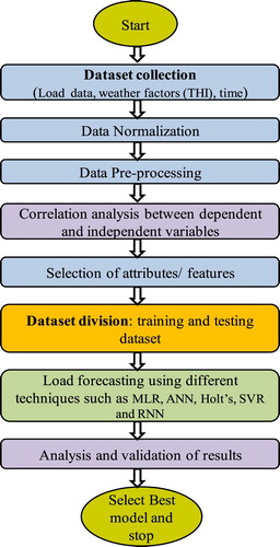
To compute the relationship between the dependent variable (load) and the independent variables (i.e. weather factors, time, etc.) and to select the variables that affect the load significantly, correlation analysis is performed. Load at any node is highly dependent on weather parameters like THI, time, and day, as a load of weekends is less as compared to the weekday loads. Therefore, these features are considered to be important attributes for training the load forecasting model. The complete dataset is divided into two parts: training and testing datasets. Subsequently, different classical and modern load forecasting techniques are used to predict the load at different nodes inside the campus. Finally, the MAPE and RMSE values are calculated by comparing the forecasted load and the actual load from each method to select the best model with minimum error values.

3.1. Load forecasting methods

Different statistical/conventional techniques are applied along with the modern/ intelligent techniques to forecast the loads at two different nodes as described below.

3.1.1. Multiple linear regression (MLR)

Multiple linear regression describes the relationship between the independent variable such as weather components like temperature, humidity, etc., and the dependent variable i.e. load. The relation between the independent variable and the dependent variable can be represented as: (2) $\tilde{y}={\beta }_0+{\beta }_1{x}_1+{\beta }_2{x}_2+\dots \dots \dots ..+{\beta }_n{x}_n+\epsilon$(2) Where;$\tilde{y}$is the dependent variable, $x_1,x_2,\dots ..$ and $x_n$ are the independent variables or input variables used to predict the dependent variable i.e. load, $\beta$ is regression coefficients and $\epsilon$ is represented as an error term (Alex and Timothy 1990). For multiple observations, we can write: ${\tilde{y}}_1={\beta }_0+{\beta }_1{x}_{11}+{\beta }_2{x}_{12}+\dots \dots \dots ..+{\beta }_k{x}_{1k}+\epsilon$ ${\tilde{y}}_2={\beta }_0+{\beta }_1{x}_{21}+{\beta }_2{x}_{22}+\dots \dots \dots ..+{\beta }_k{x}_{2k}+\epsilon$ ${\tilde{y}}_n={\beta }_0+{\beta }_1{x}_{n1}+{\beta }_2{x}_{n2}+\dots \dots \dots ..+{\beta }_k{x}_{nk}+\epsilon$

In general form, the equation can be written as: (3) ${\tilde{y}}_i={\beta }_0+\sum _{i=1}^n{\beta }_i{x}_i+\epsilon$(3)

The main goal of MLR is to develop a function that closely relates these variables so that the dependent variable can be forecasted from the values of independent variables. The basic problem is that using this method gives a linear forecasting model but the load pattern is generally a nonlinear function.

3.1.2. Artificial neural network (ANN)

ANN is a modern computational machine learning technique often used for forecasting loads that reveals certain performance characteristics resembling biological NN with the capability of parallel processing like a human brain. One major advantage of ANN is that it can be used to model any type of nonlinear multivariate function (Taylor and Buizza 2002). This method is suitable for the problems where it is difficult to specify the entire knowledge required for the solution but the number of observations is quite high. In this paper, a sigmoid activation function is used for artificial neurons. The neural network is trained using the Levenberg- Marquardt (LM) and Bayesian Regularisation (BR) algorithm by varying the number of neurons from 1 to 10 in one hidden layer. The comparative study is prepared between LM and BR algorithms to develop the ANN architecture that results in a minimum mean absolute percentage error in forecasting the load. One major drawback is that it is very tough to decide whether the derived NN is the best possible solution since it is a tiresome hit and trial process and the obtained model may get over-fitted which results in less forecasting accuracy (Hippert, Pereira, and Souza 2001).

3.1.3. Holt’s exponential smoothening method

Holt’s double parameter smoothening is a univariate method which deals with the data series having a trend. The method is based upon two smoothening equations, one for the level component and the other for the trend component which can be given as (Gob, Lurz, and Pievatolo 2013): (4) $\mathrm{Level}:A_t=\alpha \times y_t+(1-\alpha )\times (A_{t-1}+T_{t-1})$(4) (5) $\mathrm{Trend}:T_t=\beta \times (A_t-A_{t-1})+(1-\beta )\times T_{t-1}$(5)

The forecast equation can be written as: (6) $\mathrm{Forecast}:F_{t+m}=A_t+T_t\times m$(6)

The initial value of the level and trend component can be found out by the following equation: (7) $A_1=y_1,T_1={\displaystyle \frac{((y_2-y_1)+(y_4-y_3))}{2}}$(7) Where $\alpha$ and $\beta$ are smoothening constants; $A_t$ is the level component; $T_t$ is the trend component; $y_t$ is the actual load; $t$ is the time period; $F_{t+m}$ is the forecasted load for m periods ahead.

$\alpha$ is the smoothening parameter that represents weighting and the range of $\alpha$ is [0, 1]. $\beta$ is the smoothening coefficient that represents the trend component of the dataset.$\beta$ also lies in the range [0, 1]. Value of $\beta$ closer to 1 signifies that more weight is given to recent observations.

3.1.4. Support vector regression (SVR)

Support vector machine (SVM) is a powerful machine learning tool based on supervised learning for classification and regression analysis which is named SVC and SVR. SVR is a non-parametric technique as it relies on the kernel function. The kernel is a way of calculating the dot product of two vectors in a very high dimensional feature space, and the kernel function is a function used to map lower-dimensional data into higher dimensional data (Zhang, Wang, and Zhang 2017). The kernel can be linear, polynomial, and radial basis function (RBF) or Gaussian kernel. The choice of kernel function depends on the type of dataset used for modeling. In this work, a polynomial kernel is used to train the model, since the data used is highly nonlinear. The polynomial kernel is defined by Equation (8) as: (8) $K(x,y)=(c+x^{T}y{)}^n$(8) Where; n is the degree of the polynomial and c is the constant term (Zhang, Wang, and Zhang 2017).

3.2. Forecasting performance

The forecast accuracy is determined by using MAPE which is a common metric used in the field of load forecasting. It is calculated as: (9) $MAPE={\displaystyle \frac{1}{N}\left|\sum _{i=1}^N{\displaystyle \frac{(y_i-{\tilde{y}}_i)}{y_i}}\right|\times 100}$(9) Where; $y_i$ is the actual load, and ${\tilde{y}}_i$ is the forecasted load, N is the number of samples used for testing.

The root mean square error (RMSE) between actual and predicted load is calculated as: (10) $RMSE=\sqrt{{\displaystyle \frac{{\sum }_{i=1}^N{(y_i-{\tilde{y}}_i)}^2}{N}}}$(10)

4. Case study – NIT Patna campus

Smart meters are installed at 15 different nodes inside the NIT Patna campus which gives real-time data via the cloud. At any node, all the different parameters of the load data e.g. active power, reactive power, line and phase voltages, phase angle, frequency, power factor, etc. can be accessed at the desired time interval varying from 5 minutes to several hours as required.

4.1. Dataset description

For load forecasting, various combinations of load datasets used are: (a) daily average load at two different nodes for six months period ranging from 15th July 2018 to 15th January 2019, (b) hourly load at a node for six months, (c) daily load at a particular hour (10 am) for three months, (d) daily average load of the weekend for six months. These load datasets of different time horizons are used for forecasting the load at two different nodes namely Girl’s Hostel (GH) node consisting of mixed (residential+ academic+ health center) load and Incomer transformer (IT) load. The corresponding weather variables such as temperature and humidity which have a considerable effect on the load have been taken from the meteorological department. A sample dataset of daily average weekend load for both the mentioned nodes has been shown in Table 1. From the table, it can be seen that a load of September is more as compared to the load in December and January for both the nodes. The 0 value of the load at any instant may be due to the communication link failure of the smart metering device. The actual load curve of the two nodes for six months period along with the corresponding temperature and humidity is shown in Figure 2. The influence of THI on the load is analysed by the correlation analysis done in the next section.

Figure 2. A plot of (a) humidity, (b) temperature, (c) daily load of GH node, (d) daily load of IT node for six months period.

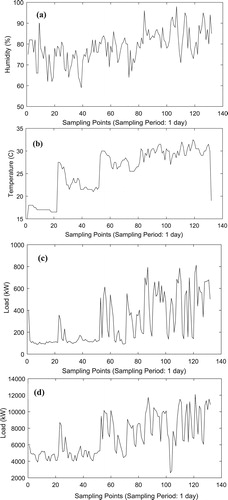
Table 1. Weekend dataset from August 2018 to January 2019

Date	Temperature (°C)	Humidity (%)	Load (Girls hostel) (kW)	Load (Incomer transformer) (kW)
5/1/19	16.00	86.00	147.92	4559.24
6/1/19	16.50	74.00	151.60	4389.12
12/1/19	16.00	75.00	416.08	5809.6
13/1/19	16.50	65.00	417.60	5080.83
19/1/19	16.50	89.00	386.88	5187.97
20/1/19	17.00	79.00	368.32	5058.49
26/1/19	19.00	92.00	17.28	5714.81
27/1/19	18.50	86.00	0.00	5895.68
1/12/18	19.00	83.00	122.56	5011.58
2/12/18	19.00	73.00	116.00	4307.65
8/12/18	18.00	75.00	125.52	4797.5
9/12/18	18.00	76.00	102.64	4168.45
15/12/18	17.50	82.00	101.28	5207.62
16/12/18	17.50	66.00	88.56	4636.87
22/12/18	17.00	79.00	91.04	4108.35
23/12/18	17.00	72.00	112.56	4083.59
29/12/18	16.50	78.00	111.28	5220.42
30/12/18	16.50	74.00	112.56	6955.65
3/11/18	27.00	81.00	140.80	4968
4/11/18	26.00	79.00	122.24	4130.88
10/11/18	22.50	70.00	103.76	5850.43
11/11/18	23.00	75.00	97.04	4699.52
17/11/18	21.50	59.00	160.88	4474.43
18/11/18	21.50	72.00	126.88	4193.22
24/11/18	21.50	76.00	115.12	5269
25/11/18	21.50	82.00	110.56	9458.69
6/10/18	29.00	81.00	219.92	8280.38
7/10/18	29.00	69.00	155.04	5373.95
13/10/18	27.50	82.00	123.76	4453.95
14/10/18	27.50	79.00	108.64	4558.79
20/10/18	28.00	83.00	92.00	8346.75
21/10/18	28.50	80.00	99.28	6041.22
27/10/18	25.50	71.00	147.68	6449.98
28/10/19	26.00	75.00	148.16	6050.05
1/9/18	30.50	83.00	226.96	10493.25
2/9/18	30.00	80.00	192.48	7373.57
8/9/18	30.00	83.00	220.16	9415.17
9/9/18	30.50	84.00	163.12	6688.52
15/9/18	31.00	79.00	471.60	5944.38
16/9/18	31.50	78.00	470.08	4092.35
22/9/18	29.50	88.00	184.48	7288.32
23/9/18	30.00	85.00	134.16	6696.52
29/9/18	30.00	79.00	181.44	11132.35
30/9/18	30.00	82.00	136.72	9171.96

4.2. Correlation analysis

Before performing regression, correlation analysis is performed to check the relation between the dependent variable (load) and the independent variables (weather variables). The correlation coefficients obtained are tabulated in Table 2. Column 1, 2, 3, and 4 represents temperature, humidity, load (girls hostel) and load (incomer transformer) respectively. From the obtained Pearson correlation coefficients, it is observed that both the temperature and humidity are closely correlated with the load as the correlation coefficients for both temperature and humidity are very high for both the nodes. It can be also said that both the loads are closely correlated to each other.

Table 2. Correlation of weather data with load

	Column 1	Column 2	Column 3	Column 4
Column 1	1
Column 2	0.935707	1
Column 3	0.811387	0.960388	1
Column 4	0.833228	0.914292	0.912617	1

From Figure 2, it can be observed that the load at both the nodes strongly follow the temperature and humidity pattern.

4.3. Data pre-processing

The data obtained directly from smart meters contain errors such as noise, communication link errors, wrong or duplicate data, etc, and this data used for load forecasting may contain some abnormality. The abnormal data should be filtered out from the entire dataset to get accurate and reliable forecasts. 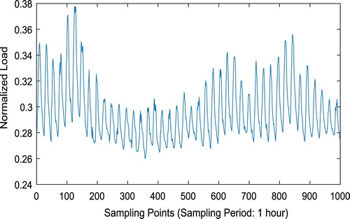The abnormal data is first normalized using the min–max normalization technique (as given in Equation (1(1) $x_{new}={\displaystyle \frac{x-x_{min}}{x_{max}-x_{min}}}$(1) )) and then filtered using a Gaussian filter. Gaussian filter is a low pass filter whose effectiveness can be controlled by adjusting the width of the filter known as preset window length. The window calculates the mean of the data points and then move one step down and again calculates the mean. This procedure is repeated until the complete data have been covered. The window length is selected after the iterative evaluation to get the best forecasting performance, and here, the selected length is 2. The processed data is then used for building the load forecasting model using different techniques. Gaussian filter is isotropic, i.e. the standard deviation is the same along both the dimensions and the Fourier transform is a Gaussian distribution centered around zero frequency. It is mainly used to reduce noise from the time series data. Figures 3 and 4 present the hourly load curve of the GH node before and after data pre-processing. These figures show the pre-processing has maintained the trend in data while enclosing variation in its magnitude within a tight range that enables improved forecasting.

Figure 3. Actual load curve of GH node

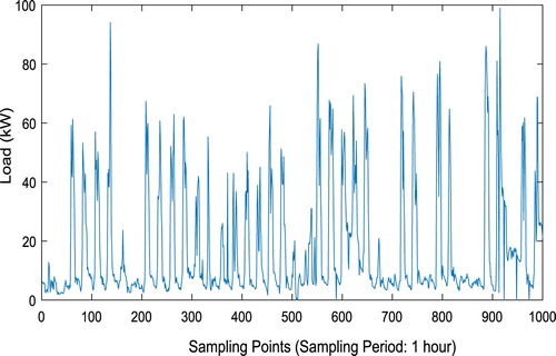
Figure 4. Load curve of GH node after pre-processing

5. Results and discussion

The smart metered data obtained from the NIT Patna campus is used for building the forecast models. Here, the daily average data for six months, hourly data for six months, and weekend and weekdays data for six months at two different nodes have been considered for analysis. 80% of the total dataset is used for training and the remaining 20% is used for testing and validating the model.

5.1. Load forecasting using different classical and machine learning techniques

Table 3 presents the MAPE and RMSE obtained for different input datasets by using the MLR technique. The feed-forward neural network is used for load forecasting in all the different testing scenarios. The algorithms that are used for training the neural network are Levenberg-Marquardt (LM) and Bayesian Regularisation (BR) algorithms. One hidden layer is used for the study and the number of neurons is varied from 5 to 100. Here, 80% of the total dataset is used for training the neural network, 10% is used for testing and the remaining 10% is used for validation of the model.

Table 3. Results of load forecast using MLR

S. No.	Cases	MAPE	RMSE
1.	Six months daily data as input for girls hostel	3.64	0.0297
2.	Six months daily data as input for incomer transformer	6.16	0.0607
4.	Six months weekend data as input for girls hostel	4.42	0.0307
5.	Six months weekend data as input for incomer transformer	5.35	0.0452
6.	Three months data at 10.a.m. as input for girls hostel	7.13	0.055

Table 4 shows the performance of ANN for six months’ daily average load at two nodes (girls hostel and incomer transformer) and three months load at a particular hour for one node (girls hostel) respectively. The regression plot for six months’ daily average load and weekend load as input dataset for girls hostel node is shown in Figures 5 and 6. From both the plots it can be seen that the regression coefficient (R-value) is very close to 1 for both the training and testing datasets. This means that the model is well trained and the actual and predicted values are highly correlated to each other, resulting in good forecasting performance.

Figure 5. Regression plot for six months daily average load of GH node

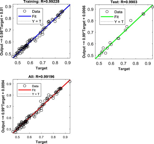
Figure 6. Regression plot for six months weekend load of GH node.

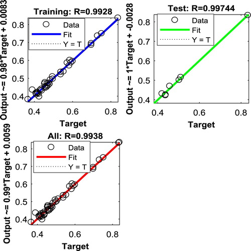
Table 4. Performance of ANN for six months daily average load

S. No	Cases	No. of neurons	MAPE	RMSE
1	Six months daily average load of GH	2 5 10	2.85 4.39 4.51	0.0245 0.0378 0.042
2	Six months daily average load of Incomer transformer	2 5 10	3.91 3.10 3.16	0.048 0.029 0.028
3	Weekend load of GH	2 5 10	4.55 5.83 5.09	0.038 0.048 0.047
4	Weekend load of Incomer transformer	2 5 10	4.35 5.63 5.07	0.034 0.043 0.047
5	Hourly load of GH at 10 am	2 5 10	2.66 2.32 2.75	0.012 0.012 0.014
6	Six months hourly load of GH	2 5 10	0.18 0.24 0.09	0.0023 0.0037 0.0021

Holt’s double exponential smoothening method is used for load forecasting. The related equations are presented in (3) and (4). The input dataset used for STLF is daily average load data of six months for two nodes, an hourly load of six months for one node, and a weekend load for six months at two nodes. In this method, the forecasting contains two components namely level and trend components as given in (3) and (4). The total forecasted load is the sum of the level and trend components. The values of level and trend constants, known as $\alpha$ and $\beta$, are initially taken as 0.5 each for forecasting and the corresponding MAPE and RMSE values are calculated. To improve the forecasting error the values of $\alpha$ and $\beta$ are optimised (between 0 to1) to get the minimum MAPE error. The objective function is given below: $MinimizeMAPE(\alpha ,\beta )={\displaystyle \frac{1}{N}\left|\sum _{i=1}^N{\displaystyle \frac{(y_i-{\tilde{y}}_i)}{y_i}}\right|\times 100}$Where y values can be found using (5) and (6). Generalised Reduced Gradient (GRG) nonlinear solver is used in this work for optimisation. The range of the coefficients alpha and beta is given 0 and 1. Initially, the solver calculates the MAPE value by taking alpha and beta as 0.5 (which is the initial set value by default). The GRG nonlinear solver calculates the slope of the objective function as the input values change and determine that it has reached the optimum solution when the partial derivatives equal to 0. Finally, it calculates the optimum value of coefficients $\alpha$ and $\beta$ for which the MAPE is minimised. In Table 5 the optimised values of $\alpha$ and $\beta$ and the corresponding minimum MAPE and RMSE for different input datasets are given. Non-linear SVR with the polynomial kernel is used to forecast the load at two given nodes under different training and testing datasets. The kernel function transforms the data into a higher dimensional feature space so that the linear separation can be done.

Table 5. Optimised values of $\alpha$ and $\beta$ for different cases with respective MAPE and RMSE values.

S. No.	Case	Value of $\alpha$	Value of $\beta$	MAPE	RMSE
1.	Six months daily average load of girls hostel	0.397	0.558	16.51	0.091
2.	Six months daily average load of incomer transformer	0.668	0.256	9.91	0.0479
3.	Six months weekend load of girls hostel	0.693	0.472	15.95	0.0409
4.	Six months weekend load of incomer transformer	0.797	0.255	3.38	0.0258
5.	Three months load data at 10 am for girls hostel	0.602	0.0803	6.89	0.0554
6.	Six months hourly load of girls hostel	0.1423	0.0472	25.42	0.0425

The polynomial kernel not only considers the given attributes of input samples to discover the similarities but also their combinations known as interactive features. Here, the order of the polynomial is varied from 1 to 5 and the corresponding MAPE and RMSE values are calculated as given in Table 6.

Table 6. Results of load forecast using SVR

S. No	Cases	Order	MAPE	RMSE
1	Six months daily average load of GH	1 2 5	3.79 3.83 4.84	0.0307 0.0299 0.0399
2	Six months daily average load of Incomer transformer	1 2 5	3.15 3.65 4.73	0.0288 0.0390 0.0691
3	Weekend load of GH	1 2 5	4.02 6.07 3.76	0.0283 0.0741 0.0289
4	Weekend load of Incomer transformer	1 2 5	4.02 6.07 3.76	0.0283 0.0741 0.0289
5	Hourly load of GH at 10 am	1 2 5	7.66 3.44 2.72	0.0329 0.016 0.013
6	Six months hourly load of GH	1 2 5	2.81 1.60 5.43	0.0031 0.0018 0.0070

5.2. Comparison of different load forecasting methods

The comparison of the results of forecasting by the above-mentioned methods is presented in Table 7. From the table, it can be seen that the MAPE calculated by the MLR method for different input datasets is in the range of 0.5% to 7%. By the ANN method, the MAPE is obtained from 0.18% to 5%. Holt’s double exponential smoothening method with the optimised value of $\alpha$ and $\beta$ yields the MAPE around 3% to 9% for three cases and has a high MAPE value for rest as given in Table 7. SVR yields a low forecasting error in all the cases as the range of error lies from 1% to 5%. From the above discussion, it can be concluded that the SVR method gives the minimum MAPE and RMSE for the residential academic load of the NIT Patna campus system with smart metering data compared to the other classical and machine learning methods described above. However, RNN is an effective method for time series forecasting in recent years as it uses its own predicted output as a training input for future prediction. Therefore, to test the superiority of the proposed SVR method, the MAPE obtained by the proposed method is compared with the MAPE obtained by RNN for all the six cases as given in Table 7. The forecasting results show that in this work the SVR method yielded a better forecast than RNN. This might be on account of the erroneous data obtained from the smart meters used for data collection in real-time. The study also suggests these regression methods heavily depend upon the nature of recorded data.

Table 7. MAPE for different forecast methods applied for various datasets

S. No	Input datasets	MAPE for different methods
		MLR	ANN	Holt’s	SVR	RNN (Zhang, Yu, and Xu 2020; de Andrade et al. 2014)
1.	Six months daily average load of girls hostel	3.64	3.91	16.51	3.83	12.49
2.	Six months daily average load of incomer transformer	6.16	3.39	9.91	3.65	8.03
3.	Six months weekend load of girls hostel	4.42	5.15	15.95	5.04	17.20
4.	Six months weekend load of incomer transformer	5.35	5.01	3.38	3.76	5.36
5.	Three months load data at 10 am for girls hostel	7.13	2.57	6.89	3.76	6.37
6.	Six months hourly load of girls hostel	0.52	0.18	25.12	1.60	15.20

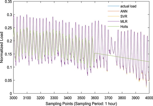
The comparison plot between actual and predicted load for different datasets using various techniques are shown in Figures 7–12.

Figure 7. Comparison plot for six months daily average load of Girls hostel.

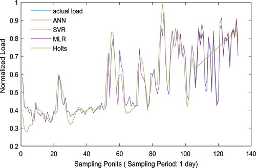
Figure 8. Comparison plot for six months daily average load of incomer transformer.

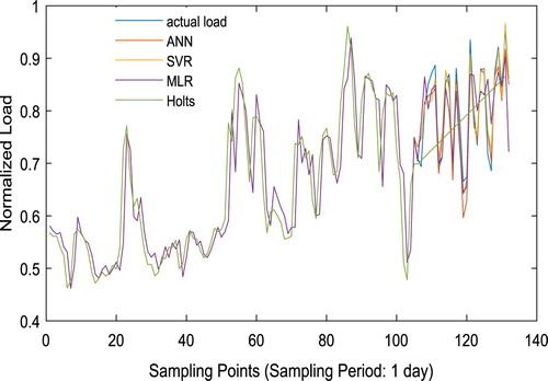
Figure 9. Comparison plot for a weekend load of Girls hostel.

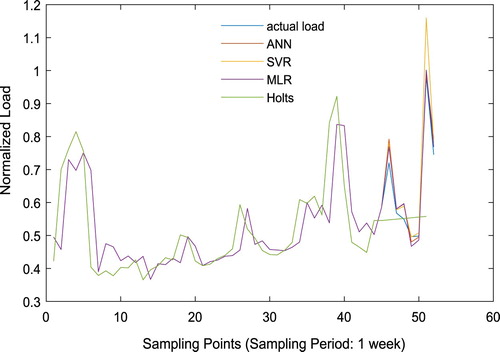
Figure 10. Comparison plot for a weekend load of incomer transformer.

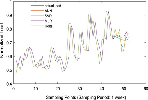
Figure 11. Comparison plot for hourly load at 10 am of Girls hostel.

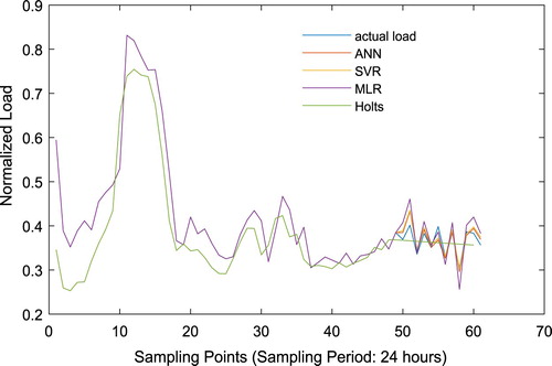
Figure 12. Comparison plot for six months hourly load of Girls hostel.

Also, the proposed result is compared with the other similar studies and the results are tabulated in Table 8. This comparative study shows that the proposed SVR method outperforms the recent works (Yildiz, Bilbao, and Sproul 2017; Solyali 2020). In addition to this, the other forecasting methods presented in this work (MLR, ANN, and Holt’s) are either better or comparative as far as the MAPE is concerned. On the contrary, it is observed that the MAPE obtained in (Moon et al. 2018) is relatively less than that of the proposed work. This may be on account of double-stage analysis in the existing work (Moon et al. 2018). Therefore, further research may be carried out in a direction in which multistage forecasting methods are implemented for better results.

Table 8. MAPE obtained with the proposed method compared with other similar studies.

Methods	Proposed	Yildiz, Bilbao, and Sproul (2017)	Solyali (2020)	Shukur et al. (2014)	Moon et al. (2018)
MLR	4.53	5.50	13.40	–	5.40
ANN	3.65	4.60	5.28	7.85	2.96
Holt’s	12.96	–	–	12.17	–
SVR	3.60	5.42	4.49	–	3.17

6. Conclusion

This paper presents multiple STLF and MTLF methods and their performance analysis using smart metered data. The forecasting is done using statistical techniques like MLR and Holt’s exponential smoothening method along with the machine learning-based approaches like ANN and SVR. Data pre-processing using Gaussian filter is used to get rid of the erroneous data or missing data which is a very common phenomenon in the case of a smart metering system due to communication failure. The suitability of the proposed method is validated through the broad comparison studies on the dataset available at the NIT Patna campus. It was found that the SVR method provides the best load forecasting for both STLF and MTLF which can be verified from the least values of MAPE and RMSE for all the testing scenarios. The average MAPE and RMSE obtained by the SVR model for all test datasets are 3.06% and 0.025 respectively, which shows that the proposed model gives very accurate and consistent load forecasting performance. Comparison with other similar studies shows that the proposed work yields better forecasting performance. The same work can be extended for a long term load forecasting which has not been done due to the unavailability of long-term training data for the used system. Additionally, the analysis with a large scale dataset for long term forecasting would attract big data analytics and introduce more complexities. Nevertheless, the methodology adopted in this work has given satisfactory load forecasting performance for short-term and mid-term analysis.

Acknowledgements

This work is supported by the Science & Engineering Research Board, a statutory body of the Department of Science and Technology (DST), Government of India, under grants number ECR/2017/001027.

Disclosure statement

No potential conflict of interest was reported by the author(s).

Additional information

Funding

This work was supported by Science and Engineering Research Board [grant number ECR/2017/001027].

References

- Aghajani, G., and N. Ghadimi. 2018. “Multi-Objective Energy Management in a Micro-Grid.” Energy Reports 4: 218–225. doi:https://doi.org/10.1016/j.egyr.2017.10.002.
- Akbary, P., M. Ghiasi, M. R. R. Pourkheranjani, H. Alipour, and N. Ghadimi. 2019. “Extracting Appropriate Nodal Marginal Prices for All Types of Committed Reserve.” Computational Economics 53 (1): 1–26. doi:https://doi.org/10.1007/s10614-017-9716-2.
- Alex, D., and C. Timothy. 1990. “A Regression-Based Approach to Short Term System Load Forecasting.” IEEE Transactions on Power Systems. 5 (4): 1535–1550.
- Aly Hamed, H. H. 2020. “A Proposed Intelligent Short-Term Load Forecasting Hybrid Models of ANN, WNN and KF Based on Clustering Techniques for Smart Grid.” Electric Power Systems Research 182.
- Amara, F., K. Agbossou, Y. Dube, S. Kelouwani, A. Cardenas, and S. S. Hosseini. 2019. “A Residual Load Modeling Approach for Household Short-Term Load Forecasting Application.” Energy and Buildings 187: 132–143.
- Brka, A., Y. M. Al-Abdeli, and G. Kothapalli. 2016. “Influence of Neural Network Training Parameters on Short-Term Wind Forecasting.” International Journal of Sustainable Energy 35 (2): 115–131. doi:https://doi.org/10.1080/14786451.2013.873437.
- de Andrade, L. C. M., M. Oleskovicz, A. Q. Santos, D. V. Coury, and R. A. S. Fernandes. 2014. “Very Short-Term Load Forecasting Based on NARX Recurrent Neural Networks.” In 2014 IEEE PES General Meeting Conference Exposition, 1–5. doi: https://doi.org/10.1109/PESGM.2014.6939012.
- Deihimi, A., O. Orang, and H. Showkati. 2013. “Short-Term Electric Load and Temperature Forecasting Using Wavelet Echo State Networks with Neural Reconstruction.” Energy 57 (4): 382–401.
- Filho, K. N., A. D. P. Lotufo, and C. R. Minussi. Oct. 2011. “Multinodal Load Forecasting Using a General Regression Neural Network.” IEEE Transactions on Power Delivery 26 (4): 2862–2869.
- Gob, R., K. Lurz, and A. Pievatolo. 2013. “Electrical Load Forecasting by Exponential Smoothing with Covariates.” Applied Stochastic Models in Business and Industry 29 (6): 629–645.
- Hagan, M. T., and S. M. Behr. August 1987. “The Time Series Approach to Short Term Load Forecasting.” IEEE Transactions of Power Systems. 2 (3). https://doi.org/10.1109/TPWRS.1987.4335210.
- Hamian, M., A. Darvishan, M. Hosseinzadeh, M. J. Lariche, N. Ghadimi, and A. Nouri. 2018. “A Framework to Expedite Joint Energy-Reserve Payment Cost Minimization Using a Custom-Designed Method Based on Mixed Integer Genetic Algorithm.” Engineering Applications of Artificial Intelligence 72: 203–212. doi:https://doi.org/10.1016/j.engappai.2018.03.022.
- Haque, A. U., P. Mandal, J. Meng, and M. Negnevitsky. 2015. “Wind Speed Forecast Model for Wind Farm Based on a Hybrid Machine Learning Algorithm.” International Journal of Sustainable Energy 34 (1): 38–51.
- Hernandez, L., C. Baladron, J. M. AguiarCarro, B. Sanchez-Esguevillas, A. J. Lloret, and J. Massana. 2014. “A Survey on Electric Power Demand Forecasting: Future Trends in Smart Grids, Microgrids, and Smart Buildings.” IEEE Communications Surveys and Tutorial 16: 1460–1495.
- Hippert, H. S., C. E. Pereira, and R. C. Souza. 2001. “Neural Network for Short Term Load Forecasting: A Review and Evaluation.” IEEE Trans. on Power Syst 16 (1): 44–55.
- Ji, P. R., D. Xiong, P. Wang, and J. Chen. 2012. “A Study on Exponential Smoothing Model for Load Forecasting.” In Proceedings of 2012 Power and Energy Eng. Conf. (APPEEC), Shanghai, China, 1–4.
- Kazantzidis, A., E. Nikitidou, V. Salamalikis, P. Tzoumanikas, and A. Zagouras. 2018. “New Challenges in Solar Energy Resource and Forecasting in Greece.” International Journal of Sustainable Energy 37 (5): 428–435.
- Kleebrang, W., P. Bunditsakulchai, and W. Wangjiraniran. 2017. “Household Electricity Demand Forecast and Energy Savings Potential for Vientiane, Lao PDR.” International Journal of Sustainable Energy 36 (4): 344–367. doi:https://doi.org/10.1080/14786451.2015.1017501.
- Leng, H., X. Li, J. Zhu, H. Tang, Z. Zhang, and N. Ghadimi. 2018. “A New Wind Power Prediction Method Based on Ridgelet Transforms, Hybrid Feature Selection and Closed-Loop Forecasting.” Advanced Engineering Informatics 36: 20–30.
- Liao, G. C., and T. P. Tsao. 2006. “Application of a Fuzzy Neural Network Combined with a Chaos Genetic Algorithm and Simulated Annealing to Short-Term Load Forecasting.” IEEE Transactions on Evolutionary Computation 10 (3): 330–340.
- Liu, Y., W. Wang, and N. Ghadimi. 2017. “Electricity Load Forecasting by an Improved Forecast Engine for Building Level Consumers.” Energy 139: 18–30. doi:https://doi.org/10.1016/j.energy.2017.07.150.
- Mirzapour, F., M. Lakzaei, G. Varamini, M. Teimourian, and N. Ghadimi. 2019. “A New Prediction Model of Battery and Wind-Solar Output in Hybrid Power System.” Journal of Ambient Intelligence and Humanized Computing 10 (1): 77–87.
- Moghram, I., and S. Rahman. 1989. “Analysis and Evaluation of Five Short-Term Load Forecasting Techniques.” IEEE Trans. Power Systems 4 (4): 1484–1491.
- Moon, J., K. Kim, Y. Kim, and E. Hwang. 2018. “A Short-Term Electric Load Forecasting Scheme Using 2-Stage Predictive Analytics.” In 2018 IEEE International Conference on Big Data and Smart Computing (BigComp), 219–226.
- Moshkbar-Bakhshayesh, K., and M. B. Ghofrani. 2014. “Development of a Robust Identifier for NPPs Transients Combining ARIMA Model and EBP Algorithm.” IEEE Transactions on Nuclear Science 61 (4): 2383–2391.
- Nazar, M. S., A. E. Fard, A. Heidari, M. S. Khah, and J. P. S. Catalao. 2018. “Hybrid Model Using Three-Stage Algorithm for Simultaneous Load and Price Forecasting.” Electrical Power System Research 165: 214–228.
- Rahman, S., and I. Drezga. 1992. “Identification of a Standard for Comparing Short-Term Load Forecasting Techniques.” Electric Power Systems Research 25 (3): 149–158.
- Salim, O. M., M. A. Zohdy, H. T. Dorrah, and A. M. Kamel. 2014. “Adaptive Neuro-Fuzzy Short-Term Wind-Speed Forecasting for Egypt’s East-Coast.” International Journal of Sustainable Energy 33 (1): 16–34. doi:https://doi.org/10.1080/14786451.2011.630468.
- Shukur, O., N. Fadhil, M. H. Lee, and M. Ahmad. 2014. “Electricity Load Forecasting Using Hybrid of Multiplicative Double Seasonal Exponential Smoothing Model with Artificial Neural Network.” Jurnal Teknologi 69, doi:https://doi.org/10.11113/jt.v69.3109.
- Solyali, D. 2020. “A Comparative Analysis of Machine Learning Approaches for Short-/Long-Term Electricity Load Forecasting in Cyprus.” Sustainability 12 (9), doi:https://doi.org/10.3390/su12093612.
- Taylor, J. W., and R. Buizza. 2002. “Neural Network Load Forecasting with Weather Ensemble Predictions.” IEEE Transactions on Power Systems 17 (3): 626–632.
- Taylor, J. W., and P. E. McSharry. 2007. “Short-Term Load Forecasting Methods: Evaluation Based on European Data.” IEEE Transactions on Power Systems 22 (4): 2213–2219.
- Tian, C., J. Ma, C. Zhang, and P. Zhan. 2018. “A Deep Neural Network for Short-Term Load Forecast Based on LSTM and Conv. Neural Network.” Energies 11: 3493.
- Wang, Y., Q. Chen, T. Hong, and C. Kang. 2018. “Review of Smart Meter Data Analytics: Applications, Methodologies, and Challenges.” IEEE Transactions on Smart Grid.
- Wen, L., K. Zhou, and S. Yang. 2020. “Load Demand Forecasting of Residential Buildings Using a Deep Learning Model.” Electric Power Systems Research 179: p. 106073. doi:10.1016/j.epsr.2019.106073.
- Xiao, Z., S. Ye, Bo Zhong, and C. Sun. 2009. “BP Neural Network with Rough Set for Short Term Load Forecasting.” Expert Systems With Applications 36 (1): 273–279.
- Yildiz, B., J. I. Bilbao, and A. B. Sproul. 2017. “A Review and Analysis of Regression and Machine Learning Models on Commercial Building Electricity Load Forecasting.” Renewable and Sustainable Energy Reviews 73: 1104–1122. doi:https://doi.org/10.1016/j.rser.2017.02.023.
- Zhang, X., J. Wang, and K. Zhang. 2017. “Short-Term Electric Load Forecasting Based on Singular Spectrum Analysis and Support Vector Machine Optimized by Cuckoo Search Algorithm.” Electric Power Systems and Research 146: 270–285.
- Zhang, P., X. Wu, and X. Wang. September 2015. “Short-Term Load Forecasting Based on Big Data Technologies.” CSEE Journal of Power and Energy Systems 1 (3): 59–67.
- Zhang, M., Z. Yu, and Z. Xu. 2020. “Short-Term Load Forecasting Using Recurrent Neural Networks With Input Attention Mechanism and Hidden Connection Mechanism.” IEEE Access 8: 186514–186529. doi:https://doi.org/10.1109/ACCESS.2020.3029224.