Estimation of daylight availability in Kolkata and approximation of indoor daylight levels for different daylighting methods

ABSTRACT

This work estimated the daylight availability and luminous efficacy of solar illuminance and approximated indoor daylight levels for various indoor daylighting methods for Kolkata, a major city in eastern India having tropical savanna climate, by applying two computational methods: the Perez model and the IESNA recommended calculation procedure. It was found that hourly horizontal diffuse and global illuminance, horizontal sky and total daylight illuminance values remained mostly over 10 klx throughout the year, and global and diffuse luminous efficacies mostly remained around 95–120 and 110–150 lm/W, respectively. The linear correlation between solar irradiation and estimated illuminance was stronger for Perez model. Thus, the application of Perez model was considered the better choice to appraise the daylighting potential of Kolkata.

KEYWORDS:

• Daylight availability
• solar illuminance
• daylighting devices
• global luminous efficacy
• diffuse luminous efficacy

1. Introduction

Solar radiation is a great source of renewable energy worldwide and an estimated four million exajoules (4 × 10⁶ EJ) of solar energy is received annually by the earth of which fifty-thousand exajoules (5 × 10⁴ EJ) could potentially be harnessed by current technology (Kabir et al. 2018). Proper utilisation of solar energy helped the human civilisation to develop and prosper through various ages. Today, harnessing its potential could have various facets in daily life and it would prove to be an advantageous choice over conventional fossil fuel-based power systems (Kalogirou 2004). It could considerably reduce global carbon emissions (Shahsavari and Akbari 2018), solar and biomass energy-based hybrid combined cooling heating and power systems (CCHP) could be driven at a greater system energy efficiency (Wang and Yang 2016), remote areas could avail basic utilities of electrification (Chakrabarti and Chakrabarti 2002) and street lighting systems could employ LEDs to efficiently utilise the stored electrical energy in battery banks, harnessed from solar radiation (Dalla Costa et al. 2010), which would advance the recent developments pertaining to energy-efficient road lighting planning that is currently focused on road classification (Chakraborty et al. 2018).

Solar energy not only can be used for electricity generation and heating but also can be used for daylighting purposes. Daylight is the ‘holistic combination’ of the luminous characteristics of sunlight and skylight (Knoop et al. 2020) and is termed as a ‘key design driver’ (Turan et al. 2020) in the commissioning of construction projects. It is of significant importance to architects and lighting designers to reduce the net electrical load associated with lamps and necessary apparatus, such as ballasts, control gears, dimmers, etc. and adaptive lighting and shading control techniques may assist efforts to reduce energy consumption in lighting systems (Bisegna et al. 2016). Extensive research works have been conducted on the minimisation of energy consumption of lamp-based electrical loads in cost-optimal nearly zero energy buildings (ZEBs) (Pikas, Thalfeldt, and Kurnitski 2014; D'Agostino and Parker 2018; Doulos et al. 2019) and daylighting is seen as a potent tool to lower the electrical energy consumption of artificial illumination systems (Okogbue, Adedokun, and Holmgren 2008) as overall requirements of illumination could be met by controlling artificial illumination systems according to available indoor daylight levels (Alrubaih et al. 2013).

Daylight is considered to be the best source of illumination for colour rendering, it can provide 110 lumens of luminous flux per Watt of solar radiation (a luminous efficacy of 110 lm/W) and its spectra closely match the human spectral visual response (Kandilli and Ulgen 2008). However, the luminous efficacy of daylight varies with sky clearness, solar altitude and atmospheric conditions. It is 70–105 lm/W for direct sunlight, approximately 130 lm/W for the clear sky and around 110 lm/W for the overcast sky under diffuse skylight (Littlefair 1985). Furthermore, daylight is a natural, temporally variant (Ferenčíková and Darula 2017), dynamic source of illumination (Deroisy and Deneyer 2017) and its spectral power distribution (SPD) for the 330 –700 nm wavelength range was measured by Henderson and Hodgkiss (1963). The CIE Standard Illuminant D65 is a hypothesised illuminant to simulate the naturally occurring standard illumination conditions under daylight and attempts have been made to design and simulate the D65 (Powell 1996; Lam and Xin 2002). Moreover, the human circadian clock is entrained to sunlight or more specifically the 24-h solar cycle (Duffy and Wright Jr 2005; Roenneberg et al. 2013; Woelders et al. 2017) and exposure to daylight assumes much importance in the everyday life of human beings since human health and wellness are intricately linked to it and various studies have indicated that daylight is preferred to artificial illumination in different settings or fields of human activity (Markus 1967; Cuttle 1983; Heerwagen and Heerwagen 1986; Galasiu and Veitch 2006).

Currently, there is an impetus on daylight integration and control in commercial buildings, residential spaces and other indoor environments (Colaco et al. 2008; Xue, Mak, and Cheung 2014; Darula 2018; Kose and Kazanasmaz 2020) and the performance of different types of windows have been evaluated, by experimentation or simulation. Fasi and Budaiwi (2015) used the ‘DesignBuilder’ computer program to simulate an office space under a hot climate and found that the building energy consumption reduced for all the types of glazing of the window models. It was further reported that automatic interior shading control achieved visual comfort and did not increase energy consumption. Kousalyadevi and Lavanya (2019) utilised the ‘Velux’ software to simulate the daylighting conditions of an industrial building and measured the energy consumption. It was found that the maximum daylight illuminance level was 902.3 lx and the energy-saving potential (ESP) could reach up to 31.4% for dimming control of artificial lighting with a top daylighting panel. Ghisi and Tinker (2005) used the ‘VisualDOE’ computer program to simulate the climatic conditions of Leeds, United Kingdom and Florianopolis, Brazil and proposed a methodology of prediction of energy savings integrating the concepts of ‘Ideal Window Area’ and ‘Daylight Factors’. Al-Ashwal and Hassan (2017) investigated the potential of energy savings by daylight integration with electrical lighting for a classroom scenario in a tropical climate using the ‘Energy Plus’ computer program. It was concluded that electrical energy consumption for artificial illumination could be reduced by 28–40% which is 10–18% of the total energy consumption. Azad, Rakshit, and Patil (2018) measured daylight in New Delhi, India and characterised global and diffuse luminous efficacy patterns. Their work compared four efficacy models and ameliorated the outputs using optimised coefficients, adopted from the measured data. Variations in global and diffuse luminous efficacy values were presented for clear, intermediate and overcast sky conditions and average monthly global and diffuse illuminance values were estimated with original and modified efficacy models. A similar work estimated global and diffuse luminous efficacy for the tropical region of Bangkok, Thailand, proposed two empirical all-weather efficacy models and validated the same (Chaiwiwatworakul and Chirarattananon 2013). Dieste-Velasco et al. (2019) compared the performance of 18 luminous efficacy models with a proposed model utilising measured global illuminance values for varied sky conditions in Burgos, Spain and concluded that the proposed model fared well under varied sky conditions. A pioneering work conducted by Bellia and Fragliasso (2017) proposed new parameters, such as Daylight Integration Adequacy, Percentage Light Deficit (PLD), Percentage Intrinsic Light Excess (PILE) and Percentage Light Waste (PLW), to analyse the performance of daylight-linked artificial illumination control systems and presented a simple case study in support of their proposition.

Nevertheless, daylight integration in artificially lit indoor environments would require careful architectural planning and availability of daylight data for all the regions in which such exercise shall be carried out. However, there is a dearth of literature on solar illuminance data for various weather stations in India and as such, estimation of solar illuminance levels should be done from meteorological data, solar insolation maps (Rao and Seshadri 1961) and predicted mean diffuse solar radiation tables (Karakoti, Das, and Singh 2012). Using the 2014 SUNY semi-empirical model solar irradiance data of National Solar Radiation Database (NSRDB), National Renewable Energy Laboratory (NREL 2014; Sengupta et al. 2018), this work estimated the solar illuminance levels of Kolkata, India (22.5726° N, 88.3639° E) with Oracle software using two computational methods: the Perez model (Perez et al. 1990) and the IESNA recommended calculation procedure of estimating daylight availability (IES Calculation Procedures Committee 1984); and compared the simulated results with results obtained from photometric measurements that were carried out in April 2020. The calculated daylight data were utilised to assess indoor daylight illuminance levels for four different daylighting devices: motorised window shading, light pipe, skylight and light shelf. The objectives of this work are to assess the consistency of simulated photometric outputs (solar illuminance levels) with measured photometric outputs, estimate indoor daylight illuminance levels for various daylighting devices, and commentate on the reliability of the two computational methods that have been used.

2. Methodology

2.1. Geographical description and collection of solar irradiation data

Daylighting of buildings requires careful consideration of daylight availability and prediction of daylight availability is dependent upon a number of factors, such as geographical location, climate, altitude, atmospheric turbidity, cloud cover and cloudscape. Kolkata, a major city in eastern India, has a tropical savanna climate and receives maximum rainfall from June to August. The winter lasts from November to February. Solar radiation data of Kolkata, obtained from the NREL database, was utilised to facilitate daylight computations. Table 1 provides a compendium of ten years (2005–2014) monthly average energy data of global horizontal irradiation (GHI), direct normal irradiation (DNI) and temperature (T), as obtained from the PVGIS-5 geo-temporal irradiation database (PVGIS 2020).

Table 1 . Ten years (2005–2014) monthly average GHI, DNI and temperature (T) for Kolkata.

Month	Unit area energy content of GHI (kWh/m^2)	Unit area energy content of DNI (kWh/m^2)	T (°C)
January	138.669	157.515	17.68
February	150.763	162.24	21.8
March	190.778	176.104	27.02
April	200.373	167.353	30.33
May	191.853	134.267	30.98
June	150.526	84.886	29.64
July	142.831	72.639	27.6
August	139.621	73.557	27.49
September	138.162	90.139	27.05
October	142.856	123.482	25.62
November	138.573	148.147	21.99
December	133.692	157.11	17.94

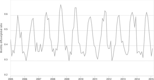
Figures 1 and 2 depict the monthly hourly average GHI and diffuse horizontal irradiation (DHI) (in W/m²) for Kolkata for the year 2014 from 7:30 am to 5:30 pm, as obtained from the NREL database and Figure 3 provides the monthly DHI to GHI ratio for the period of 2005–2015, as obtained from the PVGIS-5 geo-temporal irradiation database (PVGIS 2020).

Figure 1. Monthly hourly average GHI in Kolkata.

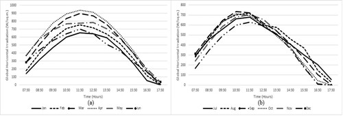
Figure 2. Monthly hourly average DHI in Kolkata.

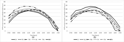
Figure 3. Monthly DHI to GHI ratio for Kolkata for the period of 2005–2015 .

2.2. The Perez model

The Perez model was proposed in 1990 and it can be used to model daylight availability from direct and global solar irradiance data (Perez et al. 1990). It has been applied and validated by researchers for estimating daylight availability for different climatic conditions (Muneer and Angus 1993; Muneer 1996; Joshi, Sawhney, and Buddhi 2007; Patil, Garg, and Kaushik 2013; Raul, Pal, and Roy 2015). Solar irradiance, dew point temperature and geographical altitude data are prerequisites of this model to compute daylight availability of any geographical region of known latitude and longitude. The calculation procedure is described below.

The global (K_g) and diffuse (K_d) luminous efficacies can be found out from the equation given herein (1) $K_{\mathrm{g}}or{K}_{\mathrm{d}}=a_i+b_{i}W+c_i\cos (z)+d_i{\log }_{\mathrm{e}}(\mathrm{\Delta })\dots$(1) where a_i, b_i, c_i and d_i are coefficients dependent upon sky clearness and are given in Table 2, W is atmospheric precipitable water content, z is the zenith angle and $\mathrm{\Delta }$ is sky brightness.

Table 2 . Global and diffuse luminous efficacy coefficients of Perez model.

Sky category	Sky clearness ($\epsilon$)		Coefficients of global luminous efficacy (Kg)				Coefficients of diffuse luminous efficacy (Kd)
	Lower limit	Upper limit	ai	bi	ci	di	ai	bi	ci	di
Overcast	1	1.065	96.63	−0.47	11.5	−9.16	97.24	−0.46	12	−8.91
	1.065	1.23	107.54	0.79	1.79	−1.19	107.22	1.15	0.59	−3.95
	1.23	1.5	98.73	0.7	4.4	−6.95	104.97	2.96	−5.53	−8.77
	1.5	1.95	92.72	0.56	8.36	−8.31	102.39	5.59	−13.95	−13.9
	1.95	2.8	86.73	0.98	7.1	−10.94	100.71	5.94	−22.75	−23.74
	2.8	4.5	88.34	1.39	6.06	−7.6	106.42	3.83	−36.15	−28.83
	4.5	6.2	78.63	1.47	4.93	−11.37	141.88	1.9	−53.24	−14.03
Clear	6.2	–	99.65	1.86	−4.46	−3.15	152.23	0.35	−45.27	−7.98

The atmospheric precipitable water content (W) is given as (2) $W=e^{(0.07T_{\mathrm{d}}-0.075)}\dots$(2) where T_d is the dew point temperature and W is given in cm (Wright, Perez, and Michalsky 1989).

Solar zenith angle (z) is calculated through the following equation (3) $\cos (z)=\cos (\phi )\ast \cos (\delta )\ast \cos (\omega )+\sin (\phi )\ast \sin (\delta )\dots$(3) where $\phi$ is the latitude of the geographical location, $\delta$ is the solar declination angle and $\omega$ is the hour angle.

Solar declination angle ($\delta$) may be calculated as (4) $\delta ={23.45}^{\circ }\sin \left({\displaystyle \frac{360(284+n)}{365}}\right)\dots$(4) where n is the date serial number of the year.

Hour angle ($\omega$) is calculated from the following formula (5) $\omega ={15}^{\circ }(\mathrm{LST}-12)\dots$(5) LST is the local solar time, dependent upon local time (LT) and is given as follows (6) $\mathrm{LST}=\mathrm{LT}+{\displaystyle \frac{4(\mathrm{Longitude}-{15}^{\circ }\ast \mathrm{\Delta }{T}_{\mathrm{UTC}})+9.87\sin (2B)-7.53\cos (B)-1.5\sin (B)}{60}\dots }$(6) B is expressed in degrees and is given as (7) $B={\displaystyle \frac{360}{365}(n-81)\dots }$(7) $\mathrm{\Delta }{T}_{\mathrm{UTC}}$ is the difference of the LT from Universal Coordinated Time in hours.

Sky clearness ($\epsilon$) is expressed as (8) $\epsilon ={\displaystyle \frac{((I_{\mathrm{d}}+I_{\mathrm{n}})/I_{\mathrm{d}})+k{z}^3}{1+k{z}^3}\dots }$(8) where I_d is the diffuse irradiance, I_n is the normal irradiance, k = 1.041 and z is the solar zenith angle in radians.

Normal irradiance (I_n) is expressed as (9) $I_{\mathrm{n}}={\displaystyle \frac{I_{\mathrm{b}}}{\cos (z)}\dots }$(9) where I_b is the beam irradiance or direct normal irradiance (DNI).

Sky brightness ($\mathrm{\Delta }$) is expressed as (10) $\mathrm{\Delta }=m{\displaystyle \frac{I_{\mathrm{d}}}{I_{\mathrm{E}}}\dots }$(10) where m is the air mass and I_E is the horizontal extra-terrestrial irradiance.

Air mass m is obtained from the following formula (Kasten 1993) (11) $m=[\sin ({\alpha }_{\mathrm{s}})+0.50572{({\alpha }_{\mathrm{s}}+6.07995)}^{-1.6364}{]}^{-1}\dots$(11) where ${\alpha }_{\mathrm{s}}$ is the solar altitude angle and it is complementary to the solar zenith angle z.

Corrected air mass (m'), taking into account the effects of air pressure, is given by (12) $m^{\mathrm{\prime }}=m\ast {\displaystyle \frac{p}{p_0}\dots }$(12) Standard atmospheric pressure p₀ is 1013.25 millibar at sea level. Atmospheric pressure p (millibar) at any height h may be determined by the following equation (13) $p=p_0{e}^{-0.0001184h}\dots$(13) The horizontal extra-terrestrial irradiance (I_E) is calculated as (Kalogirou 2014) (14) $I_{\mathrm{E}}=G_{\mathrm{SC}}\left[1+0.033\cos \left({\displaystyle \frac{360n}{365}}\right)\right]\cos (z)\dots$(14) where G_SC is the solar constant having a value of 1366.1 W/m² as per the latest adopted value of the American Society for Testing and Materials (ASTM).

Two parameters to quantify solar or more specifically daylight illumination, namely, global horizontal illuminance (E_g) and diffuse horizontal illuminance (E_d), are determined from the following two equations: (15) $E_g=I_g\ast K_g\dots$(15) (16) $E_{\mathrm{d}}=I_{\mathrm{d}}\ast K_{\mathrm{d}}\dots$(16) where I_g and I_d are mathematical notations used to denote GHI and DHI, respectively. Diffuse horizontal illuminance (E_d) values cannot exceed global horizontal illuminance (E_g) and as such, E_d values marginally exceeding E_g values, if any, should be equated to the corresponding E_g values to maintain consistency of the model.

2.3. The IESNA recommended calculation procedure of estimating daylight availability

The IESNA recommended calculation procedure of daylight availability was first published in 1984 (IES Calculation Procedures Committee 1984). It was an amelioration over earlier publications regarding this subject and it included partly cloudy sky conditions. The elementary calculation procedure is given herein.

Solar declination angle ($\delta$) is given by the following equation (17) $\delta =0.4093\sin \left[{\displaystyle \frac{2\pi }{368}(n-81)}\right]\dots$(17) where n is the day of the year ($1\le n\le 365$).

Solar altitude angle (${\alpha }_s$) may be determined from the following equation (18) ${\alpha }_{\mathrm{s}}=\arcsin \left[\sin l\ast \sin \delta -\cos l\ast \cos \delta \ast \cos {\displaystyle \frac{\pi t}{12}}\right]\dots$(18) where l is the latitude of the geographical location and t is the solar time.

The solar azimuth angle (α_az) can be found out from the following expression (19) ${\alpha }_{\mathrm{az}}=\arctan \left[{\displaystyle \frac{\cos \delta \sin {\displaystyle \frac{\pi t}{12}}}{\cos l\sin \delta +\sin l\cos \delta \cos {\displaystyle \frac{\pi t}{12}}}}\right]\dots$(19) The extra-terrestrial solar illuminance E_xt is determined from the following equation (20) $E_{\mathrm{xt}}=E_{\mathrm{SC}}\left[1+0.034\cos \left\{{\displaystyle \frac{2\pi }{365}(n-2)}\right\}\right]\dots$(20) where E_SC is the solar illumination constant at 127.5 klx.

The direct normal solar illuminance E_dn is governed by the following equation (21) $E_{\mathrm{dn}}=E_{\mathrm{xt}}\ast e^{-c\ast m}\dots$(21) where c is the atmospheric extinction coefficient as given in Table 3 and m is the optical air mass as given in the following equation (22) $m={\displaystyle \frac{1}{\sin {\alpha }_{\mathrm{s}}}\dots }$(22) The direct horizontal solar illuminance E_dH is found out from the following equation (23) $E_{\mathrm{dH}}=E_{\mathrm{dn}}\sin {\alpha }_{\mathrm{s}}\dots$(23) The horizontal sky illuminance E_kH, which can be thought to be analogous to the diffuse horizontal illuminance (E_d) term of Perez model, can be estimated from the given equation herein (24) $E_{\mathrm{kH}}=A+B\mathrm{si}{\mathrm{n}}^C({\alpha }_{\mathrm{s}})\dots$(24) where A is the ratio of sunrise to sunset illuminance, B and C are solar altitude illuminance coefficient and solar altitude illuminance exponent, respectively, and are given in Table 3.

Table 3 . Various IESNA recommended daylight availability constants.

Sky condition	Atmospheric extinction coefficient (c)	Sunrise to sunset illuminance ratio (A) in klx	Solar Altitude Illuminance Coefficient (B) in klx	Solar altitude illuminance exponent (C) in klx
Clear	0.21	0.8	15.5	0.5
Partly cloudy	0.80	0.3	45	1
Cloudy	^a	0.3	21	1

^a For no direct sun, E_dn= 0.

Now, the sky condition is divided into three types: clear, partly cloudy and cloudy. The concept of sky ratio was utilised which could take account of the atmospheric scattering of incident solar irradiation by gases, dust, water vapour and colloidal particles. Sky ratio is the ratio of diffuse horizontal (sky) irradiance to global horizontal irradiance. Table 4 provides the sky ratio ranges corresponding to the three sky conditions.

Table 4 . Sky ratio ranges corresponding to different sky conditions.

Sky condition	Sky ratio
Clear	<0.3
Partly cloudy	0.3–0.8
Cloudy	>0.8

Total daylight illuminance (E), which can be thought to be analogous to the global horizontal illuminance (E_g) term of Perez model, is the summation of direct horizontal solar illuminance and horizontal sky (diffuse) illuminance. (25) $E=E_{\mathrm{dH}}+E_{\mathrm{kH}}\dots$(25)

2.4. Measurement of solar illuminance

To validate the simulated results, solar illuminance was measured in the month of April 2020 in Kolkata, India with an unobstructed sky. The measurements were conducted every day from 7:30 am to 5:30 pm with an interval of one hour. Two digital photometers were utilised to carry out the measurements. One measured the global solar illuminance component on a surface parallel to the ground for the unabated sky dome, the other was provided with a custom-made manually operable shading ring-shaped apparatus to measure the diffuse solar illuminance on the same surface. The measured values were duly tabulated.

2.5. Estimation of indoor daylight illuminance with window shading control

The daylight transmitted through windows with installed shading devices is usually governed by the position of the sun and the prevailing conditions of the sky (Molina, Maestre, and Lindawer 2000). Control strategies and connections to electrical lighting systems of automatically controlled blinds influence electrical energy savings (Konstantoglou and Tsangrassoulis 2016). Yao (2018) developed a stochastic model to simulate daylighting with manual solar shades and found that manual solar shades could significantly increase useful daylight illuminance. A detailed methodology to calculate indoor daylight levels for office spaces with motorised blinds was provided by Athienitis and Tzempelikos (2002). The fundamental equations to calculate daylight transmittance under both clear and overcast sky conditions are given herein.

The transmittance for the overcast sky is given by the following equation (26) ${\tau }_{\nu }^{o\mathrm{vercast}}={\displaystyle \frac{4.5\ast {10}^{12}\ast {\beta }^{-6}}{e^{(335/\beta )}-1}\dots }$(26) where β is the blind tilt angle.

The transmittance for the clear sky is given by the following equation (27) $\begin{array}{rl}& {\tau }_{\nu }^{\mathrm{clear}}(\beta ,\theta )=0.55e^{-{(\beta -80)}^2/1900}\times (-4.917\times {10}^{-7}{\theta }^4+0.00009{\theta }^3-0.00567{\theta }^2+0.13\theta -0.00437)\end{array}$(27) where θ is the angle of incidence of direct sunlight on window glazing or surface.

For an overcast sky, the total daylight incident upon a window is the summation of daylight reaching from the sky and from the ground after reflection. This may be mathematically expressed as (28) $E_{\mathrm{w}}^{\mathrm{overcast}}=E_{\mathrm{h}}\ast F_{\mathrm{w}-\mathrm{sky}}+E_{\mathrm{h}}\ast F_{\mathrm{w}-\mathrm{g}}\ast {\rho }_{\mathrm{g}}\dots$(28) where E_w is the daylight incident upon a window, E_h is analogous to global horizontal illuminance or total daylight illuminance, F_w-sky is the view factor between the window and the sky (typical value 0.5), F_w-g is the view factor between the window and the ground (typical value 0.5) and ${\rho }_{\mathrm{g}}$ is the reflectance of the ground.

The daylight transmitted into the room on an overcast day may be given by the following equation (29) $E_{\mathrm{overcast}}=E_{\mathrm{h}}(F_{\mathrm{w}-\mathrm{sky}}+F_{\mathrm{w}-\mathrm{g}}\ast {\rho }_{\mathrm{g}})\ast {\tau }_{\nu }^{\mathrm{overcast}}\dots$(29) For a clear sky, the total daylight incident upon a window is the summation of daylight directly from the sun, diffuse skylight and daylight reflected from the ground. This may be mathematically expressed as (30) $E_{\mathrm{w}}^{\mathrm{clear}}=E_{\mathrm{w}-\mathrm{sun}}+F_{\mathrm{w}-\mathrm{sky}}\ast E_{\mathrm{h}-\mathrm{sky}}+E_{\mathrm{h}}\ast F_{\mathrm{w}-\mathrm{g}}\ast {\rho }_{\mathrm{g}}\dots$(30) where $E_{\mathrm{h}-\mathrm{sky}}$ is the horizontal sky (diffuse) component of daylight illuminance.

The term $E_{\mathrm{w}-\mathrm{sun}}$ is given by the following equation (31) $E_{\mathrm{wsun}}=E_0\times f(n)\times e^{-c\times m}\times \cos (\theta )\dots$(31) where E₀ is the average illuminance upon a surface, outside the atmosphere of earth, that normal to incident sunlight and its value is taken as 127,500 lx. The superscript ‘c’ is given in Table 3 and ‘m’ is given in Equation (22). The term f(n) is a correction factor that takes account of the orbital shape of the earth (ellipse). It is given by the following equation (n is day serial number) (32) $f(n)=1+0.033\cos \left({\displaystyle \frac{360n}{365}}\right)\dots$(32) The daylight transmitted into the room on a clear day may be given by the following equation (33) $E_{\mathrm{clear}}=E_{\mathrm{w}}^{\mathrm{clear}}\times {\tau }_{\nu }^{\mathrm{clear}}\dots$(33)

2.6. Estimation of indoor daylight illuminance with light pipes

Indoor daylight illumination can be achieved with the assistance of light pipes which are straight cylinders with highly reflective inner surfaces. Light pipes may help daylight penetrate into deeper spaces of buildings. Various studies have analysed the daylighting and ESP of light pipes under different climate conditions (Carter 2002; Yun, Hwang, and Kim 2010; Samuhatananon, Chirarattananon, and Chirarattananon 2011; Shin, Yun, and Kim 2012). A study (Mandal and Roy 2016) proposed an adaptive dimming scheme for a light pipe-integrated indoor lighting system that could maintain a constant workplane illuminance level. The flux confinement diagram (FCD) of rectangular light pipes was developed by Van Derlofske and Hough (2004) which could assist in designing first-order light pipe luminous flux transmission systems. However, a simplified method to determine average indoor daylight illumination for a room with ceiling mounted light pipes was provided by Maňková, Hraška, and Janak (2009) which is useful to predict indoor daylight illuminance contribution from light pipes using computed exterior daylight illuminance data. The equation for average horizontal workplane illuminance calculation is given herein (34) $E_{\mathrm{avg}}={\displaystyle \frac{n\times E_{\mathrm{g}}\times A_{\mathrm{d}}\times {\eta }_{\mathrm{t}}\times \mathrm{UF}\times \mathrm{LLF}}{A}\dots }$(34) where $n$ is the number of light pipes, $E_{\mathrm{g}}$ is the global horizontal illuminance, $A_{\mathrm{d}}$ is the area of diffuser, ${\eta }_{\mathrm{t}}$ is the tube transmission efficacy, $\mathrm{UF}$ is the utilisation factor, $\mathrm{LLF}$ is the light loss factor and A is the workplane area. Equation (34) is best suited for application with CIE standard overcast sky but it may also be applied to calculate indoor daylight illuminance for other prevailing sky conditions as well with a reasonable degree of accuracy.

2.7. Estimation of indoor daylight illuminance with skylights

Ceiling mounted skylights are a viable alternative to light pipes to introduce daylight into indoor environments. These can be also used in conjunction with light pipes. Skylights can save the electrical energy required for lighting and heating and provide a ‘natural view’ of the sky. Different studies have explored the visual and non-visual effects of the artificial skylight (Canazei et al. 2016; Canazei et al. 2017; Yasukouchi et al. 2019) and it was found that artificial skylights elevate occupants’ mood in windowless environments (Canazei et al. 2017). The ‘lumen method of skylighting’ to estimate average horizontal workplane illuminance due to skylights was elucidated by Kaufman (1981). The average horizontal workplane illuminance due to a number of skylights can be determined from the following equation for an overcast sky (Murdoch 1994) (35) $E_{\mathrm{avg}}^{\mathrm{overcast}}=E_{\mathrm{h}}\times {\displaystyle \frac{N\ast A_{\mathrm{skylight}}}{A_{\mathrm{workplane}}}\times K_{\mathrm{diffuse}}\times K_m\dots }$(35) For a day with clear sky and direct sunlight, the same can be given as follows (36) $E_{\mathrm{avg}}^{\mathrm{clear}}=E_{\mathrm{hsky}}\left({\displaystyle \frac{N\times A_{\mathrm{skylight}}}{A_{\mathrm{workplane}}}}\right)\times K_{\mathrm{usky}}\times K_m+E_{h\mathrm{sun}}\left({\displaystyle \frac{N\times A_{\mathrm{skylight}}}{A_{\mathrm{workplane}}}}\right)\times K_{\mathrm{usun}}\times K_m\dots$(36) where $N$ is the number of skylights, K_diffuse is the coefficient of utilisation for overcast sky component, $K_{\mathrm{usky}}$ is the coefficient of utilisation for clear sky component, $K_{\mathrm{usun}}$ is the coefficient of utilisation for direct sun component, $K_m$ is the light loss factor, A_skylight is the gross area of each skylight and A_workplane is the gross area of the indoor horizontal workplane.

2.8. Estimation of indoor daylight illuminance with light shelves

A light shelf is a simple horizontal or very nearly horizontal baffle that is fitted higher up a window to achieve a degree of control over the distribution of incident luminous flux from the sky and the sun (Littlefair 1995). Light shelves can facilitate daylight penetration into deeper indoor spaces and increase the useful daylight illuminance (Kontadakis et al. 2018). Different studies have explored how light shelves can be used for daylighting, their effectiveness, performance and ESP (Soler and Oteiza 1997; Binarti and Dewi 2016; Lee et al. 2017; Solovyov 2017; Bahdad, Fadzil, and Taib 2020; Zazzini et al., 2020). Tsangrassoulis et al. (2019) provided a methodology based on radiometric quantities to model the performance of a light shelf. That methodology can be utilised to evaluate the daylighting performance of light shelves by considering analogous photometric quantities. It is deliberated briefly herein:

The luminous flux that is reflected from the exterior light shelf and incident upon the clerestory (upper window) due to DNI is given by (37) ${\varphi }_{\mathrm{beam}}={\displaystyle \frac{E_{\mathrm{g}}-E_{\mathrm{d}}}{\cos (z)}\times {\rho }_{\mathrm{shelf}}\times A_{\mathrm{reflected}}\times \cos ({\theta }_2)\dots }$(37) where E_g is the global horizontal illuminance, E_d is the diffuse horizontal illuminance, z is the solar zenith angle, ρ_shelf is the reflectance of the light shelf, A_reflected is the area linkage of the clerestory (upper window) with the reflected beam of sunlight and θ₂ is the angle of incidence of the reflected beam of sunlight with the window plane and it is equal to the solar zenith angle z when the light shelf is a horizontal surface.

The luminous flux that is reflected from the exterior light shelf and incident upon the clerestory (upper window) due to diffuse sky irradiation is given by (38) ${\phi }_{\mathrm{diffuse}}=E_{\mathrm{d}}\times {\rho }_{\mathrm{shelf}}\times F_{\mathrm{w}-\mathrm{shelf}}\times F_{\mathrm{sky}-\mathrm{shelf}}\times A_{\mathrm{uw}}\dots$(38) where E_d is the diffuse horizontal illuminance, F_w-shelf is the view factor of the clerestory (upper window) to the light shelf, F_sky-shelf is the view factor of the light shelf to the sky and A_uw is the surface area of the clerestory (upper window).

Thus, the daylight transmitted into the room through the clerestory (upper window) due to the externally placed horizontal light shelf is given by (39) $E_{\mathrm{transmitted}}={\displaystyle \frac{{\phi }_{\mathrm{beam}}+{\phi }_{\mathrm{diffuse}}}{A_{\mathrm{uw}}}\times {\tau }_{\mathrm{v}}\dots }$(39) where τ_ν is the transmittance of the window glazing. Equation (39) can be utilised to assess the daylight contribution by the upper reflective surface of an externally placed light shelf for different glazing transmittance values.

3. Results

3.1. Estimations from the Perez model

3.1.1. Average global and diffuse luminous efficacy

The estimated average global and diffuse luminous efficacy values are provided in Tables 5 and 6, respectively. It can be seen from Table 5 that the monthly average global luminous efficacy values of the months from June to September are usually higher than other months and June has the highest monthly average global efficacy value. June to August are usually the months of monsoon in Kolkata and September is the beginning of autumn, albeit with considerable cloud covering. The monthly average global luminous efficacy values for June, July, August and September are 111.52, 110.84, 110.15 and 110.38 lm/W, respectively. The lowest monthly average global luminous efficacy values are obtained for the months of December, January and February, those are 98.58, 97.14 and 98.74 lm/W, respectively. The estimated yearly average global luminous efficacy is 105.00 lm/W.

Table 5 . Average global luminous efficacy (lm/W) in Kolkata.

Month/hour	7:30	8:30	9:30	10:30	11:30	12:30	13:30	14:30	15:30	16:30	17:30
Jan	76.14	85.65	94.42	99.91	102.93	102.53	102.26	101.10	98.97	107.76	96.90
Feb	79.03	90.56	97.07	100.99	103.31	104.25	104.12	103.07	102.07	103.47	98.24
Mar	85.46	94.63	100.16	103.64	105.61	106.19	105.86	104.70	102.61	101.53	126.75
Apr	87.72	97.39	102.88	105.70	107.32	107.91	107.44	105.89	105.59	105.60	116.90
May	94.56	102.79	108.57	112.21	114.42	114.63	113.71	112.07	109.48	105.41	113.60
Jun	99.62	105.51	110.17	113.24	114.24	115.08	116.15	114.53	112.94	110.50	114.77
Jul	98.05	104.54	108.29	111.84	113.94	116.03	116.08	115.00	112.50	109.88	113.11
Aug	92.63	101.95	108.44	112.66	114.18	115.88	114.54	113.83	111.34	110.84	115.42
Sep	96.13	101.35	107.79	110.96	114.20	114.71	113.84	111.71	109.76	108.24	125.52
Oct	91.31	97.38	104.66	107.72	110.35	110.04	110.04	108.32	105.49	111.91	95.30
Nov	84.11	91.31	98.79	103.03	104.16	104.60	105.20	102.99	99.84	118.91	95.34
Dec	78.66	90.16	95.12	99.86	101.64	102.45	101.82	101.57	99.08	117.94	96.05

Table 6. Average diffuse luminous efficacy (lm/W) in Kolkata.

Month/hour	7:30	8:30	9:30	10:30	11:30	12:30	13:30	14:30	15:30	16:30	17:30
Jan	52.98	94.15	105.60	112.00	114.98	115.28	115.88	116.40	114.39	116.60	97.57
Feb	61.81	92.82	106.40	112.53	115.67	116.95	117.84	118.71	117.52	117.05	98.77
Mar	79.87	102.01	111.85	116.35	118.26	118.45	118.87	119.72	120.23	121.48	126.73
Apr	102.88	113.12	115.63	118.35	119.58	120.45	120.88	120.68	122.36	118.96	117.18
May	124.33	132.76	137.53	139.72	141.06	140.46	139.67	139.68	139.71	138.53	118.58
Jun	132.85	137.10	139.66	141.07	147.08	147.72	142.85	142.65	143.95	145.14	120.35
Jul	129.40	134.78	142.50	145.25	146.27	141.97	142.69	143.09	142.36	142.89	131.34
Aug	124.03	136.44	143.36	147.13	146.89	141.48	147.25	148.93	148.82	144.79	134.33
Sep	110.33	134.90	142.02	134.69	147.51	147.63	147.17	146.20	147.66	152.15	125.50
Oct	96.47	124.20	124.35	128.40	138.15	136.81	138.44	138.69	139.06	127.99	96.00
Nov	76.15	107.57	116.95	121.49	118.94	120.07	124.85	124.01	123.78	119.10	96.00
Dec	60.89	92.56	107.29	112.45	114.45	116.43	116.34	117.06	117.64	118.16	96.70

From Table 6, it may be ascertained that the monthly average diffuse luminous efficacy values of the months from June to September are usually higher than other months and August has the highest monthly average diffuse efficacy value. Overcast conditions mostly prevail during these months and most of the time, the sky has a considerable cloud covering, which contributes to the increment of diffuse luminous flux in the atmosphere. The monthly average diffuse luminous efficacy values for June, July, August and September are 140.04, 140.23, 142.13 and 139.61, respectively. The lowest monthly average diffuse luminous efficacy values are obtained for the months of December, January and February, those are 106.36, 105.07 and 106.91 lm/W, respectively. The estimated yearly average diffuse luminous efficacy is 123.92 lm/W.

3.1.2. Average global and diffuse horizontal illuminance

The estimated average global and diffuse horizontal illuminance values are provided in Tables 7 and 8, respectively. From Table 7, it can be found out that the months of April and May record the highest monthly average global horizontal illuminance at 61.90 and 58.87 klx, respectively, as these months are the summer months in Kolkata and receive more solar insolation than other months. The winter months of December and January find the lowest monthly average global horizontal illuminance at 34.82 and 37.65 klx, respectively, due to the tilt of the earth’s axis. The estimated yearly average global horizontal illuminance is 47.71 klx.

Table 7. Average global horizontal illuminance (klx) in Kolkata.

Month/hour	7:30	8:30	9:30	10:30	11:30	12:30	13:30	14:30	15:30	16:30	17:30
Jan	10.82	27.29	44.55	60.08	67.19	65.92	60.46	45.35	26.30	6.20	0
Feb	14.41	36.09	56.62	71.47	78.09	74.96	66.35	53.25	33.18	12.20	0.02
Mar	24.40	48.04	69.99	86.23	94.42	91.89	80.34	61.43	40.37	16.72	0.49
Apr	32.66	56.28	80.00	94.33	100.76	98.56	85.50	66.64	44.96	19.50	1.79
May	34.80	59.00	75.21	86.23	88.74	89.73	79.88	64.96	43.55	21.65	3.85
Jun	28.37	46.21	61.55	72.90	80.04	73.76	59.24	48.96	32.59	17.76	4.43
Jul	28.90	47.60	60.72	74.21	77.13	67.77	58.26	46.94	33.72	22.47	6.32
Aug	25.89	47.70	69.30	79.11	81.89	69.52	65.84	52.46	41.21	16.24	3.28
Sep	30.18	49.90	69.60	81.56	82.29	71.02	61.51	45.81	29.62	11.30	0.36
Oct	26.19	46.97	65.89	76.94	76.33	67.03	53.96	40.03	21.77	5.22	0
Nov	20.39	39.07	57.76	70.03	73.54	68.70	56.77	39.01	18.37	1.08	0
Dec	13.15	31.41	46.77	59.92	64.03	60.81	51.84	36.42	17.41	1.27	0

Table 8. Average diffuse horizontal illuminance (klx) in Kolkata.

Month/hour	7:30	8:30	9:30	10:30	11:30	12:30	13:30	14:30	15:30	16:30	17:30
Jan	5.97	17.87	25.43	29.71	32.01	30.82	29.01	24.69	19.35	6.20	0
Feb	8.19	19.74	26.31	30.36	32.15	32.55	30.78	26.8	21.67	11.5	0.02
Mar	14.16	23.43	28.86	32.15	33.96	34.82	33.36	29.54	23.53	14.32	0.49
Apr	22.33	30.1	32.74	35.44	36.62	36.19	34.49	31.51	26.37	16.38	1.79
May	26.08	33.63	37.51	40.08	40.73	41.76	40.44	35.75	28.57	20.35	3.85
Jun	27.42	38.76	44.16	48.07	49.76	48.97	41.96	38.32	28.9	17.76	4.43
Jul	26.49	37.81	41.73	47.21	49.58	47.07	42.88	37.23	31.04	20.79	6.32
Aug	22.77	33.21	38.73	42.17	46.9	45.82	44.63	36.96	29.27	15.86	3.28
Sep	17.75	29.67	35.97	36.31	41.32	41.61	39.61	34.91	24.61	11.30	0.36
Oct	16.81	27.93	31.19	34.36	39.59	41.35	35.46	28.65	19.91	5.22	0
Nov	12.62	24.08	29.91	34.06	33.98	33.35	31.53	25.8	17.46	1.08	0
Dec	7.64	18.2	25.78	30.08	29.92	29.14	27.35	22.77	15.06	1.27	0

From Table 8, it is seen that the months of June and July record the highest monthly average diffuse horizontal illuminance at 35.32 and 35.29 klx, respectively, which is due to the overcast conditions of the monsoon season. The winter months of December and January, as it was the case for global horizontal illuminance values, record the lowest monthly diffuse horizontal illuminance at 18.84 and 20.10 klx, respectively. The estimated yearly average diffuse horizontal illuminance is 27.00 klx.

3.2. Estimations from the IESNA recommended calculation procedure

3.2.1. Direct horizontal solar illuminance and horizontal sky illuminance

The estimated average direct horizontal solar illuminance and horizontal sky illuminance values are provided in Tables 9 and 10 respectively. From Table 9, it can be concluded that the months of May to July receive the highest monthly average direct horizontal solar illuminance at 33.81, 32.84 and 34.09 klx, respectively. November to January record the lowest monthly average direct horizontal solar illuminance at 15.70, 13.17 and 14.42 klx, respectively.

Table 9. Average direct horizontal solar illuminance (klx) in Kolkata.

Month/hour	7:30	8:30	9:30	10:30	11:30	12:30	13:30	14:30	15:30	16:30	17:30
Jan	0	2.26	10.99	21.23	28.86	31.79	29.37	22.14	12.01	0	0
Feb	0.01	3.91	14.91	26.95	35.88	39.64	37.47	29.81	18.31	0	0
Mar	0.57	8.90	22.89	36.33	45.73	49.32	46.47	37.67	24.56	10.38	0
Apr	3.40	15.87	31.33	44.84	53.66	56.38	52.51	42.72	28.62	13.25	0
May	6.27	20.08	35.51	48.48	56.67	58.89	54.75	44.92	30.88	15.41	0
Jun	6.60	20.26	35.47	48.37	56.69	59.20	55.58	46.31	32.78	0	0
Jul	5.20	18.39	33.78	47.16	56.06	59.18	56.04	47.12	33.73	18.34	0
Aug	3.66	16.28	31.84	45.54	54.65	57.78	54.35	44.99	31.14	15.59	0
Sep	2.46	13.97	28.86	41.87	50.17	52.30	47.91	37.74	23.65	9.18	0
Oct	1.19	10.28	23.28	34.71	41.63	42.67	37.64	27.50	14.57	0	0
Nov	0.22	5.87	16.42	26.37	32.52	33.42	28.88	19.92	9.07	0	0
Dec	0.01	2.95	11.67	21.08	27.53	29.25	25.84	18.13	8.42	0	0

Table 10. Average horizontal sky (diffuse) illuminance (klx) in Kolkata.

Month/hour	7:30	8:30	9:30	10:30	11:30	12:30	13:30	14:30	15:30	16:30	17:30
Jan	3.72	13.13	21.25	27.53	31.53	32.98	31.79	28.03	21.96	6.69	5.64
Feb	5.38	15.26	23.86	30.58	34.97	36.73	35.72	32.02	25.9	8.45	3.97
Mar	9.7	19.76	28.45	35.18	39.49	41.09	39.82	35.81	29.34	20.85	5.25
Apr	14.66	24.43	32.75	39.06	42.94	44.12	42.44	38.11	31.4	22.78	6.14
May	17.56	26.87	34.76	40.67	44.22	45.16	43.4	39.09	32.52	24.13	6.93
Jun	17.84	26.97	34.74	40.62	44.22	45.29	43.75	39.71	33.45	12.01	7.66
Jul	16.56	25.91	33.93	40.09	43.95	45.28	43.95	40.07	33.91	25.88	7.87
Aug	14.96	24.67	33	39.37	43.36	44.71	43.23	39.13	32.66	24.25	6.92
Sep	13.46	23.26	31.54	37.74	41.45	42.38	40.45	35.83	28.85	19.96	4.72
Oct	11.31	20.79	28.67	34.42	37.66	38.13	35.81	30.87	23.65	7	5.52
Nov	8.14	17.22	24.77	30.27	33.35	33.79	31.55	26.8	19.87	5.39	3.26
Dec	5.02	14.07	21.71	27.43	30.84	31.71	29.98	25.76	19.34	5.37	3.62

From Table 10 it can be calculated that the months of May to August record the highest monthly average horizontal sky (diffuse) illuminance at 32.30, 31.48, 32.49 and 31.48 klx, respectively, while the months of December and January record the lowest at 19.53 and 20.39 klx, respectively.

3.2.2. Total daylight illuminance

Total daylight illuminance is the summation of direct horizontal solar illuminance and horizontal sky (diffuse) illuminance and Table 11 provides the average total daylight illuminance. It can be seen that the months of May to August receive the highest monthly average total daylight illuminance at 66.11, 64.32, 66.58 and 63.82 klx, respectively, while December and January receive the lowest monthly average total daylight illuminance at 32.70 and 34.81 klx, respectively.

Table 11. Total average daylight illuminance (klx) in Kolkata.

Month/hour	7:30	8:30	9:30	10:30	11:30	12:30	13:30	14:30	15:30	16:30	17:30
Jan	3.72	15.39	32.24	48.76	60.39	64.77	61.16	50.17	33.97	6.69	5.64
Feb	5.39	19.17	38.77	57.53	70.86	76.37	73.19	61.83	44.21	8.45	3.97
Mar	10.27	28.66	51.34	71.50	85.23	90.42	86.29	73.48	53.90	31.23	5.25
Apr	18.05	40.30	64.09	83.91	96.60	100.50	94.95	80.83	60.02	36.02	6.14
May	23.83	46.96	70.26	89.15	100.89	104.05	98.15	84.01	63.39	39.54	6.93
Jun	24.44	47.22	70.21	89.00	100.91	104.49	99.33	86.02	66.22	12.01	7.66
Jul	21.77	44.30	67.71	87.25	100.02	104.46	99.99	87.19	67.64	44.22	7.87
Aug	18.61	40.96	64.84	84.91	98.00	102.49	97.58	84.12	63.80	39.84	6.92
Sep	15.92	37.23	60.40	79.61	91.61	94.69	88.36	73.57	52.49	29.14	4.72
Oct	12.50	31.07	51.95	69.13	79.29	80.81	73.45	58.37	38.22	7.00	5.52
Nov	8.36	23.09	41.20	56.64	65.87	67.21	60.43	46.72	28.94	5.39	3.26
Dec	5.03	17.02	33.38	48.51	58.37	60.96	55.82	43.89	27.77	5.37	3.62

3.3. Measured solar illuminance and comparison with computed illuminance levels

Solar illuminance, more specifically the global and diffuse horizontal parts of it, were measured with two digital photometers in April 2020 in Kolkata. Figure 4 compares the measured values with the computed values for the month of April, obtained from the application of Perez model and IESNA recommended calculation procedure, and shows percentage error bars accounting for error values up to 5% for reference.

Figure 4. Comparison of Measured Solar Illuminance Values with Computed Solar Illuminance Values for April Month.

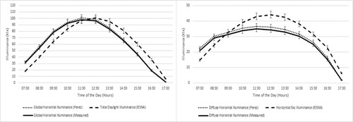
It can be inferred that the values calculated from Perez model are much closer to the measured values than the values calculated from the IESNA recommended calculation procedure. This may be attributed to the simplistic three condition-based sky classification (clear, partly cloudy and cloudy) part in the IESNA recommended calculation procedure which is perceived as a weakness of this procedure (Kandilli and Ulgen 2008). Kittler, Perez, and Darula (1997) proposed a sky classification method with 15 sky categories based on sky conditions and it was accepted by the CIE as CIE standard general sky (CIE 2003). The IESNA recommended calculation procedure may yield better results if it adopts, in a future modification of its original publication, the CIE standard general sky classification method to classify sky types.

3.4. Estimations from window shading control simulation

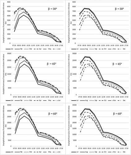
The daylight illuminance transmitted into a room through a window having shading control was calculated in accordance with the methodology proposed by Athienitis and Tzempelikos (2002). External horizontal daylight data obtained from application of Perez model and IESNA recommended calculation procedure were utilised. Calculations were conducted for blind tilt angle (β) values of ${30}^{\circ },{45}^{\circ }\mathrm{and}{60}^{\circ }$ assuming an eastward window with F_w-g = 0.5, F_w-sky = 0.5 and ${\rho }_{\mathrm{g}}=0.2$. Equation (26) was utilised to simplify the glazing transmittance calculations as Equation (27) can only be applied when there is incidence of direct sunlight upon window glazing and windows facing a particular direction receive direct sunlight for a fraction of sunshine duration only. Figure 5 demonstrates the estimated daylight illuminance transmitted into a room through an eastward window with motorised shading control for data obtained from Perez model and Figure 6 demonstrates the same for data obtained from IESNA recommended calculation procedure. For β = ${30}^{\circ }$, the highest and lowest monthly average daylight illuminance transmission through an eastward window with motorised shading control were 4055 lx (July) and 2679 lx (December) respectively for Perez model, and 4098 lx (July) and 2691 lx (December) respectively for IESNA recommended calculation procedure. For β = ${45}^{\circ }$, the highest and lowest monthly average daylight illuminance transmission through an eastward window with motorised shading control were 14730 lx (July) and 9732 lx (December), respectively, for Perez model, and 14,888 lx (July) and 9776 lx (December), respectively, for IESNA recommended calculation procedure. For β = ${60}^{\circ }$, the highest and lowest monthly average daylight illuminance transmission through an eastward window with motorised shading control were 16,913 lx (July) and 11,175 lx (December) respectively for Perez model, and 17,094 lx (July) and 11,224 lx (December), respectively, for IESNA recommended calculation procedure.

Figure 5. Estimation of daylight illuminance transmission into a room through an eastward window with motorised shading control with data obtained from Perez model.

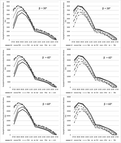
Figure 6. Estimation of daylight illuminance transmission into a room through an eastward window with motorised shading control with data obtained from IESNA recommended calculation procedure.

3.5. Estimations from light pipe simulation

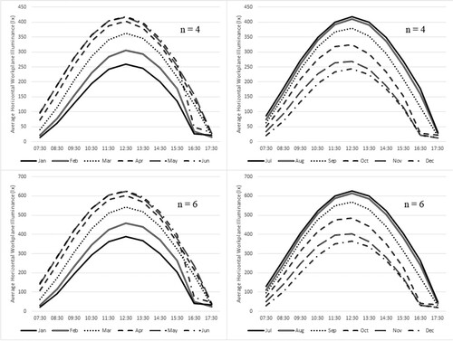
Indoor average horizontal workplane illuminance levels were computed using the methodology as deliberated by Mandal and Roy (2009). Calculations were conducted with Equation (34) for four light pipes (n=4) and six light pipes (n = 6) respectively assuming $A_{\mathrm{d}}$ = 0.2, ${\eta }_{\mathrm{t}}$ = 0.75, $\mathrm{UF}$ = 0.8, $\mathrm{LLF}$ = 0.5 and A = 60. Figure 7 demonstrates the estimated average horizontal workplane illuminance levels for data obtained from Perez model and Figure 8 demonstrates the same for data obtained from IESNA recommended calculation procedure. For four light pipes (n = 4), the highest and lowest monthly average horizontal workplane illuminance levels were 248 lx (April) and 139 lx (December), respectively, for Perez model, and 266 lx (July) and 131 lx (December), respectively, for IESNA recommended calculation procedure. For six light pipes (n = 6), the highest and lowest monthly average horizontal workplane illuminance levels were 371 lx (April) and 209 lx (December), respectively, for Perez model, and 400 lx (July) and 196 lx (December), respectively, for IESNA recommended calculation procedure.

Figure 7. Estimation of average horizontal workplane illuminance from light pipe simulation with data obtained from Perez model.

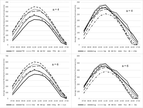
Figure 8. Estimation of average horizontal workplane illuminance from light pipe simulation with data obtained from IESNA recommended calculation procedure.

3.6. Estimations from skylight simulation

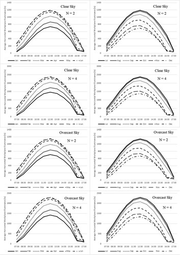
Equations (35) and (36) were used, in accordance with the procedure propounded by Murdoch (1994), to calculate indoor average horizontal workplane illuminance levels for overcast sky and clear sky, respectively. Calculations were conducted for two skylights (N = 2) and four skylights (N = 4) respectively assuming A_s = 0.8, K_usky = 0.75, K_usun = 0.8, K_m = 0.55, K_diffuse = 0.75 and A = 60 m².

Figure 9 demonstrates the estimated average horizontal workplane illuminance levels for data obtained from Perez model and Figure 10 demonstrates the same for data obtained from IESNA recommended calculation procedure. For two skylights (N = 2) with clear sky, the highest and lowest monthly average horizontal workplane illuminance levels were 706 lx (April) and 395 lx (December), respectively, for Perez model, and 757 lx (July) and 369 lx (December), respectively, for IESNA recommended calculation procedure. For two skylights (N = 2) with overcast sky, the highest and lowest monthly average horizontal workplane illuminance levels were 681 lx (April) and 383 lx (December), respectively, for Perez model, and 732 lx (July) and 360 lx (December), respectively, for IESNA recommended calculation procedure. For four skylights (N = 4) with clear sky, the highest and lowest monthly average horizontal workplane illuminance levels were 1412 lx (April) and 789 lx (December), respectively, for Perez model, and 1515 lx (July) and 739 lx (December), respectively, for IESNA recommended calculation procedure. For four skylights (N = 4) with overcast sky, the highest and lowest monthly average horizontal workplane illuminance levels were 1362 lx (April) and 766 lx (December), respectively, for Perez model, and 1465 lx (July) and 719 lx (December), respectively, for IESNA recommended calculation procedure.

Figure 9. Estimation of average horizontal workplane illuminance from skylight simulation with data obtained from Perez model.

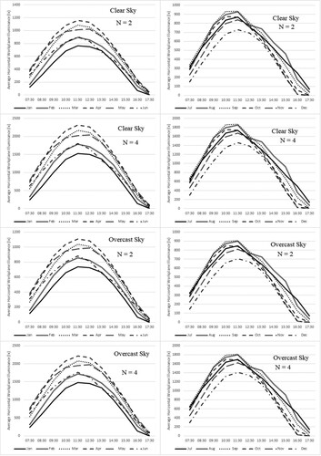
Figure 10. Estimation of average horizontal workplane illuminance from skylight simulation with data obtained from IESNA recommended calculation procedure.

3.7. Estimations from light shelf simulation

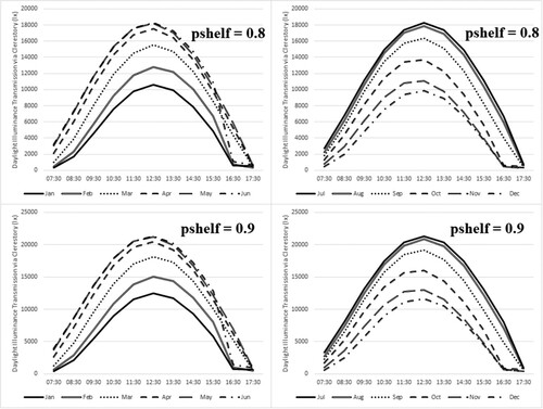
The methodology deliberated by Tsangrassoulis et al. (2019) was utilised to introduce a system of equations (Equations (37–39)) in analogous of photometric quantities which could be used to calculate the daylight transmitted into a room through a clerestory (upper window) due to an externally placed horizontal light shelf. Calculations were conducted for ρ_shelf = 0.8 and 0.9 respectively assuming A_reflected = 0.8 m², F_w-shelf = 0.50, F_sky-shelf = 0.30, A_uw = 2 m² and τ_ν = 0.75.

Figure 11 demonstrates the estimated daylight illuminance transmitted into a room for data obtained from Perez model and Figure 12 demonstrates the same for data obtained from IESNA recommended calculation procedure. For light shelf reflectance of 0.8 (ρ_shelf = 0.8), the highest and lowest monthly average daylight illuminance transmission through a clerestory (upper window) were 10,713 lx (April) and 5531 lx (December), respectively, for Perez model, and 11,106 lx (July) and 4919 lx (December), respectively, for IESNA recommended calculation procedure. For light shelf reflectance of 0.9 (ρ_shelf = 0.9), the highest and lowest monthly average daylight illuminance transmission through a clerestory (upper window) were 12,052 lx (April) and 6223 lx (December), respectively, for Perez model, and 13,043 lx (July) and 5863 lx (December), respectively, for IESNA recommended calculation procedure.

Figure 11. Estimation of daylight illuminance transmission into a room through a clerestory from light shelf simulation with data obtained from Perez model.

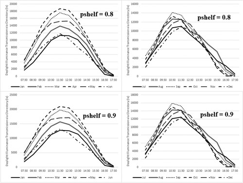
Figure 12. Estimation of daylight illuminance transmission into a room through a clerestory from light shelf simulation with data obtained from IESNA recommended calculation procedure.

4. Discussion

4.1. Percentage cumulative frequency distribution of solar illuminance and luminous efficacy parameters

Figures 13 and 14 provide the percentage cumulative frequency distribution curves of global and diffuse horizontal illuminance for applied Perez model, and total daylight illuminance and horizontal sky (diffuse) illuminance for applied IESNA recommended calculation procedure respectively.

Figure 13. Percentage cumulative frequency curves of global and diffuse horizontal illuminance for applied Perez model.

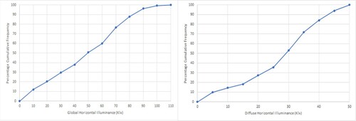
Figure 14. Percentage cumulative frequency curves of total daylight illuminance and horizontal sky illuminance for applied IESNA recommended calculation procedure.

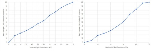
From Figure 13, it can be seen that around 87.88% of the values of global horizontal illuminance are over 10 klx and for diffuse horizontal illuminance it is nearly 85.61%. From Figure 14, in a similar observation, it is seen that around 84.10% of the total daylight illuminance values are over 10 klx and for horizontal sky (diffuse) illuminance it is about 83.34%.

A room is naturally well-lit if the daylight factor (DF) of it is generally over 5%. Assuming a DF of 5%, the extensive availability of external horizontal illuminance levels of 10 klx or more would mean that an indoor illuminance level of 500 lx can ideally be obtained solely from daylighting. Though this simplistic assumption may not always provide accurate estimations and the internally reflected component, which can be calculated by computational algorithms such as the Monte Carlo method (Roy and Bandyopadhya 2002), can widely fluctuate due to the temporally variant nature of daylight. In addition, the mean room surface exitance (MRSE) levels of a daylit indoor space can be estimated by applying experimental procedures (Cuttle 2010; Duff, Antonutto, and Torres 2016; Duff, Kelly, and Cuttle 2017; Cuttle 2018). The information about the daytime MRSE levels can be utilised to estimate the perceived adequacy of illumination (PAI) and target-to-ambient illumination ratio (TAIR) levels for different hours of a day, and it remains an area of significant current research interest.

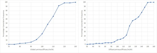
Figure 15 provides the percentage cumulative frequency distribution curves of global and diffuse luminous efficacy for applied Perez model. From Figure 15, it is seen that the global luminous efficacy is higher than 95 lm/W for around 88.64% of all recorded values and around 87.12% of the values lie between 95 and 120 lm/W. Similarly, it is seen that the diffuse luminous efficacy is higher than 110 lm/W for around 84.85% of all recorded values and 84.09% of the values lie between 110 and 150 lm/W.

Figure 15. Percentage cumulative frequency curves of global and diffuse luminous efficacy for applied Perez model.

4.2. Correlation between solar irradiation and solar illuminance

Figure 16 shows the GHI vs. global horizontal illuminance and DHI vs. diffuse horizontal illuminance scatterplots for the applied Perez model. Pearson correlation coefficient test was utilised to measure the strength of linear correlation between irradiation and illuminance. The coefficient of determination (R²) was found to be 0.9866 for the GHI vs. global horizontal illuminance plot, and 0.9234 for the DHI vs. diffuse horizontal illuminance plot. This implies that there is a large positive linear association between irradiation and illuminance in the applied Perez model.

Figure 16. Plots of GHI vs. global horizontal illuminance and DHI vs. diffuse horizontal illuminance for the applied Perez model.

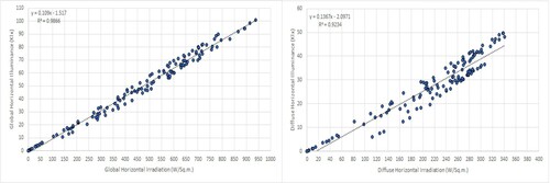
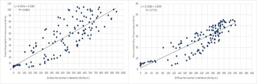
Figure 17 shows the GHI vs. total daylight illuminance and DHI vs. horizontal sky illuminance scatterplots for the applied IESNA recommended calculation procedure. Pearson correlation coefficient test was once again utilised. The coefficient of determination (R²) was 0.6841 for the GHI vs. total daylight illuminance plot, and 0.7751 for the DHI vs. horizontal sky illuminance plot. This implies that the positive linear association between irradiation and illuminance in the applied IESNA recommended calculation procedure is not as strong as that of the applied Perez model and application of Perez model to Kolkata yielded a better coefficient of determination (R²) values.

Figure 17. Plots of GHI vs. total daylight illuminance and DHI vs. horizontal sky illuminance for the applied IESNA recommended calculation procedure.

4.3. Statistical analysis of estimated indoor illuminance levels

The data obtained from global and diffuse horizontal illuminance measurements carried out in April 2020 in Kolkata, India were further utilised to estimate indoor illuminance levels for various daylighting methods, in addition to the estimations obtained from the application of the Perez model and the IESNA recommended calculation procedure for the same period. Table 12 provides a compendium of the statistical analysis carried out with April 2020 data using two statistical indicators: root mean square error (RMSE) and mean absolute error (MAE).

Table 12. Statistical Errors in the Estimation of Indoor Daylight Illuminance Levels.

Daylighting method/device	Matched-pair variables	RMSE	%RMSE	MAE	%MAE
Window shading control	Estimated daylight illuminance transmission from measurement data – estimated daylight illuminance transmission from application of Perez Model	279.82	2.01	266.51	1.91
	Estimated daylight illuminance transmission from measurement data – estimated daylight illuminance transmission from application of IESNA recommended calculation procedure	379.61	9.91	352.06	9.19
Light Pipe	Estimated average horizontal workplane illuminance from measurement data – estimated average horizontal workplane illuminance from application of Perez Model	6.86	2.84	6.18	2.56
	Estimated average horizontal workplane illuminance from measurement data – estimated average horizontal workplane illuminance from application of IESNA recommended calculation procedure	48.85	20.23	44.14	18.28
Skylight (Overcast Sky Condition)	Estimated average horizontal workplane illuminance from measurement data – estimated average horizontal workplane illuminance from application of Perez model	37.74	2.84	33.98	2.56
	Estimated average horizontal workplane illuminance from measurement data – estimated average horizontal workplane illuminance from application of IESNA recommended calculation procedure	268.68	20.23	242.75	18.28
Skylight (Clear Sky Condition)	Estimated average horizontal workplane illuminance from measurement data – estimated average horizontal workplane illuminance from application of Perez model	38.27	2.78	34.24	2.48
	Estimated average horizontal workplane illuminance from measurement data – estimated average horizontal workplane illuminance from application of IESNA recommended calculation procedure	280.13	20.33	253.36	18.39
Light Shelf	Estimated daylight illuminance transmission from measurement data – estimated daylight illuminance transmission from application of Perez model	218.72	2.07	172.01	1.63
	Estimated daylight illuminance transmission from measurement data – estimated daylight illuminance transmission from application of IESNA recommended calculation procedure	2392.71	22.68	2172.13	20.59

5. Conclusion

This work applied two computational methods of predicting solar illuminance, the Perez model and the IESNA recommended calculation procedure, to Kolkata to estimate solar illuminance levels on a horizontal exterior plane, compared the simulated values with those obtained from conducted measurements and calculated approximate daylight illuminance levels for four daylighting devices, namely, motorised shading of windows, light pipes, skylights and light shelves. The statistical analysis in Table 12 demonstrates that the indoor daylight level estimations arrived at from the application of Perez model for various daylighting devices yield acceptable RMSE and MAE. The results clearly indicate that the Perez model could be taken as the better choice in predicting global and diffuse horizontal solar illuminance levels and should be preferred to the IESNA recommended calculation procedure. In addition, the Perez model could be used to estimate global and diffuse luminous efficacy values and the application of this model to Kolkata yielded coefficient of determination (R²) values over 0.92, indicating a large positive linear association between irradiation and illuminance. From the applied Perez model to Kolkata, the estimated yearly average global and diffuse luminous efficacy values are 105.00 and 123.92 lm/W, respectively, and the estimated yearly average global horizontal and diffuse horizontal illuminance values are 47.71 and 27.00 klx, respectively. This is an indicator of the promising daylighting potential of Kolkata which should be harnessed by architects, construction engineers, building services engineers and interior designers.

This work may serve as a paradigm in estimating the indoor daylight availability from solar radiation databases in energy-efficient building planning for different geographical locations. Daylighting can reduce electrical energy expenditure in artificial illumination (Mistrick and Sarkar 2005; Ihm, Nemri, and Krarti 2009), improve visual comfort and mood (Borisuit et al. 2015; Shishegar and Boubekri 2016; Asojo, Bae, and Martin 2020), increase employee productivity (Thayer 1995) and lighting controls responsive to daylight, such as dimmable electronic ballasts (Doulos, Tsangrassoulis, and Topalis 2008) can extensively save energy and cut down the financial incurrences. Daylight influx can be controlled and redistributed in indoor spaces through the use of light shelves (Beltran, Lee, and Selkowitz 1997; Lim and Heng 2016), light pipes and skylights (Beltran et al. 1994). In addition, shading devices, such as roller shades, prismatic louvres and venetian blinds, can be utilised to selectively admit daylight and control glare (Nilsson and Jonsson 2010; Eltaweel et al. 2020), often in tandem with daylight responsive artificial lighting controls. Currently, LEDs are viewed as a viable source for general indoor illumination due to the light output, luminous efficacy and minimal colour shift (Protzman and Houser 2006) and recent works have explored energy-saving aspects of daylight integration with LED-based indoor illumination systems (Ge et al. 2014; Doulos et al. 2017). Integration of daylighting systems to already installed artificial indoor illumination systems is of sustained interest to researchers worldwide and combining it with renewable energy sources can conserve energy, reduce carbon emission, increase human productivity in offices, schools and other institutions, and provide far-reaching benefits to public health, morale and wellbeing.

Acknowledgements

The authors duly credit and express gratitude to the U.S. Department of Energy (DOE)/National Renewable Energy Laboratory (NREL)/Alliance for Sustainable Energy LLC (ALLIANCE) for providing the 2014 SUNY semi-empirical model solar irradiance data of Kolkata, India from the National Solar Radiation Database (NSRDB), maintained by the National Renewable Energy Laboratory (NREL), via e-mail to the corresponding author upon request. The information reproduced in this work from the PVGIS-5 geo-temporal irradiation database is authorised by the PVGIS, European Union, as the source of information is duly cited in the text. The authors would also like to express gratefulness to the anonymous referees for offering their expertise to constructively review the paper which assisted the authors to enhance the quality of the paper.

Disclosure statement

No potential conflict of interest was reported by the author(s).

References

- Al-Ashwal, N. T., and A. S. Hassan. 2017. “Estimation of Energy Savings Due to the Integration of Daylight with Artificial Lighting in Classrooms.” Advanced Science Letters 23 (7): 6140–6143.
- Alrubaih, M. S., M. F. M. Zain, M. A. Alghoul, N. L. N. Ibrahim, M. A. Shameri, and O. Elayeb. 2013. “Research and Development on Aspects of Daylighting Fundamentals.” Renewable and Sustainable Energy Reviews 21: 494–505.
- Asojo, A. O., S. Bae, and C. S. Martin. 2020. “Post-occupancy Evaluation Study of the Impact of Daylighting and Electric Lighting in the Workplace.” Leukos 16 (3): 239–250.
- Athienitis, A. K., and A. Tzempelikos. 2002. “A Methodology for Simulation of Daylight Room Illuminance Distribution and Light Dimming for a Room with a Controlled Shading Device.” Solar Energy 72 (4): 271–281.
- Azad, A. S., D. Rakshit, and K. N. Patil. 2018. “Model Development and Evaluation of Global and Diffuse Luminous Efficacy for Humid Sub-Tropical Region.” Renewable Energy 119: 375–387.
- Bahdad, A. A. S., S. F. S. Fadzil, and N. Taib. 2020. “Optimization of Daylight Performance Based on Controllable Light-Shelf Parameters Using Genetic Algorithms in the Tropical Climate of Malaysia.” Journal of Daylighting 7 (1): 122–136.
- Bellia, L., and F. Fragliasso. 2017. “New Parameters to Evaluate the Capability of a Daylight-Linked Control System in Complementing Daylight.” Building and Environment 123: 223–242.
- Beltran, L. O., E. S. Lee, K. M. Papmichael, and S. E. Selkowitz. 1994. The Design and Evaluation of Three Advanced Daylighting Systems: Light Shelves, Light Pipes and Skylights (No. LBL-34458; CONF-9406134-4). Berkeley, CA: Lawrence Berkeley Lab.
- Beltran, L. O., E. S. Lee, and S. E. Selkowitz. 1997. “Advanced Optical Daylighting Systems: Light Shelves and Light Pipes.” Journal of the Illuminating Engineering Society 26 (2): 91–106.
- Binarti, F., and S. Dewi. 2016. “The Effectiveness of Light Shelf in Tropical Urban Context.” Environmental and Climate Technologies 18 (1): 42–53.
- Bisegna, F., C. Burattini, M. Manganelli, L. Martirano, B. Mattoni, and L. Parise. 2016, June. “Adaptive Control for Lighting, Shading and HVAC Systems in Near Zero Energy Buildings.” 2016 IEEE 16th International Conference on Environment and Electrical Engineering (EEEIC), IEEE, 1–6.
- Borisuit, A., F. Linhart, J. L. Scartezzini, and M. Münch. 2015. “Effects of Realistic Office Daylighting and Electric Lighting Conditions on Visual Comfort, Alertness and Mood.” Lighting Research & Technology 47 (2): 192–209.
- Canazei, M., M. Laner, S. Staggl, W. Pohl, P. Ragazzi, D. Magatti, E. Martinelli, and P. Di Trapani. 2016. “Room- and Illumination-Related Effects of an Artificial Skylight.” Lighting Research & Technology 48 (5): 539–558.
- Canazei, M., W. Pohl, H. R. Bliem, M. Martini, and E. M. Weiss. 2017. “Artificial Skylight Effects in a Windowless Office Environment.” Building and Environment 124: 69–77.
- Carter, D. J. 2002. “The Measured and Predicted Performance of Passive Solar Light Pipe Systems.” Lighting Research & Technology 34 (1): 39–51.
- Chaiwiwatworakul, P., and S. Chirarattananon. 2013. “Luminous Efficacies of Global and Diffuse Horizontal Irradiances in a Tropical Region.” Renewable Energy 53: 148–158.
- Chakrabarti, S., and S. Chakrabarti. 2002. “Rural Electrification Programme with Solar Energy in Remote Region – A Case Study in an Island.” Energy Policy 30 (1): 33–42.
- Chakraborty, S., P. Barua, S. Bhattacharjee, and S. Mazumdar. 2018. “Road Classification Based Energy Efficient Design and its Validation for Indian Roads.” Light & Engineering 26 (2): 110–121.
- CIE. 2003. Spatial Distribution of Daylight – CIE Standard General Sky. Standard CIE S 011/E:2003.
- Colaco, S. G., C. P. Kurian, V. I. George, and A. M. Colaco. 2008. “Prospective Techniques of Effective Daylight Harvesting in Commercial Buildings by Employing Window Glazing, Dynamic Shading Devices and Dimming Control – A Literature Review.” Building Simulation 1 (1): 279–289.
- Cuttle, C. 1983, June. “People and Windows in Workplaces.” Proceedings of the People and Physical Environment Research Conference, Wellington, New Zealand, 203–212.
- Cuttle, C. 2010. “Towards the Third Stage of the Lighting Profession.” Lighting Research & Technology 42 (1): 73–93.
- Cuttle, C. 2018. “A Fresh Approach to Interior Lighting Design: The Design Objective – Direct Flux Procedure.” Lighting Research & Technology 50 (8): 1142–1163.
- D'Agostino, D., and D. Parker. 2018. “A Framework for the Cost-Optimal Design of Nearly Zero Energy Buildings (NZEBs) in Representative Climates Across Europe.” Energy 149: 814–829.
- Dalla Costa, M. A., L. Schuch, L. Michels, C. Rech, J. R. Pinheiro, and G. H. Costa. 2010. “Autonomous Street Lighting System Based on Solar Energy and LEDs.” 2010 IEEE International Conference on Industrial Technology, Via del Mar, Chile. IEEE, 1143–1148.
- Darula, S. 2018. “Review of the Current State and Future Development in Standardizing Natural Lighting in Interiors.” Light & Engineering 26 (4): 5–26.
- Deroisy, B., and A. Deneyer. 2017. “A New Standard for Daylight: Towards a Daylight Revolution.” Proc. International Conference on Lux Europa 2017, LES Slovenia: 340–343.
- Dieste-Velasco, M. I., M. Díez-Mediavilla, D. Granados-López, D. González-Peña, and C. Alonso-Tristán. 2019. “Performance of Global Luminous Efficacy Models and Proposal of a New Model for Daylighting in Burgos, Spain.” Renewable Energy 133: 1000–1010.
- Doulos, L. T., A. Kontadakis, E. N. Madias, M. Sinou, and A. Tsangrassoulis. 2019. “Minimizing Energy Consumption for Artificial Lighting in a Typical Classroom of a Hellenic Public School Aiming for Near Zero Energy Building Using LED DC Luminaires and Daylight Harvesting Systems.” Energy and Buildings 194: 201–217.
- Doulos, L. T., A. Tsangrassoulis, P. A. Kontaxis, A. Kontadakis, and F. V. Topalis. 2017. “Harvesting Daylight with LED or T5 Fluorescent Lamps? The Role of Dimming.” Energy and Buildings 140: 336–347.
- Doulos, L., A. Tsangrassoulis, and F. Topalis. 2008. “Quantifying Energy Savings in Daylight Responsive Systems: The Role of Dimming Electronic Ballasts.” Energy and Buildings 40 (1): 36–50.
- Duff, J., G. Antonutto, and S. Torres. 2016. “On the Calculation and Measurement of Mean Room Surface Exitance.” Lighting Research & Technology 48 (3): 384–388.
- Duff, J., K. Kelly, and C. Cuttle. 2017. “Spatial Brightness, Horizontal Illuminance and Mean Room Surface Exitance in a Lighting Booth.” Lighting Research & Technology 49 (1): 5–15.
- Duffy, J. F., and K. P. Wright. 2005. “Entrainment of the Human Circadian System by Light.” Journal of Biological Rhythms 20 (4): 326–338.
- Eltaweel, A., M. A. Mandour, Q. Lv, and Y. Su. 2020. “Daylight Distribution Improvement Using Automated Prismatic Louvre.” Journal of Daylighting 7 (1): 84–92.
- Fasi, M. A., and I. M. Budaiwi. 2015. “Energy Performance of Windows in Office Buildings Considering Daylight Integration and Visual Comfort in hot Climates.” Energy and Buildings 108: 307–316.
- Ferenčíková, M., and S. Darula. 2017. “Availability of Daylighting in School Operating Time.” Light & Engineering 25 (2): 71–78.
- Galasiu, A. D., and J. A. Veitch. 2006. “Occupant Preferences and Satisfaction with the Luminous Environment and Control Systems in Daylit Offices: A Literature Review.” Energy and Buildings 38 (7): 728–742.
- Ge, A., P. Qiu, J. Cai, W. Wang, and J. Wang. 2014. “Hybrid Daylight/Light-Emitting Diode Illumination System for Indoor Lighting.” Applied Optics 53 (9): 1869–1873.
- Ghisi, E., and J. A. Tinker. 2005. “An Ideal Window Area Concept for Energy Efficient Integration of Daylight and Artificial Light in Buildings.” Building and Environment 40 (1): 51–61.
- Heerwagen, J. H., and D. R. Heerwagen. 1986. “Lighting and Psychological Comfort.” Lighting Design and Application 16 (4): 47–51.
- Henderson, S. T., and D. Hodgkiss. 1963. “The Spectral Energy Distribution of Daylight.” British Journal of Applied Physics 14 (3): 125–131.
- IES Calculation Procedures Committee. 1984. “Recommended Practice for the Calculation of Daylight Availability.” Journal of the Illuminating Engineering Society 13 (4): 381–392.
- Ihm, P., A. Nemri, and M. Krarti. 2009. “Estimation of Lighting Energy Savings from Daylighting.” Building and Environment 44 (3): 509–514.
- Joshi, M., R. L. Sawhney, and D. Buddhi. 2007. “Estimation of Luminous Efficacy of Daylight and Exterior Illuminance for Composite Climate of Indore City in Mid Western India.” Renewable Energy 32 (8): 1363–1378.
- Kabir, E., P. Kumar, S. Kumar, A. A. Adelodun, and K. H. Kim. 2018. “Solar Energy: Potential and Future Prospects.” Renewable and Sustainable Energy Reviews 82: 894–900.
- Kalogirou, S. A. 2004. “Environmental Benefits of Domestic Solar Energy Systems.” Energy Conversion and Management 45 (18–19): 3075–3092.
- Kalogirou, S. A. 2014. “Chapter 2-Environmental Characteristics.” Solar Energy Engineering, 92–95. doi:https://doi.org/10.1016/B978-0-12-397270-5.01001-3.
- Kandilli, C., and K. Ulgen. 2008. “Solar Illumination and Estimating Daylight Availability of Global Solar Irradiance.” Energy Sources, Part A: Recovery, Utilization, and Environmental Effects 30 (12): 1127–1140.
- Karakoti, I., P. K. Das, and S. K. Singh. 2012. “Predicting Monthly Mean Daily Diffuse Radiation for India.” Applied Energy 91 (1): 412–425.
- Kasten, F. 1993. “Discussion on the Relative Optical air Mass.” Lighting Research and Technology 25 (3): 129–130.
- Kaufman, J. E. 1981. IES Lighting Handbook: 1981 Application Volume (Vol. 2). New York: Illuminating Engineering Society of North America.
- Kittler, R., R. Perez, and S. Darula. 1997. “A New Generation of Sky Standards.” Proceedings of the Lux Europa 97: 359–373.
- Knoop, M., O. Stefani, B. Bueno, B. Matusiak, R. Hobday, A. Wirz-Justice, K. Martiny, et al. 2020. “Daylight: What Makes the Difference?” Lighting Research & Technology 52 (3): 423–442.
- Konstantoglou, M., and A. Tsangrassoulis. 2016. “Dynamic Operation of Daylighting and Shading Systems: A Literature Review.” Renewable and Sustainable Energy Reviews 60: 268–283.
- Kontadakis, A., A. Tsangrassoulis, L. Doulos, and S. Zerefos. 2018. “A Review of Light Shelf Designs for Daylit Environments.” Sustainability 10 (1): 01–24.
- Kose, B., and T. Kazanasmaz. 2020. “Applicability of a Prismatic Panel to Optimize Window Size and Depth of a South-Facing Room for a Better Daylight Performance.” Light & Engineering 28 (4): 63–67.
- Kousalyadevi, G., and G. Lavanya. 2019. “Optimal Investigation of Daylighting and Energy Efficiency in Industrial Building Using Energy-Efficient Velux Daylighting Simulation.” Journal of Asian Architecture and Building Engineering 18 (4): 271–284.
- Lam, Y. M., and J. H. Xin. 2002. “Evaluation of the Quality of Different D65 Simulators for Visual Assessment.” Color Research & Application 27 (4): 243–251.
- Lee, H., K. Kim, J. Seo, and Y. Kim. 2017. “Effectiveness of a Perforated Light Shelf for Energy Saving.” Energy and Buildings 144: 144–151.
- Lim, Y. W., and C. Y. S. Heng. 2016. “Dynamic Internal Light Shelf for Tropical Daylighting in High-Rise Office Buildings.” Building and Environment 106: 155–166.
- Littlefair, P. J. 1985. “The Luminous Efficacy of Daylight: A Review.” Lighting Research & Technology 17 (4): 162–182.
- Littlefair, P. J. 1995. “Light Shelves: Computer Assessment of Daylighting Performance.” Lighting Research and Technology 27 (2): 79–91.
- Mandal, P., and B. Roy. 2016, December. “Adaptive Dimming Scheme Based Daylight Pipe Integrated Indoor Lighting System Under Perez All-Weather sky Model.” 2016 IEEE International WIE Conference on electrical and computer Engineering (WIECON-ECE), IEEE: 221–224.
- Maňková, L., J. Hraška, and M. Janak. 2009. “Simplified Determination of Indoor Daylight Illumination by Light Pipes.” Slovak Journal of Civil Engineering 4: 22–30.
- Markus, T. A. 1967. “The Function of Windows— A Reappraisal.” Building Science 2 (2): 97–121.
- Mistrick, R., and A. Sarkar. 2005. “A Study of Daylight-Responsive Photosensor Control in Five Daylighted Classrooms.” LEUKOS The Journal of the Illuminating Engineering Society of North America 01 (3): 51–74.
- Molina, L. J., R. I. Maestre, and E. Lindawer. 2000. “A Model for Predicting the Angular Dependence of the Optical Properties of Complex Windows Including Shading Devices.” Proceedings of PLEA, Cambridge, 765–770.
- Muneer, T. 1996. “Evaluation of Luminous Efficacy Models Against Japanese Data: Technical Note.” International Journal of Ambient Energy 17 (4): 212–216.
- Muneer, T., and R. C. Angus. 1993. “Daylight Illuminance Models for the United Kingdom.” Lighting Research and Technology 25 (3): 113–123.
- Murdoch, J. B. 1994. Illumination Engineering: From Edison's Lamp to the Laser. New York: Macmillan Publishing Company.
- Nilsson, A. M., and J. C. Jonsson. 2010. “Light-scattering Properties of a Venetian Blind Slat Used for Daylighting Applications.” Solar Energy 84 (12): 2103–2111.
- NREL. 2014. International Data. Accessed May 20, 2020. https://nsrdb.nrel.gov/about/international-data.html.
- Okogbue, E. C., J. A. Adedokun, and B. Holmgren. 2008. “Hourly and Daily Global Photometric Illuminance and Luminous Efficacy at a Tropical Station, Ile-Ife, Nigeria.” International Journal of Sustainable Energy 27 (3): 105–120.
- Patil, K. N., S. N. Garg, and S. C. Kaushik. 2013. “Luminous Efficacy Model Validation and Computation of Solar Illuminance for Different Climates of India.” Journal of Renewable and Sustainable Energy 5 (6): 063120.
- Perez, R., P. Ineichen, R. Seals, J. Michalsky, and R. Stewart. 1990. “Modeling Daylight Availability and Irradiance Components from Direct and Global Irradiance.” Solar Energy 44 (5): 271–289.
- Pikas, E., M. Thalfeldt, and J. Kurnitski. 2014. “Cost Optimal and Nearly Zero Energy Building Solutions for Office Buildings.” Energy and Buildings 74: 30–42.
- Powell, I. 1996. “D65 Simulation with a Xenon Arc.” Applied Optics 35 (34): 6708–6713.
- Protzman, J. B., and K. W. Houser. 2006. “LEDS for General Illumination: The State of the Science.” Leukos 3 (2): 121–142.
- PVGIS. 2020. PVGIS-5 Geo-Temporal Irradiation Database. Accessed May 20, 2020. https://ec.europa.eu/jrc/en/pvgis.
- Rao, K. R., and T. N. Seshadri. 1961. “Solar Insolation Curves.” Indian Journal of Meteorology and Geophysics 12: 267–272.
- Raul, D., S. Pal, and B. Roy. 2015. “Application of Perez Daylight Efficacy Model for Kolkata.” Journal of The Institution of Engineers (India): Series B 96 (4): 339–348.
- Roenneberg, T., T. Kantermann, M. Juda, C. Vetter, and K. V. Allebrandt. 2013. “Light and the Human Circadian Clock.” In Circadian Clocks. Handbook of Experimental Pharmacology. Vol. 217, edited by A. Kramer and M. Merrow, 311–331. Berlin: Springer. doi:https://doi.org/10.1007/978-3-642-25950-0_13.
- Roy, B., and S. R. Bandyopadhya. 2002. “Interreflection Calculation Under Daylight by Monte Carlo Method.” Journal of Optics 31 (3): 95–104.
- Samuhatananon, S., S. Chirarattananon, and P. Chirarattananon. 2011. “An Experimental and Analytical Study of Transmission of Daylight Through Circular Light Pipes.” Leukos 7 (4): 203–219.
- Sengupta, M., Y. Xie, A. Lopez, A. Habte, G. Maclaurin, and J. Shelby. 2018. “The National Solar Radiation Data Base (NSRDB).” Renewable and Sustainable Energy Reviews 89: 51–60.
- Shahsavari, A., and M. Akbari. 2018. “Potential of Solar Energy in Developing Countries for Reducing Energy-Related Emissions.” Renewable and Sustainable Energy Reviews 90: 275–291.
- Shin, J. Y., G. Y. Yun, and J. T. Kim. 2012. “Evaluation of Daylighting Effectiveness and Energy Saving Potentials of Light-Pipe Systems in Buildings.” Indoor and Built Environment 21 (1): 129–136.
- Shishegar, N., and M. Boubekri. 2016. “April. Natural Light and Productivity: Analyzing the Impacts of Daylighting on Students’ and Workers’ Health and Alertness.” Proceedings of the International Conference on “health, Biological and life science” (HBLS-16), Istanbul, Turkey, 18–19.
- Soler, A., and P. Oteiza. 1997. “Light Shelf Performance in Madrid, Spain.” Building and Environment 32 (2): 87–93.
- Solovyov, A. K. 2017. “Reflective Facades and Their Influence on Illumination of Nearby Buildings.” Light & Engineering 25 (2): 88–93.
- Thayer, B. M. 1995. “Daylighting and Productivity at Lockheed.” Solar Today 9 (3): 26–29.
- Tsangrassoulis, A., L. Doulos, A. Kontadakis, and A. Drakou. 2019. “A Methodology to Model the Performance of a Dynamic Mirror Light-Shelf Based on Solar Radiant Flux Impinging on the Window.” Proceedings of the 16th IBPSA Conference, International Building Performance Simulation Association, Rome, Italy, 1028–1035. doi:https://doi.org/10.26868/25222708.2019.210483.
- Turan, I., A. Chegut, D. Fink, and C. Reinhart. 2020. “The Value of Daylight in Office Spaces.” Building and Environment 168: 106503.
- Van Derlofske, J. F., and T. A. Hough. 2004. “Analytical Model of Flux Propagation in Light-Pipe Systems.” Optical Engineering 43 (7): 1503–1511.
- Wang, J., and Y. Yang. 2016. “Energy, Exergy and Environmental Analysis of a Hybrid Combined Cooling Heating and Power System Utilizing Biomass and Solar Energy.” Energy Conversion and Management 124: 566–577.
- Woelders, T., D. G. Beersma, M. C. Gordijn, R. A. Hut, and E. J. Wams. 2017. “Daily Light Exposure Patterns Reveal Phase and Period of the Human Circadian Clock.” Journal of Biological Rhythms 32 (3): 274–286.
- Wright, J., R. Perez, and J. J. Michalsky. 1989. “Luminous Efficacy of Direct Irradiance: Variations with Insolation and Moisture Conditions.” Solar Energy 42 (5): 387–394.
- Xue, P., C. M. Mak, and H. D. Cheung. 2014. “The Effects of Daylighting and Human Behavior on Luminous Comfort in Residential Buildings: A Questionnaire Survey.” Building and Environment 81: 51–59.
- Yao, J. 2018. “Daylighting Performance of Manual Solar Shades.” Light & Engineering 26 (1): 99–104.
- Yasukouchi, A., T. Maeda, K. Hara, and H. Furuune. 2019. “Non-visual Effects of Diurnal Exposure to an Artificial Skylight, Including Nocturnal Melatonin Suppression.” Journal of Physiological Anthropology 38 (1): 1–12.
- Yun, G. Y., T. Hwang, and J. T. Kim. 2010. “Performance Prediction by Modelling of a Light-Pipe System Used Under the Climate Conditions of Korea.” Indoor and Built Environment 19 (1): 137–144.
- Zazzini, P., A. Romano, A. Di Lorenzo, V. Portaluri, and A. Di Crescenzo. 2020. “Experimental Analysis of the Performance of Light Shelves in Different Geometrical Configurations Through the Scale Model Approach.” Journal of Daylighting 7 (1): 37–56.