Prediction of the near wall flow behaviours of separation and transition for NREL phase VI wind turbine blade

ABSTRACT

This study demonstrates the separation and transition flow behaviour around a 3-D wind turbine blade by analysing blending functions, intermittency, and transition onset Reynolds number in SST Gamma Theta model. The National Renewable Energy Laboratory Phase VI rotor was modelled for the analysis. The simulations were executed by using the ANSYS-CFX solver. Extensive comparisons were performed to demonstrate the accuracy of this numerical model for sectional pressure distribution, tangent force, normal force, thrust, and torque. Good agreement was observed in all wind speed cases. The discrepancies in pre-stall region were negligible, and those in the post-stall region were acceptable. Thus, the capability and accuracy of the SST Gamma Theta model in predicting separated and transitional flow effects were verified.

KEYWORDS:

• CFD
• SST Gamma Theta
• blending function
• separation
• intermittency
• transition onset Reynolds number

1. Introduction

Wind energy is one of the cleanest, sustainable, and abundant renewable energy resources. Wind turbines are used to harness this wind energy. One of the fundamental technological components in a wind power generation system is the wind turbine blades. Thus, numerous efforts to develop unique blades or optimise existing blade designs have been made by many research institutes.

During the design and development of new, efficient, and reliable wind turbine blades, accurate aerodynamic force predictions and optimised aerodynamic design are necessary because the interaction between the blades and wind significantly influences the efficiency and ultimately affects the lifespan of the wind turbine. Thus, it is essential to know the characteristic results of the flow field and aerodynamic performance. Wind tunnel test is considered to be an accurate and reliable way to investigate wind turbine blades. However, it needs comprehensive knowledge and high-quality equipment to operate the experiment. One of important wind tunnel test data reported by National Renewable Energy Lab (NREL) to the public is NREL Phase VI wind turbine blade reports (Schreck, Hand, and Fingersh 2001; Hand et al. 2001), which used the S809 aerofoil (Ramsay, Hoffmann, and Gregorek 1995) as the blade section, and have been used by many researchers to verify their work.

In addition to wind tunnel tests, various highly complicated numerical approaches have been developed to predict aerodynamic behaviour, including blade element momentum (BEM) theory and computational fluid dynamics (CFD). Wind turbine blades are traditionally designed using BEM theory with lift and drag coefficients defined by two-dimensional (2D) aerofoil data from wind tunnel tests, which means BEM theory is highly dependent on wind tunnel experiments. When applying BEM methods to higher wind speeds to predict rotor power, possible errors can happen which are mainly caused by inadequacies of evaluating accurate 3D aerodynamic force characteristics for the fully separation and stall conditions. Therefore, experimental corrections, including tip losses, root losses, dynamic stall effects, and rotational effects, are often applied to make the predictions as close as possible to the real data. For instance, Dai et al. (2011) studied the aerodynamic characteristics of turbine blades using a dynamic stall model and a modified BEM theory. Lanzafame and Messina (2012) considered the radial flow in BEM theory. Furthermore, based on BEM theory, a code incorporating tip loss was also developed and proved to be reasonably accurate in evaluating the aerodynamic parameters of horizontal axis wind turbines by Sharifi and Nobari (2013).

The CFD is becoming one an important tool in wind turbine research. Many hypothetical models have been developed for turbulent flow simulation. Those that are based on the Reynolds-averaged Navier–Stokes equations (RANS) are the most widely used. Such models provide detailed information and visual representations of airflows in various critical areas, which helps researchers understand the 3D aerodynamics of the rotor which can analyse the complex 3D geometry commonly. However, CFD also has many difficulties, such as requiring more computing time and technical skills to obtain acceptable results. Fortunately, as the computational capacity of computers and the user-friendliness of software are improved, researchers are overcoming these difficulties. Thus, a number of researchers have used CFD to obtain the aerodynamic design of wind turbines. For instance, computations of the NREL Phase VI wind turbine using the RANS flow solver Overflow-D2 were performed by Duque, Burklund, and Johnson (2003). They compared the experimental data with the Overflow-D2 results and found that good agreement was achieved for the power and spanwise loading of the wind turbine. Sezer-Uzol and Long (2006) calculated the blade parameters at various wind speeds and yaw angles and showed acceptable results in comparison with the NREL Phase VI experimental data, except in the massive flow separation situation. Potsdam and Mavriplis (2009) applied RANS code to investigate an isolated wind turbine rotor and found that the results were in good agreement with the experimental data. Lee et al. (2012) evaluated the blunt effects by modifying the original NREL Phase VI blade using the RANS-based turbulent model using Fluent. In addition, large eddy simulation (LES), which overcomes the disadvantages of the steady-state RANS equations, such as the inability to capture unsteadiness resulting from vortex shedding, was performed by Mo et al. (2013) to study the effect of variation in wind speed on transient wake instability. The simulation results were also compared with experimental data and were found to be in good agreement.

Many general-purpose RANS-based turbulent models show an inability to accurately predict the onset of separation behaviour or flow reattachment. However, the shear stress transport (SST) turbulent model achieves an optimal formulation by combining the k–ω and k–ϵ models (Menter 1994; Menter 2009). Mo and Lee (2012) investigated the accuracy of the SST turbulent model and reported a comparison with experimental data to verify the validity of the analysis results. Li et al. (2012) simulated unsteady aerodynamics using detached eddy simulation (DES).

Moshfeghi, Song, and Xie (2012), Lanzafame, Mauro, and Messina (2013), and Yelmule and Vsj (2013) used the SST Gamma theta model to take into account both of separation and transitional flow effect on NREL Phase VI wind turbine using commercial CFD tools. In these researches, the extensive and comprehensive studies were performed to show the accuracy of applied SST Gamma Theta model, and showed good agreement with experiments. Lanzafame, Mauro, and Messina (2013) in his works perform numerical simulation to calculate lift coefficient, power coefficient, Y + effect, etc. to analyse the turbulence model and its efficiency in predicting blade flow outcome. Yelmule and Vsj (2013) in their research considered experimental analysis of wind turbine blade at 7–10 m/s velocity and later validated their numerical simulation using experimental data. Since they considered 10 m/s or below they did not discuss stall effects at higher velocities.

In the boundary layer of fluid flows, separated and transitional flows greatly influence many engineering applications, such as wind turbine blade rotation. Furthermore, the location and characteristics of the onset and the extent of separation and its effect on the transition are important in the design and performance of wind turbine blades. The SST turbulent model commonly overestimates the flow dissipation from the leading edge of the aerofoil. To address the transition effect more accurately Menter et al. developed the Gamma Theta correlation model (2003, 2006a, 2006b). The correlation is combined with SST model the mathematical formulation of which is mentioned in part-I of the paper on (2006a). It is an empirical correlations-based transition model with two transport equations that utilise only local parameters, one for the intermittency and one for the transition onset criteria. It is a very popular transitional model for general-purpose applications. Additionally, several new empirical correlations, which have been developed to cover standard bypass transitions as well as flows in low free-stream turbulent environments, are currently utilised and have been extensively validated by Menter et al in the Part-2 of the publication (2006b) for a wide range of transitional flows. This transitional model contributes to the formation of the SST Gamma Theta model, which builds the turbulent boundary layer from the transition point and produces a more accurate result.

Even though valuable results were described in their research for the accuracies and advantages of SST Gamma Theta model, details of separation and separation-induced transitional flow under low to higher wind speed were not demonstrated sufficiently. The effect on the stall and transition-induced stall has more significance at mid to high wind speed condition (10–25 m/s) which is considered in previous researches. Moreover, to analyse better numerically the prediction of transition effect, blending function is an effective prospective. It helps to clearly explain intermittency and transition onset Reynolds number. In authors knowledge which are not available in any literature. Most studies focused on the accuracy and applicability of this model by comparing the results of the aerodynamic force and pressure coefficient with the NREL experimental data. Thus, in this study, the separation and transition on the NREL Phase VI wind turbine blade using the SST Gamma Theta model were analysed and the sectional pressure coefficient, velocity coefficient contours, sectional aerodynamic force, and streamline results were evaluated. In addition, the results of intermittency and transition onset Reynolds number were clearly explained with the help of the blending functions. The accuracies of these studies were demonstrated by comparison with experimental data. The advantage of using blending function, intermittency, and transition onset Reynolds number in analysing complex flow behaviour at near wall during separation and transition has been identified and discussed through this work which will be a valuable method for future wind turbine blade studies.

2. Specifications of NREL phase VI wind turbine blades

The NREL has conducted complicated experiments on wind turbine performance. To take 3D effects into account and acquire accurate quantitative aerodynamic and structural wind turbine measurements, in May 2000, a successful test of the upwind NREL Phase VI wind turbine was conducted in the NASA Ames wind tunnel (Hand et al. 2001). In December 2001, NREL published a publicly available technical report that included details of the experimental data of the blade (Schreck, Hand, and Fingersh 2001; Hand et al. 2001). Thus, the performances of developed analytical codes were demonstrated by comparing with the reported data.

In this study, the blade shape used in the NREL Phase VI test was adopted for CFD simulation. The NREL Phase VI wind turbine tested in the NASA wind tunnel is stall-regulated and produces a rated output power of 19.8 kW. The turbine blade diameter is D = 10.058 m, the blade number is Z = 2, and the rotational speed is N = 71.9 rpm (N = 72 rpm is adopted in this study).

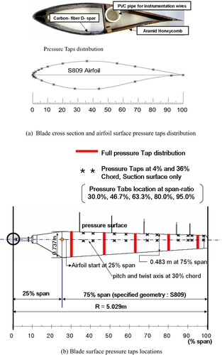
Blade surface pressure measurements play a critical role in the quality of the aerodynamic performance because the aerodynamic coefficients are integrated from the installed measured pressure taps, which were distributed on the surface of the blade skin. Five span-wise locations (r/R = 30.0%, 46.6%, 63.3%, 80.0%, and 95.0% of the span) were selected to be instrumented with the 22 pressure taps on both the suction and pressure surfaces. More taps were located near the leading edge to obtain a more accurate solution in the more active regions of the aerofoil. The geometry and pressure tap distribution of the NREL Phase VI wind turbine blade section is presented in Figure 1(a). Particularly, pairs of taps, located on the 4% and 36% chords, were adopted on the suction surface along the spanwise direction, as shown in Figure 1(b).

Figure 1. NREL Phase VI 2D and 3D pressure distribution. (a) Blade cross section and aerofoil surface pressure taps distribution; (b) Blade surface pressure taps locations.

3. CFD modelling processes

Besides the calculation process, pre-processing and post-processing are also two critical steps in CFD simulation. Pre-processing involves the creation of the geometry model, meshing, and the setup of boundary conditions. And the post-processing is the final step of the CFD analysis. It mainly focuses on the interpretation, analysation, and visualisation of the simulation results. This chapter explains the pre-processing in details.

3.1. Geometry construction

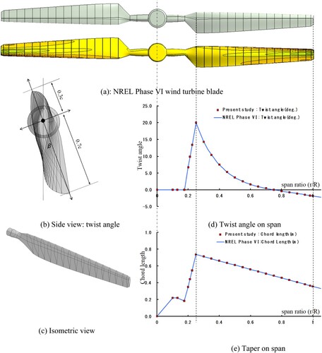
Although the entire wind turbine system was initially tested in a wind tunnel experimental study, the tower and nacelle were ignored to simplify the CFD model. In this study, only the blade was investigated. The actual taper and twist of the blade were considered to resolve the real 3D flow field. The blade design is incorporated from same group previous work (Lee et al. 2016a), as shown in Figure 2. It is built by a series of original sharp-edged S809 aerofoils from root to tip. This well-documented aerofoil is optimised to be less sensitive to leading edge roughness to improve the wind energy output power (Schreck, Hand, and Fingersh 2001; Hand et al. 2001). Along the entire blade, the minimum chord length is 0.356 m, and the maximum chord length is 0.737 m. The twist axis is located at 30.0% to chord length. The maximum twist angle is 20.04°, which occurs at 25% of the span and decreases to a –2.5° twist at the tip. In addition to the aerofoil, a cylinder with a 0.109 m radius that extends from 0.508 m to 0.883 m also exists, and a transitional part was designed to connect the circular section to the root aerofoil section at radius 1.257 m.

Figure 2. 3D NREL Phase VI wind blade model and related parameters. (a) NREL Phase VI wind turbine blade; (b) Side view: twist angle; (c) Isometric view; (d) Twist angle on span; (e) Taper on span.

3.2. Computational domain, meshing, and boundary conditions

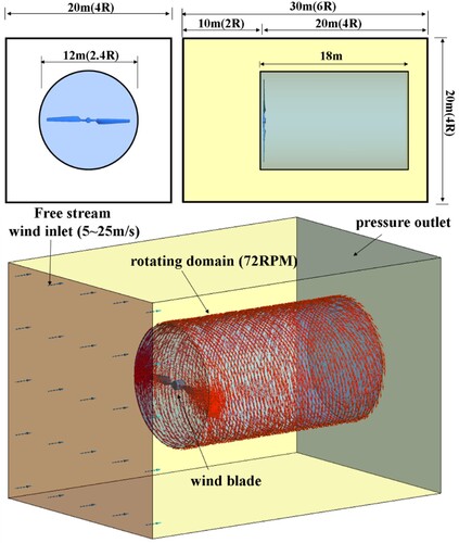
In our study, as shown in Figure 3, the best compromise for the computational domain of the wind turbine blades has a height of 20 m, a width of 20 m, and a length of 30 m in the streamwise direction. The domain includes two parts: the interior rotary domain (cylindrical part that includes the blades) with a high mesh density and the external stationary domain (wind tunnel part) with a low mesh density.

Figure 3. Computational domain definition and dimension.

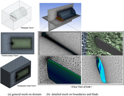
Unstructured grids with approximately 14 million elements and 3.7 million nodes were created for the CFD simulation. The refined cell, which is approximately 0.0001 m in length, is distributed near the blade surface, and the grid volume is gradually coarsened approaching the far-field region so that the grid quantity and the computational time can be relatively reduced. The minimum mesh orthogonal quality is approximately 2.08 × 10^–5 with a growth rate of 1.15. The optimal compromised grids for the computational mesh at different boundaries are shown in Figure 4. Furthermore, to deal with the boundary effect, 18 inflation layers are constructed around the boundary wall, and refinement is made to satisfy y + ≤1.

Figure 4. General and detailed computational mesh. (a) General mesh on domain; (b) detailed mesh on boundaries and blade.

The boundary conditions (BCs) of the domain were defined as follows: the front face of the cuboid is defined as a wind inlet type BC, the back surface of the box is defined as a pressure outlet type BC, and a symmetry type BC is applied to the lateral surface of the box. In all cases, uniform velocity normal to the inlet is utilised at the wind inlet boundary with a medium turbulent intensity of 5%, and atmospheric static pressure is applied at the outlet and far-field boundaries. For turbulence calculations, SST Gamma theta model has been implemented. The SST Gamma Theta model is a four-equation turbulent-transitional model that includes the SST turbulent model and the Gamma Theta transitional model. The idea behind the SST turbulent model is combining the advantages of the k–ϵ and k–ω models by utilising the first blending function F₁. The word ‘blending’ indicates that both the models are taken into consideration; F₁ is equal to 1 near the blade surface to activate the k–ω model and 0 in the rest of the flow to activate the k–ϵ model. SST Gamma theta transitional turbulent model (Menter 1994; Menter 2009; Langtry and Menter 2005; Menter, Langtry, and Völker 2006a; Menter et al. 2006b; Menter et al. 2003) complements transport of the turbulent shear stress with a modified eddy viscosity equation that provides higher accuracy and reliability while also maintaining stability. This model yields much more accurate simulations around the aerofoil surface, especially in the separation region. This model can be expressed as below: $\begin{array}{rl}& {\displaystyle \frac{\mathrm{\partial }\rho k}{\mathrm{\partial }t}+{\displaystyle \frac{\mathrm{\partial }(\rho U_{j}k)}{\mathrm{\partial }{x}_j}=\left(min\left({\tau }_{ij}{\displaystyle \frac{\mathrm{\partial }{U}_i}{\mathrm{\partial }{x}_j}{c}_l\epsilon }\right)\right)-{\beta }^{\ast }\rho \omega k+{\displaystyle \frac{\mathrm{\partial }}{\mathrm{\partial }{x}_j}\left[\left(\mu +{\displaystyle \frac{{\mu }_t}{{\sigma }_k}}\right){\displaystyle \frac{\mathrm{\partial }k}{\mathrm{\partial }{x}_j}}\right]}}}\\ & {\displaystyle \frac{\mathrm{\partial }\rho \omega }{\mathrm{\partial }t}+{\displaystyle \frac{\mathrm{\partial }(\rho U_j\omega )}{\mathrm{\partial }{x}_j}={\displaystyle \frac{\gamma }{v_t}{\tau }_{ij}{\displaystyle \frac{\mathrm{\partial }{U}_i}{\mathrm{\partial }{x}_j}-\beta \rho {\omega }^2+{\displaystyle \frac{\mathrm{\partial }}{\mathrm{\partial }{x}_j}\left[\left(\mu +{\displaystyle \frac{{\mu }_t}{{\sigma }_{\omega }}}\right){\displaystyle \frac{\mathrm{\partial }\omega }{\mathrm{\partial }{x}_j}}\right]+2\rho (1-{\mathrm{F}}_1){\sigma }_{\omega 2}{\displaystyle \frac{1}{\omega }{\displaystyle \frac{\mathrm{\partial }k}{\mathrm{\partial }{x}_j}{\displaystyle \frac{\mathrm{\partial }\omega }{\mathrm{\partial }{x}_j}}}}}}}}}\end{array}$where, $\begin{array}{rl}& F_1=\tanh \left({\left(min\left(max\left({\displaystyle \frac{\sqrt{k}}{{\beta }^{\ast }\omega y}{\displaystyle \frac{500\upsilon }{y^2\omega }}}\right){\displaystyle \frac{4\rho {\sigma }_{\omega 2}}{C{D}_{k\omega }{y}^2}}\right)\right)}^4\right)\\ & C{D}_{k\omega }=max\left(2\rho {\sigma }_{\omega 2}{\displaystyle \frac{1}{\omega }{\displaystyle \frac{\mathrm{\partial }k}{\mathrm{\partial }{x}_j}{\displaystyle \frac{\mathrm{\partial }\omega }{\mathrm{\partial }{x}_j}1.0e^{-10}}}}\right)\end{array}$$\rho$: Density; k: the turbulent kinetic energy; $\epsilon$: dissipation rate; $\mu$: molecular viscosity;

${\mu }_t$: The eddy or turbulent viscosity; $\tau$: wall shear stress; $\omega =$ specific turbulence dissipation rate; ${\sigma }_{k1}=2$; ${\sigma }_{\omega 1}=2.000$; $\kappa =0.41$; ${\gamma }_1=0.5532$; ${\beta }^{\ast }=0.09$; ${\beta }_1=0.075$; $c_l=10$; ${\sigma }_{k2}=1$; ${\sigma }_{\omega 2}=1.168$; $\kappa =0.41$; ${\gamma }_2=0.4403$; ${\beta }^{\ast }=0.09$; ${\beta }_2=0.0828$.

The new relationship of constant parameter with the k– ϵ and the k– ϵ model is [8]: $\varphi =F_1{\phi }_1+(1-F_1){\phi }_2$where ${\phi }_1,{\phi }_2$ are the coefficients of the k–ϵ and the k–ϵ model, respectively [8]:

Furthermore, to restrict the shear stress in the wall boundary layer and obtain the onset of separation correctly, the eddy viscosity is modified by introducing second blending function F2 [8–10]: ${\mu }_t={\displaystyle \frac{\rho a_{1}k}{max\left({\alpha }_1\omega ,\sqrt{2}\mathrm{S}{\mathrm{F}}_2\right)}}$where, $\mathrm{Constant}{a}_1=0.31F_2=\tanh \left({\left(max\left({\displaystyle \frac{2\sqrt{k}}{{\beta }^{\ast }\omega y}{\displaystyle \frac{500\upsilon }{y^2\omega }}}\right)\right)}^2\right)$More information about this model, its verification and application can be found in the work of Menter and Langtry.

4. Results and discussion

In this study, the sectional pressure coefficients C_P and blending functions were first analysed. Subsequently, the intermittency, transition onset Reynolds number, and streamlines on both the suction and pressure surfaces of the blade were explained. Furthermore, the tangent force and normal force coefficients (C_T and C_N, respectively) in the five sections were investigated and explained. Finally, the results of torque and thrust on the entire blade were determined and compared with various turbulent model results.

4.1. Stall definition

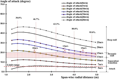
Based on the experimental results from 2D wind tunnel test in the Ohio State University (Ramsay, Hoffmann, and Gregorek 1995), C_L and C_D for the S809 aerofoil versus the AOA were identified (Lee et al., 2016b, 2017; Roy et al. 2017). In this study, the AOA ranging from −6° to 6° is regarded as the Attached Flow Region, where C_L and C_D vary almost linearly with AOA, and the main flow behaviour is an attached flow. The region where the AOA is approximately 6°–15° is termed as Separation/Transition Region. A mixed flow behaviour of attached, separated, and transitional flow on the blade surface may happen in the Separation/Transition Region. At around 15° AOA, which yields the maximum C_L value and marks the beginning of the Dynamic Stall Region, is defined as the critical AOA in this 2D S809 aerofoil case. At around 20° AOA, a sudden change in C_L and C_D occurs, and the region shifts from Dynamic Stall Region to Deep Stall Region. After the 20° AOA, the airflow separates right after the leading edge, and fully separated flow on the suction surface can be observed. Many researchers have discussed the importance of the 20° AOA (Tangler and Kocurek 2005). In the current work, 20° AOA is regarded as the Onset of the Fully Separated flow and is also used to explain the flow behaviours on the wind turbine blade surface. In addition, the dynamic stall and deep stall regions are combined together and defined as the Post-stall Region, where stall starts to appear.

The 3D AOA distributions for the NREL Phase VI blade versus the spanwise radial distance at different wind speeds are illustrated in Figure 5. It is known that separation and transition can happen even though attached flow is still dominant at low AOA. For the case with a wind speed of 5 m/s, the attached flow prevails, but a little separation and transitional flow could also happen because small part of blade span is above the attached region. At a wind speed of 7 m/s, all sections are in the separation/transition region. Thus, a small separation or transition combined with a largely attached flow could be observed there. The AOA of 15°–20° is defined as dynamic stall region, and three wind speed cases (10–15 m/s) pass through it. In particular, 10 m/s case can be regarded as the stall onset velocity since it is the first case that passes through the dynamic stall region. A mixed flow behaviour of attached, transitional and turbulent flow is expected to be found in these three cases. As shown in Figure 5, the location where 20° AOA occurs in 10 m/s case is around 45.0% section, around 70.0% spanwise radius in 13 m/s and 90.0% section in 15 m/s case, respectively. Thus, the separation region size in these three cases would increase as the wind speed increases whereas the attached region decreases. Finally, 20 and 25 m/s cases are in the deep stall region and the flow is totally separated, as their AOA from tip to root are higher than 20°.

Figure 5. Relationship for angle of attack in span-wise with different wind speed.

4.2. Blending function and pressure coefficient

The separation and transition that occur in the boundary layer with SST Gamma Theta model by analysing the blending functions, intermittency, and transition onset Reynolds number (Figures 6–14) are presented in this section. The separation and transition have a strong effect on the near-wall behaviour. The capability of the SST turbulent model to predict separated flow has been demonstrated in many previous studies (Mo and Lee 2012; Moshfeghi, Song, and Xie 2012; Lanzafame, Mauro, and Messina 2013; Yelmule and Vsj 2013). Figures 6–9 show the sectional pressure coefficient, velocity coefficient contours, and blending function contours around the sectional aerofoils on the span-wise sections r/R = 30.0%, 46.7%, 63.3%, 80.0%, and 95.0% with several wind velocities ranging from 5, 10, 15, and 20 m/s. From Figures 6–9, it can be observed that for all velocity coefficient contours, changes occur primarily on the suction surface of the aerofoil, which indicates that more attention is required on suction surface during analysis. In addition, for the first blending function of SST model, the red contour expresses that the k–ω model is applied in the boundary layer region, whereas the dark blue contour shows the application of the k–ω model in the freestream. For the second blending function, the distribution of the turbulent shear stress near the wall for an aerofoil is shown, which corrects the overestimated eddy viscosity of the boundary layer in F₁. Moreover, for the transitional blending function, the red contour near the wall shows the place where the source term is turned off in the boundary layer whereas the yellow and dark blue contours show the place where the transported scalar is diffused from the free stream to match the local value and where transition occurs. For pressure coefficient, a comparison is made between the CFD results, and the experimental data obtained from the pressure tabs installed in the blade.

Figure 6. Sectional coefficients and blending functions contours for 5 m/s wind speed case. (a) Blending functions: 5 m/s wind speed case; (b) Pressure coefficients and velocity coefficient contours: 5 m/s wind speed case.

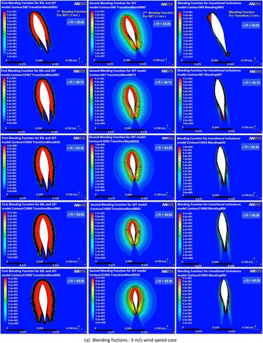
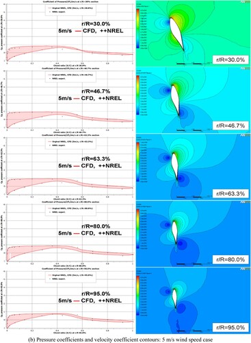
Figure 7. Sectional coefficients and blending functions contours for 10 m/s wind speed case. (a) Blending functions: 10 m/s wind speed case; (b) Pressure coefficients and velocity coefficient contours: 10 m/s.

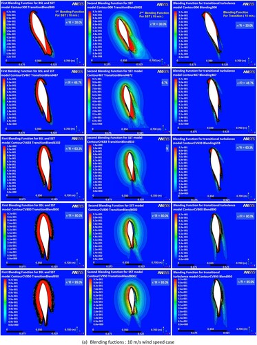
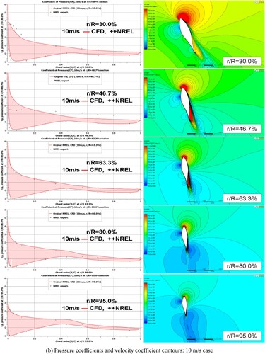
Figure 8. Sectional coefficients and blending functions contours for 15 m/s wind speed case.

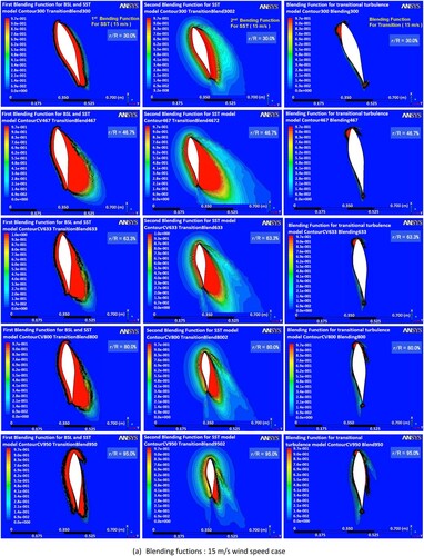
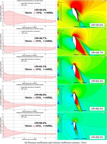
Figure 9. Sectional coefficients and blending functions contours for 20 m/s wind speed case.

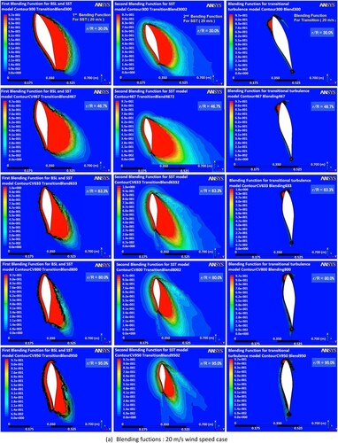
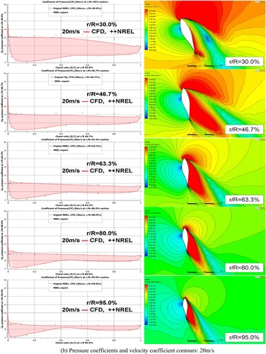
Figure 10. Turbulence intermittency on the suction and pressure side for five different wind speed cases. (a) Turbulence intermittency of the suction side for five different wind speed cases; (b) Turbulence intermittency of the pressure side for five different wind speed cases.

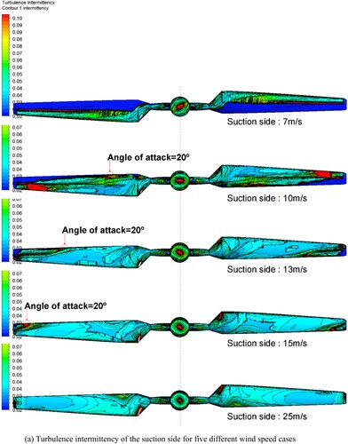
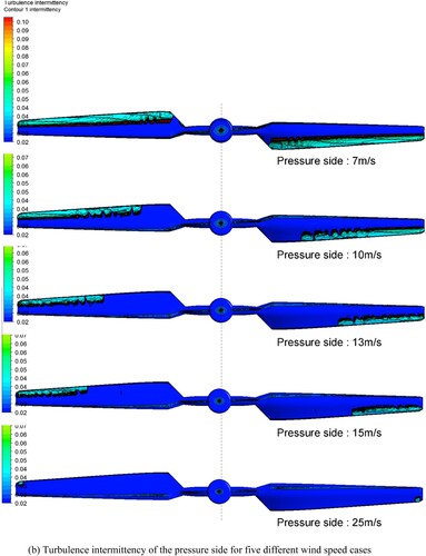
Figure 11. Transition onset Reynolds number on the suction and pressure side for five different wind speed cases. (a) Transition onset Reynolds number of the suction side for five different wind speed cases; (b) Transition onset Reynolds number of the pressure side for five different wind speed cases.

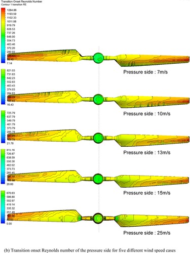
Figure 12. Tangential and normal force coefficient with pressure coefficient for different velocities. (a) Aerodynamic coefficient for 5 m/s wind speed case; (b) Aerodynamic coefficient for 7 m/s wind speed case; (c) Aerodynamic coefficient for 10 m/s wind speed case; (d) Aerodynamic coefficient for 13 m/s wind speed case; (e) Aerodynamic coefficient for 15 m/s wind speed case; (f) Aerodynamic coefficient for 20 m/s wind speed case; (g) Aerodynamic coefficient for 25 m/s wind speed case.

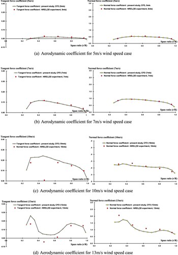
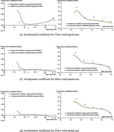
Figure 13. Comparison of torque value between different simulation approaches with NREL data.

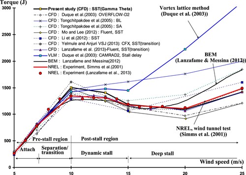
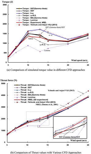
Figure 14. Comparison of thrust and torque with different turbulence models. (a) Comparison of simulated torque value in different CFD approaches; (b) Comparison of thrust values with various CFD approaches.

In 5 m/s case (Figure 6), for the first blending function, most of the aerofoil surface region in the whole blade is governed by the k–ω model whereas a little part of surface region in the trailing edge is by the k–ω model. The reason is that with the increase of the turbulence intensity near the trailing region, the value of F₁ decreases which introduces the k–ω model. For the second blending function, the red contour on both the suction and pressure surfaces of the entire section decreases in size, which corrects the boundary layer predictions in F₁. Weak separation might occur around the middle span of the aerofoil along the blade. Transitional flow can be verified from the transitional blending function. It is found that wake contours on both surfaces appear near the middle chord position of the last four sections (r/R = 46.7% to 95.0%), which indicates the position of the transitional flow. The velocity coefficient contours in five sections through the contour lines intersecting the surface, indicate that the whole blade in 5 m/s case is mainly in the attached flow behaviour whereas very weak separation or transition is observed between the half of the chord position and the trailing edge, which satisfies the expectations in Figure 5 as well as the prediction in blending functions. Then, the C_P value for five sections can be calculated from the above-obtained velocity coefficient contour. The calculated C_P value is in good agreement with the measured experimental data for all spanwise sections.

The 10 m/s wind speed is a critical case where stall first appears as defined in Figure 5. In the 10 m/s case (Figure 7), for the first blending function, the k–ω model at the leading edge of the suction surface continues decreasing in size in the range of r/R = 60.0%–95.0% span. However, the k–ω model governs the trailing edge instead of the leading edge in the 30.0% and 46.7% sections. Comparing with the second blending function, overestimation on the boundary layer in F₁ is observed for the whole blade of the pressure surface as well as the leading edge of the suction surface in the range of r/R = 63.3%–95.0% sections. For the suction surface of the first two sections (r/R = 30.0%, 46.7%), underestimation of the boundary layer in the leading edge is found. The separation is observed at the leading edge of the first section and transfers to the trailing edge as the section r/R ratio increases. It reaches around the middle of the aerofoil at the fifth section (r/R = 95.0%). For the pressure surface of the transitional blending function, transition occurs mainly in the region between middle span and the trailing edge near the hub. However, on the suction surface, no transition is found in the first section (r/R = 30.0%). From the span ratio of r/R = 46.7%–95.0%, transition occurs in the leading edge and spreads to the middle span as the span ratio increases. This result satisfies the predictions in Figure 5, which shows that before the 46.7% span section, the blade is in the deep stall region and the remainder of the sections are in the separation/transition region. From velocity coefficient contours, it is found that separation occurs in the suction surface at the span ratio of 30.0% whereas separation or separation-induced transition moves towards the trailing edge of the suction surface as the span ratio increases. For the calculated C_P values, discrepancies were observed near the leading edge of the suction surface, and these discrepancies are mainly located in the first two sections, especially at the 46.7% span. The reason for this is that radial flow resulting from centrifugal acceleration may change the distribution of the blade pressure when the blade rotates (Lanzafame and Messina 2012) . Flow separation and induced stall-delay effects can make the suction pressure more difficult to be accurately captured in this simulation than in the experiments (Schreck, Hand, and Fingersh 2001; Hand et al. 2001). In addition, the regions close to the complicated hub geometry may cause some deviation between the measured and simulated results.

In the 15 m/s case (Figure 8), for the first blending function, the whole aerofoil surface in the first four sections (r/R = 30.0%–80.0%) is governed by the k–ω model whereas a little part near the leading edge on the suction side of the 95.0% ratio section is by k–ω model. Likewise, for the second blending function, similar boundary layers are predicted in the first four sections but with an intensive pattern. The main difference between F₁ and F₂ is located in the 95.0% section where F₁ overestimates the boundary layer on the pressure surface and the leading edge of the suction surface. It can be found that the whole suction surfaces of the first four sections were totally separated. For the fifth section (r/R = 95.0%), the separation starts at around 30.0% chord position. For the transitional blending function, weak transition can be found near the middle span to the trailing edge region of the last three sections (r/R = 63.3%–95.0%) on the pressure surface whereas on the suction surface, it occurs near the leading edge of the tip region. For the velocity coefficient contours, clear separation on the whole suction surface is observed in the first four sections (in the span ratio from r/R = 30.0%–80.0%). It diminishes when flow proceeds in chordwise direction. Since separation also diminishes in the spanwise direction, weak separation is found near the middle span of the 95.0% section. As shown in Figure 5, the region including the 30.0%–80.0% spanwise sections was in the deep stall region, and the last span (95.0%) was in the dynamic stall region. Therefore, prediction from blending functions and velocity contour are in good agreement with Figure 5. The overall calculated C_P values show good agreement with the NREL experimental data, though small difference exists, like the overestimation of C_P on the leading edge of the 30.0% section. One possible reason that may explain this inboard inconsistency is that the blade may have undergone a stall effect due to the large AOA. It can be observed in Figure 5 that the AOA near the hub is around 30° and is in the deep stall region.

Finally, in the 20 m/s case (Figure 9), all five sections are governed by k–ω model for the first blending function. The intensity of k–ω model contour is found to be stronger. Similar contours are also obtained in the second blending function. It is found that the whole suction surface of 20 m/s case is totally separated. This can also be verified from the transitional blending function, since no transition is observed in the suction surface of this case whereas very weak transition is observed in the pressure surface. In addition, in the velocity coefficient contour, clear separation starting from the leading edge can be observed in this case. This is in good agreement with the prediction from Figure 5, which indicates that the whole blade in the 20 m/s case would be in the deep stall region and the flow would be fully turbulent across the whole blade span. Although a little difference in the C_P values exists, the C_P values obtained in this study show good agreement with the experimental values. These discrepancies might be caused by unsteady flow, and the stall effect which may have resulted from the high AOAs since all the sections in this case exceed 30°. Moreover, very desirable results can be obtained when integrating the pressure for the whole blade surface. It was found that all the results of the first blending function were rarely consistent with those of the second blending function. Furthermore, even though similar results were occasionally obtained from the first and second blending functions, such as in high wind speed case (20 m/s), it should also be noted that differences in the contours still exist. With the increase of the wind speed, the transition and separation position diminish from the hub to tip. Finally, with the help of the first, second, and transitional blending functions and the AOA distributions on the 3D blade, a clear understanding of the pressure coefficient was provided.

4.3. Turbulence intermittency and transition onset Reynold number

To have an advanced investigation on transitional flow, predicted turbulence intermittency, and transition onset Reynold number on both the suction and pressure sides for five different wind speed cases (7, 10, 13, 15, 25 m/s) are presented in Figures 10 and 11. For turbulence intermittency, the dark blue contour shows the attached flow region while the light blue contour presents the separated flow region and the red contour represents the transitional flow region. For and transition onset Reynold number, the dark blue contour shows the separated flow region whereas the yellow contour presents the attached flow region and the region between these two represents the transitional flow region.

For the suction side of the 7 m/s wind speed case (Figure 10(a)), the flow is largely attached. In particular, a significant amount of laminar flow is predicted from the leading edge to half of the chord position of the whole blade. Transition occurs at the 50.0% chord position along almost the entire blade surface. For the 10 m/s case, the inner hub region stalls. The tip region remains attached, and the laminar flow region decreases from the 50.0% chord position to the leading edge. The marked 20° AOA at the leading edge shows clear separation which is in accordance with the definition in Figure 5. Comparing with 7 m/s case, the transition location moves to the leading edge. With the increase of the wind speed, separation on the blade surface became robust. For 15 m/s case, the attached region continues decreasing in size and occurs around 95.0% spanwise ratio. The onset of the separation at the leading edge is around in 90.0% spanwise and from this point extending to the half chord at the tip is the transitional region. Finally, at 25 m/s the intermittency contours indicate that the flow is almost completely separated.

For the pressure surface (Figure 10(b)), attached flow is dominant in four higher speeds out of five speed cases. For 7 m/s case, the separated region is from the leading edge to the range of around 40.0% chord length of almost the whole blade. The transitional region located in 40.0% chord length from the hub to tip of the blade surface. As the increase of the wind speed, the separated and transitional region decreased in term of size. Therefore, in 15 m/s case, the transitional region is from around 65.0% spanwise ratio to the tip in 20.0% chord position. Finally, in 25 m/s case, the flow is mainly attached at the pressure surface.

Figure 11 presents the predicted transition onset Reynolds number for four wind speeds. For suction side of 7 m/s case, attached flow is dominant and transitional flow can be observed around the middle of the chord position along the blade. As the wind speed increases, the effective angle of attack of the wind turbine blade also increases. For 10 m/s case, the separated flow is dominant and it governs the hub region as well as the trailing edge part of the rest of the blade. Transition occurs in the 50.0% chord position of the tip and extends to the leading edge near the hub. Clear separation at the leading edge can be found in the 20° AOA, as defined in Figure 5. In 15 m/s case, the size of laminar flow contour continues decreasing and attached flow is observed up to the 0.5 chord position in the tip region. Due to the increased angle of attack, the transition location near the tip moves to the leading edge. Finally, at 25 m/s, dark blue contour was found on the entire surface which means that the suction side of the blade is totally separated. For the pressure side, all the blade surfaces of the transition onset Reynolds number for four wind speed cases are similar: laminar flow is the main flow behaviour and weak transition is observed in the middle chord near tip region. With the increase of the wind speed, the transitional contour diminishes towards the tip region. Notice good consistency can be achieved, when comparing with the transitional flow predictions from transitional blending function, which in turn verifies the prediction for the near wall flow transition behaviours.

4.4. Tangent and normal force coefficient simulation

The normal and tangent force coefficients (C_N and C_T, respectively) demonstrate the forces acting vertical to the aerofoil chord line and parallel to the aerofoil chord, respectively. They can be calculated by integrating the average pressure of two adjoining positions that are projected onto the chord and onto an axis orthogonal to the chord, respectively. Thus, separation on the suction surface can have a huge influence on the value of C_T whereas little influence on C_N. The evaluation of these aerodynamic parameters allows further verification of the SST Gamma Theta model and the previous predictions of the blending functions, intermittency and transition onset Reynolds number. Notice the experimental data are limited to only five sections, with locations of r/R = 30.0%, 46.7%, 63.3%, 80.0%, and 95.0%. However, CFD simulation results in this study are obtained in 16 sections to get smoother trends. Results for four wind speeds, 7, 10, 15, and 20 m/s are presented in Figure 12.

For the 7 m/s wind speed, as shown in Figure 12(a), the CFD results of the C_T and C_N values for the entire blade agree well with the NREL experimental data, despite separation appearing in the root. This is consistent with the previously obtained accurate C_P values. This also proved the accuracy of our CFD simulation model.

As the wind speed increases, the separated flow became stable, clear, and important, and discrepancies appeared gradually. As shown in Figure 12(b), for 10 m/s, except in the 46.7% span section where a sudden dip occurs in NREL results while flat contour value is observed in CFD results, C_T values are found to be in good agreement with the NREL experimental data. It should be noted that the critical 20° AOA, which indicates the onset of the total separation on the leading edge, is also located near the 46.7% span section. Therefore, the predicted high C_T value may have resulted from the inaccuracy of the C_P results, which is caused by the stall delay phenomenon. For the C_N value of 10 m/s case, no sudden decrease but smooth value change is observed in both CFD results and the NREL experimental results. The reason is that C_N is less affected by suction surface separation or stall phenomena. So good agreement between CFD results and NREL data is obtained.

For 15 m/s wind speed, the calculated C_T and C_N results showed trends similar to the experimental data. These two cases are in the dynamic stall region. The drag force in the tip region of the blade increases whereas the lift force decreases, which induced a decreased trend in C_N value. Other part of the blade is in the deep stall region which is totally separated and had little influence on the C_N value. The stall delay effect, occurred in 10 m/s case of C_T results, does not show here. Therefore, good agreement between this study and NREL experimental values is achieved whereas small differences are observed. These differences might be caused from the discrepancies in the suction surface leading edge of the C_P results where separation happened.

For the fully separated case of 20 m/s wind speed, CFD calculated C_T and C_N results match the NREL results well with all the blade sections whereas small differences are observed. This can also be found in the C_P results. In the post-stall region from 10 to 20 m/s, the C_T curves were slightly higher than the NREL results, which were affected by the separation, but the overall trends are in good agreement with the experimental results.

It is known that the SST Gamma Theta model is capable of providing accurate predictions for separation and transition. The calculated results of the aerodynamic force coefficients show comparatively good agreement with the NREL experimental data, even though small discrepancies exist. In every wind speed case, data from 16 sections were collected in this study instead of five sections, as was used in the NREL test. Thus, the simulation results yielded smoother aerodynamic force coefficient curves.

4.5. Torque and thrust analysis

A comparative study of the SST Gamma Theta model with the other turbulent models in calculating the aerodynamic characteristics of the NREL Phase VI wind turbine blade was performed and are shown in Figures 13 and 14. Various turbulent models were adopted to calculate the torque and thrust under the same grid and simulation conditions. SST-based turbulent models present trends similar to those of the experimental data. In particular, better consistency with the NREL 3D experimental torque results was achieved in the SST Gamma Theta and SST models than with other turbulent models, including the k–ω, BSL, and ω–R.S. model (omega-based Reynolds stress model), etc. For the torque value of the whole blade, results from SST model and SST Gamma Theta model are very similar, both of them show very accurate results. Differences with the NREL experimental data are observed in k–ω, BSL Gamma Theta and ω-R.S. models. The underestimation in the ω-R.S. model resulted from too fine resolution. For k–ω model, it is substantially accurate in the near wall layers but fails in the free stream region outside the boundary layer. This disadvantage is reduced in BSL model with the help of the first blending function. However, discrepancies still exist since neither of these two models consider the turbulent shear stress. Therefore, SST turbulence model is developed to take the turbulence shear stress into account by modifying the eddy viscosity and introducing the second blending function. As described in many papers (Moshfeghi, Song, and Xie 2012; Lanzafame, Mauro, and Messina 2013; Yelmule and Vsj 2013; Menter 1994, 2009; Menter et al. 2003), the SST turbulent model is already known to be able to consider the inner sublayer of the wall, properly predict the separation, and provide accurate results under adverse pressure gradient. For SST Gamma Theta model, as mentioned previously, it has the capability to accurately predict the onset and the length of transition, however, shaft torque value of the blade is more affected by separation instead of transition. Thus, both of these two models show accurate predictions.

For all of the models in Figure 14, the calculated thrust force values agree well with the experimental data. And there are little discrepancies between turbulent models except lamina model and Yelmule and Vsj (2013) result. Thrust force is mainly related to the C_N and thus little affected by separation. Good results in C_N make it possible to achieve accurate thrust force in SST-based model. Thrust calculated from the SST turbulent and SST Gamma Theta models are very similar in all cases. Minor discrepancies (errors deemed acceptable, as all were less than 5%) were observed in the post-stall region (10–20 m/s). the maximum deviation happened in 15 m/s, and could be interpreted as the natural inability of the SST turbulence model to predict the separation point in highly separated flows (Moshfeghi, Song, and Xie 2012).

As demonstrated above, the calculated torque and thrust force from the SST Gamma Theta method, agree well with the experimental data. Thus, the ability of this model to identify separation and transition is verified, and it can be applied to simulate other aerodynamic parameters of the blade in the future work.

5. Conclusions

In this study, complex separated and transitional flows at the boundary layer of the NREL Phase VI wind turbine blade were analysed by utilising the SST Gamma Theta model. The near wall flow behaviour was predicted using a newer approach: blending functions, intermittency, and transition onset Reynolds number. The success and accuracy of the aerodynamic force prediction through blending function are validated with the streamline flow simulations. It was observed that on the suction surface, attached flow was predominant and a slight transitional flow occurred when the flow speed was low (5 m/s). As the speed increased to 7 m/s, separated flow first appeared near the hub, and the transitional flow in the radial direction became relatively clear. As the wind velocity increased further, the separation progressively spread from the hub to the tip and also from the trailing edge to the leading edge, ultimately covered the entire blade at 20 and 25 m/s, where the flow was fully turbulent across the whole span.

Using this strategy, the locations of separated and transitional flows on the blade surface were analysed successfully. Other aerodynamic parameters, including pressure coefficient, normal and tangent force coefficients, thrust, and torque, were evaluated, compared with the experimental data, and shown to be in good agreement. As a result, the SST Gamma Theta model using blending functions, intermittency, and transition onset Reynolds number to explain the flow characteristics of separation and transition was proven to be a better and more accurate approach. This newer approach to predict aerodynamic flow provides numerical computation to be more powerful and reliable. In future research, this flow visualisation will help to identify more complex phenomena of turbulence and transition intermittency for different aerodynamic load and blade design conditions. In the future, our results will be applied to fluid structure interaction.

Disclosure statement

No potential conflict of interest was reported by the author(s).

Additional information

Funding

This research was supported by the National Science Foundation (NSF) through the Center for Energy and Environmental Sustainability (CEES), a CREST Center (Award No. 1036593).

References

- Dai, J., Y. Hu, D. Liu, and X. Long. 2011. “Aerodynamic Loads Calculation and Analysis for Large Scale Wind Turbine Based on Combining BEM Modified Theory with Dynamic Stall Model.” Renewable Energy 36: 1095–1104.
- Duque, E.P.N., M.D. Burklund, and W. Johnson. 2003. “Navier-Stokes and Comprehensive Analysis Performance Predictions of The NREL Phase VI Experiment.” Journal of Solar Energy Engineering 125: 457–467. doi:10.1115/1.1624088.
- Hand, M., D. Simms, L.J. Fingersh, D. Jager, S. Schreck, and S.M. Larwood. 2001. “Unsteady Aerodynamics Experiment Phase VI: Wind Tunnel Test Configurations and Available Data Campaigns.” National Renewable Energy Laboratory (NREL) Technical Report NREL/TP-500-23955.
- Langtry, R.B., and F.R. Menter. 2005. “Transition Modeling for General CFD Applications in Aeronautics.” American Institute of Aeronautics and Astronautics (AIAA) 2005-522.
- Lanzafame, R., S. Mauro, and M. Messina. 2013. “Wind Turbine CFD Modeling Using a Correlation-Based Transitional Model.” Renewable Energy 52: 31–39. doi:10.1016/j.renene.2012.10.007.
- Lanzafame, R., and M. Messina. 2012. “BEM Theory: How to Take Into Account the Radial Flow Inside of a 1-D Numerical Code.” Renewable Energy 39: 440–446. doi:10.1016/j.renene.2011.08.008.
- Lee, K., Z. Huque, R. Kommalapati, and H.S. Eul. 2016a. “Evaluation of Equivalent Structural Properties of NREL Phase VI Wind Turbine Blade.” Renewable Energy 86: 796–818. doi:10.1016/j.renene.2015.07.096.
- Lee, K., Z. Huque, R. Kommalapati, S. Roy, C. Sui, and N. Munir. 2016b. “Aerodynamic Noise Characteristics of Horizontal Axis Wind Turbine Blade Using CAA.” Journal of Clean Energy Technologies 4 (5): 346–352. doi:10.18178/JOCET.2016.4.5.310.
- Lee, S.G., S.J. Park, K.S. Lee, and C. Chung. 2012. “Performance Prediction of NREL (National Renewable Energy Laboratory) Phase VI Blade Adopting Blunt Trailing Edge Airfoil.” Energy 47: 47–61. doi:10.1016/j.energy.2012.08.007.
- Lee, K., S. Roy, Z. Huque, R. Kommalapati, and S.E. Han. 2017. “Effect on Torque and Thrust of the Pointed Tip Shape of a Wind Turbine Blade.” Energies 10: 79. doi:10.3390/en10010079.
- Li, Y.W., K.-J. Paik, T. Xing, and P.M. Carrica. 2012. “Dynamic Overset CFD Simulations of Wind Turbine Aerodynamics.” Renewable Energy 37: 285–298. doi:10.1016/j.renene.2011.06.029.
- Menter, F.R. 1994. “Two-Equation Eddy-Viscosity Turbulence Models for Engineering Applications.” AIAA Journal 32(8): 1598–1605.
- Menter, F.R. 2009. “Review of the Shear-Stress Transport Turbulence Model Experience from an Industrial Perspective.” International Journal of Computational Fluid Dynamics 23: 305–316. doi:10.1080/10618560902773387.
- Menter, F., J.C. Ferreira, T. Esch, and B. Konno. 2003. “The SST Turbulence Model with Improved Wall Treatment for Heat Transfer Predictions in Gas Turbines.” The International Gas Turbine Congress, Tokyo.
- Menter, F.R., R.B. Langtry, S.R. Likki, Y.B. Suzen, P.G. Huang, and S. Völker. 2006b. “A Correlation-Based Transition Model Using Local Variables Part I: Model Formulation.” Journal of Turbomachinery 128: 413–422. doi:10.1115/1.2184352.
- Menter, F.R., R. Langtry, and S. Völker. 2006a. “Transition Modeling for General Purpose Codes.” Journal Flow Turbulence and Combustion 77: 277–303. doi:10.1007/s10494-006-9047-1.
- Mo, J., A. Choudhry, M. Arjomandi, R. Kelso, and Y.H. Lee. 2013. “Effects of Wind Speed Changes on Wake Instability of a Wind Turbine in a Virtual Wind Tunnel Using Large Eddy Simulation.” Journal of Wind Engineering and Industrial Aerodynamics 117: 38–56. doi:10.1016/j.jweia.2013.03.007.
- Mo, J.O., and Y.H. Lee. 2012. “CFD Investigation on the Aerodynamic Characteristics of a Small-Sized Wind Turbine of NREL PHASE VI Operating with a Stall-Regulated Method.” Journal of Mechanical Science and Technology 26: 81–92. doi:10.1007/s12206-011-1014-7.
- Moshfeghi, M., Y.J. Song, and Y.H. Xie. 2012. “Effects of Near-Wall Grid Spacing on SST-K-ω Model Using NREL Phase VI Horizontal Axis Wind Turbine.” Journal of Wind Engineering and Industrial Aerodynamics 107-108: 94–105. doi:10.1016/j.jweia.2012.03.032.
- Potsdam, M.A., and D.J. Mavriplis. 2009. “Unstructured Mesh CFD Aerodynamic Analysis of the NREL Phase VI Rotor.” In 47th AIAA Aerospace Sciences Meeting, Orlando, FL, USA.
- Ramsay, R.R., M.J. Hoffmann, and G.M. Gregorek. 1995. “Effects of Grit Roughness and Pitch Oscillations on the S809 Airfoil.” In Airfoil Performance Report NREL/TP-442-7817.
- Roy, S., Z. Huque, K. Lee, and R. Kommalapati. 2017. “Turbulence Model Prediction Capability in 2D Airfoil of NREL Wind Turbine Blade at Stall and Post Stall Regions.” Journal of Clean Energy Technologies 6 (6): 496–500. doi:10.18178/JOCET.2017.5.6.423.
- Schreck, S., M. Hand, and L.J. Fingersh. 2001. “NREL Unsteady Aerodynamics Experiment in the NASA-Ames Wind Tunnel: A Comparison of Predictions to Measurements.” National Renewable Energy Laboratory (NREL) Technical Report NREL/TP-500-29494.
- Sezer-Uzol, N., and L.N. Long. 2016. “3-D Time-Accurate CFD Simulations of Wind Turbine Rotor Flow Fields.” In 44th AIAA Aerospace Sciences Meeting and Exhibit, Reno, Nevada.
- Sharifi, A., and M.R.H. Nobari. 2013. “Prediction of Optimum Section Pitch Angle Distribution Along Wind Turbine Blades.” Energy Conversion and Management 67: 342–350. doi:10.1016/j.enconman.2012.12.010
- Tangler, J.L., and J.D. Kocurek. 2005. “Wind Turbine Post-stall Airfoil Performance Characteristics Guidelines for Blade-Element Momentum Methods.” In 43rd AIAA Aerospace Sciences Meeting and Exhibit. Reno, Nevada: NREL/CP-500-36900.
- Yelmule, M.M., and E.A. Vsj. 2013. “CFD Predictions of NREL Phase VI Rotor Experiments in NASA/AMES Wind Tunnel.” International Journal of Renewable Energy Research 3(2): 261–269.