A reliability-constrained optimisation framework for offshore wind turbine support structures

ABSTRACT

A new approach that links finite element analysis (FEA) and a genetic algorithm (GA) with Monte Carlo simulation (MCS) for the reliability-constrained optimal design of offshore wind turbine (OWT) support structure is presented. This approach has been applied to optimise the NREL 5MW OWT on OC3 support structure. The objective function minimises the weight of the support structure, constrained to design and performance limits, by attaining the desired reliability level. A response analysis of the reference OWT is performed to estimate design loads. Then, deterministic optimisation (DO) is carried out to find the candidate design solutions. After that, a reliability assessment is conducted to apply the target reliability constraint. This study reveals that the design of a monopile support structure is mainly driven by fatigue limit state. Also, there is no guarantee that DO candidate designs always meet the structural reliability target level in all capacities.

KEYWORDS:

• Offshore wind turbine
• deterministic optimisation
• reliability-constrained optimisation
• genetic algorithm
• finite element analysis

Acronyms

1D	=	One-dimensional
3D	=	Three-dimensional
CCD	=	Central Composite Design
CDF	=	Cumulative Distribution Function
CoV	=	Coefficient of Variation
DEL	=	Damage Equivalent Load
DLC	=	Design Load Case
DO	=	Deterministic Optimisation
DoE	=	Design of Experiment
ECM	=	Extreme Current Model
EWM	=	Extreme Wind Model
FEA	=	Finite Element Analysis
FLC	=	Fatigue Load Case
FLS	=	Fatigue Limit State
GA	=	Genetic Algorithm
IEA	=	International Energy Agency
MCS	=	Monte Carlo Sampling
MSL	=	Mean Sea Level
NREL	=	National Renewable Energy Laboratory
NSS	=	Normal Sea State
NTM	=	Normal Turbulence Model
NWM	=	Normal Wind Model
OC3	=	Offshore Code Comparison Collaboration
OSF	=	Optimum Safety Factor
OWTs	=	Offshore Wind Turbines
PDF	=	Probability Density Function
PSF	=	Partial Safety Factor
RBDO	=	Reliability-Based Design Optimisation
RCO	=	Reliability-Constrained Optimisation
RNA	=	Rotor-Nacelle Assembly
RS	=	Response Surface
RWH	=	Reduced Wave Height
SRA	=	Structural Reliability Assessment
SSA	=	Six Sigma Analysis
ULC	=	Ultimate Load Case
ULS	=	Ultimate limit state
WindPACT	=	Wind Partnership for Advanced Component Technologies

1. Introduction

The reduction of fossil fuel reserves and the ever-increasing demand for energy worldwide have caused fast growth in renewable energy sources. For this reason, offshore wind energy presents a considerable capacity. According to WindEurope's Central Forecast, the EU will have deployed 323 GW of cumulative wind energy capacity by 2030, including 253 GW onshore and 70 GW offshore by 2030 (Nghiem and Pineda 2017). Most wind farms are currently in-land; however, the vast area, higher wind shear, and lower social impact on the marine environment have directed the wind industry to move offshore (Shittu et al. 2020).

The design of OWTs is challenging since the required accuracy of the reliability estimations, and structural response is brutal to achieve (Shittu et al. 2020). In addition, the combination of aerodynamic effects, hydrodynamic loading, and structural dynamics complicates the design and analysis process. Perhaps the main barrier to mass deployment of wind farms is the cost, which should be feasible in construction and maintenance (Ivanhoe, Wang, and Kolios 2020). However, the high target reliability levels required for OWT support structures are specified by standards to withstand the nonlinear ocean load effect and the harsh environmental conditions. Therefore, target reliability is a crucial factor that helps designers devise a balance between material utilisation and failure risk.

Like any complex project, the modelling, simulating and optimising of an OWT are prerequisites. In the study by (Muskulus and Schafhirt 2014), six characteristic challenges in designing a wind turbine structure were discussed: nonlinearities, complex environment, fatigue as a design driver, technical analysis software, tightly coupled and interrelated system, and multiple influencing variables and constraints. Many studies developed a framework to design and optimise large offshore structures (Burton et al. 2011; Clauss and Birk 1997); however, OWT analysis has been rigorously regulated, e.g. (DNV GL 2014, 2016; Kovacs 2010). These analyses should be built on a numerical model of the wind turbine, which is (1) as accurate as possible, and (2) subject to an understanding of the stochastic methods characterising the environmental loads. These complexities lead to a multidisciplinary design optimisation problem (Collette and Siarry 2003; Martins and Lambe 2013).

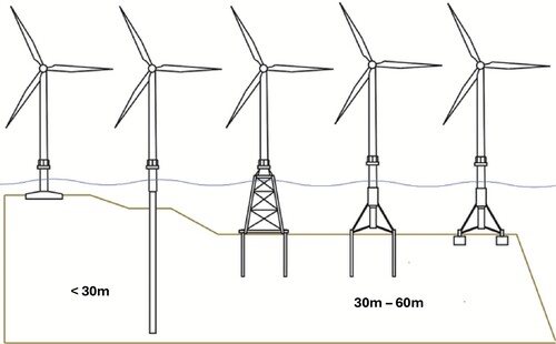
Figure 1 shows different kinds of OWT foundations and their suitable water depth in the offshore renewable energy industry. In this study, an offshore support structure, OC3 (Offshore Code Comparison Collaboration) monopile, was selected to be modelled. It is a tubular pile with a constant section (6 m × 60 mm) for a water depth of 20 m, and it is buried 36 m in multi-layer sandy soil. the details of OC3 can be found in [53].

Figure 1. Different OWT support structures and foundation concepts (Kirkwood, Haigh, and Bhattacharya 2014).

The OWT support structure analysing models can be classified into two groups, i.e. the beam model (1D) and the finite element analysis model (3D FEA). In the 1D beam model, the support structure is discretized into Elastic Euler or Timoshenko beam elements sequence. It is accurate and helpful in computing global structural behaviour, such as deflections and modal frequencies (Tian et al. 2019). However, it is inaccurate in representing a proper structural response for the components at a local scale, for instance, stress concentration effects (Tian et al. 2019). The diversity of the support structure and configuration for the OWT requires FEA (Kuhn 2001). The 3D FEA model is preferred over the 1D beam model due to its high fidelity and the capability to examine detailed stress distributions and accurately capture structural responses within the structure (Wang and Kolios 2017).

Typically, OWT modelling includes a combination of two parts. The first part consists of the turbine blades and nacelle. The second model is the support structure, involving the foundation. In the study by (Petrini et al. 2010), different system model levels have been described, and structural analysis of an OWT is categorised as Meso-level. In this type of modelling, structural responses, such as the stress concentration effect, are represented more accurately compared to Micro-Level (Individual components modelling). In such cases, Meso-level modelling uses a two-dimensional estimation with shell elements. In addition, it is also useful to check the stability of the structure, i.e. the local buckling effect.

As structural analysis science has progressed, optimisation discipline has developed as well. The definition by (Arora, Ge, and Moitra 2012) is that optimisation is an approach to formulating a design case mathematically to find the optimal solution using an algorithmic or semi-automatic method. Optimisation is a challenging stage of every project. Simultaneous consideration of all the disciplines of interest makes the complexity of the problem even more extensive.

Deterministic Optimisation (DO) techniques for support structures have mainly focused on analysing fatigue and ultimate limit states (Gentils, Wang, and Kolios 2017). Design optimisation of structures with probabilistic problem variables and parameters, also known as optimisation under uncertainty, is a vast field of research covering two more extensive areas, i.e. optimisation and probabilistic design. While the DO method gives us an optimal strategy, the presence of uncertainties in material properties or manufacturing tolerances and environmental loads creates a need for more systematic consideration of these uncertainties and probabilistic approaches in a design that copes with the uncertain nature of parameters. Reliability-Based Design Optimisation (RBDO) is a powerful nondeterministic method to reduce the cost of mechanical parts while maintaining a high level of confidence in the design. In this regard, RBDO design has become increasingly popular, affecting various fields (Stieng and Muskulus 2020). However, traditional RBDO methods are computationally expensive. To resolve this, in the other study (Kharmanda, Mohamed, and Lemaire 2002), the author proposed the hybrid method as a solution to decrease the computational cost. This method saves considerable time in the calculation, but the optimisation problem became more complex due to a large number of design variables. Optimum Safety Factor (OSF) was introduced to overcome this problem (Kharmanda et al. 2014); however, the efficiency of these methods has been demonstrated only by considering static cases and some special dynamic ones. This paper introduces a new framework of Reliability-Constrained Optimisation (RCO) to keep the accuracy of results high and the number of variables and computational time as low as possible. Considering the components’ partial safety factors and applying a coupled analysis in the optimisation process are the critical sections of this framework.

Structural Reliability Assessment (SRA) is an applied method to assess the safety levels of OWT structure (Mardfekri and Gardoni 2013). However, a probabilistic description of variability, uncertainty, and sources of error, is often a more natural approach (Mardfekri and Gardoni 2013). Even though several methods have been developed when working on structural reliability analysis concepts of oil & gas platforms, much less work has been done regarding the application of different OWT support structures RCO is one of the complementary approaches and strategies that integrate uncertainty and randomness in the design process both in dynamic and static cases without the complexity of RBDO and the hybrid method (Tsompanakis, Lagaros, and Papadrakakis 2008).

This paper focuses on a framework that uses a parametric model of Finite Element Analysis (FEA) of OWT support structures and integrates this with a Genetic Algorithm (GA) to optimise and reduce the support structure's overall mass while satisfying multiple criteria imposed by design standards. This framework strategy in combining FEA, GA and reliability assessment of the candidate design models allows us to achieve the optimum reliable support structure of OWT considering the target reliability constraints.

2. Methodology

2.1. Deterministic optimisation using a genetic algorithm

As discussed, an OWT support structure is exposed to several levels of uncertainties, which are potential sources of failure. Therefore, optimisation in the early stages of the design process can reduce a significant cost. The result will be a lighter and more robust structure with optimum responses to environmental loads (Muskulus and Schafhirt 2014). Therefore, the first stage before reliability assessment is deterministic optimisation.

This paper uses the GA to find the optimum structure by reducing the mass. The GA procedure uses a selection of mechanisms in both nature and genetics. The algorithm is based on fitness function and genetic representation to optimise a problem. The fitness function is used to assess how well a design point performs compared to the chosen objective function. A design point in GA plays the same role as a chromosome in genes. It contains all system variables. Considering fitness function and genetic representation, the GA continues to modify a group of candidate points and improve the population by frequently using the mutation process (Goldberg and Holland 1988). The lack of restrictions on the form of the objective function is the most significant advantage of genetic algorithms. GA does not require knowledge of the objective function's gradients or higher derivatives, and it has been widely utilised in the optimisation of engineering structures (Al-Sanad et al. 2022; Ferreira et al. 2018; Joshi, Sandhu, and Bansal 2013). GA should solve problems where traditional and other methods are too complex to apply or take too much time (Haupt, Haupt, and Wiley 2004). The number of variables can significantly affect the amount of calculation; thus, the optimum number of variables should be chosen to obtain the optimum solution by minimising the amount of computation.

2.2. Structural Reliability Assessment (SRA)

As discussed, structural reliability assessment is employed to assess the safety levels of the OWT structure. Safety has a direct relation with failure modes. Several time-dependent failure modes of an OWT support structure can directly affect its resistance to applied loads. However, the predominant phenomenon is fatigue damage due to the marine environment and corrosion, which results in the degradation of the components (Price and Figueira 2017) and also because of the amplitude of fatigue loads caused by the mixed responses of wind, wave, and other loads. Consequently, fatigue is a design-driving criterion for an OWT as a welded structure, according to (Dong, Moan, and Gao 2012).

To perform the SRA, a parametric FEA model is built in the ANSYS© at the first step. Then, the various input parameters are given using their corresponding distributions. The developed FEA model is then used to run a series of FEA simulations through the Design of Experiment (DoE) module in the DesignXplorer© of ANSYS.

Choosing a proper sampling method is vital in reliability assessment. The Monte Carlo Sampling (MCS) method (Harrison 2009) is used to calculate the probability of failure (P_f). The MCS approach tries to sample each random variable, X_i to provide a value ${\hat{x}}_i$. Then the limit state function is checked by those x_i values, and if the function is violated, it is noted as a failed structure. (1) $P_f={\displaystyle \frac{n\left(g\right({\hat{x}}_i\le 0)}{N}}$(1) where n is the number of trials in which the limit state function result is more than zero, $g\left({\hat{x}}_i\right)$ is the limit state function, and N is the number of trials.

MCS can calculate the P_f heuristically but cannot transform the limit state function (Lee et al. 2014). MCS randomly simulates the samples, depending on the probability density functions of input variables; therefore, P_f accuracy depends on the iterating sampling size. Latin Hypercube Sampling (LHS) by (Loh 1996) is a variance reduction method that helps the user save time and reduce the number of iterations needed in the MCS method. In this study, LHS with the number of samples equal to $1\times {10}^7$ is selected and applied to all the design constraint cases.

A good design point is typically the outcome of a trade-off between multiple objectives. As a result, optimisation procedures that lead to a single design point during design exploration should be avoided. Enough data on the existing design are required in order to answer ‘What-if’ inquiries regarding how design factors affect product performance. The best judgments can be possibly made based on precise data, even if the design limitations change unexpectedly. DoEs and Response Surfaces (RS) provide all the data needed to develop simulation-driven products. The Response Surface method replaces the original input-output relationship with an approximation function. For the approximation function $\hat{y}$, typically a quadratic polynomial with cross-terms is used in the form: (2) $\hat{y}=C_0+\sum _{i=1}^n{c}_i.x_i+\sum _{i=1}^n\sum _{j=i}^n{c}_{\mathrm{ij}}.x_i.x_j$(2) where $C_0$, $c_i$ and $c_{\mathrm{ij}}$ with i,j = 1, … ,n are the regression coefficients and $x_i$, i = 1, … ,n are the n input variables. Equation (2) is also a regression model. The response domain was derived, and an appropriate response surface model was produced. The response surface model is the interpolation of the values in the multiple dimensions characterised by the DoE. Several types of response surfaces are available in the commercial package of ANSYS DesignXplorer© (Thompson and Thompson 2017), including genetic aggregation, standard response surface full second-order polynomials, kriging algorithms, non-parametric regression, and the sparse grid. In this paper, the standard response surface full second-order polynomials, with manual refinements, are adopted. The second-order model is the most common approximating polynomial model in response surface methods (Bezerra et al. 2008). The Central Composite Design (CCD) presented by (Box and Wilson 1951) is the selected design, as it is the most recommended design for fitting second-order models (Brown and Brown 2012). The goodness of fit metric is also packaged within the response surface module, calculated for the DoE points and can be assessed for verification points to check how accurately the response surface can predict the design points. The predicted and observed chart must be reviewed to show the goodness of fit of data for outputs in all limit state cases. Moreover, the output values should be checked to determine if most points fall on or near the line. The response surface evaluates the values for most of the design points within its range, including the verification points, correctly.

The Six Sigma Analysis (SSA) function of the DesignXplorer© module in ANSYS is employed in this paper for the probabilistic assessment. The Six Sigma Expression was created by Motorola initially (Harry 1987). SSA can also determine the extent to which model uncertainties affect analysis results. To do so, SSA uses several statistical distribution functions to define uncertain parameters. In practice, Six Sigma analysis has been employed for robust design approaches in recent years.

In the ANSYS DesignXplorer© module, the parameters defined in the simulation have been recognised automatically. Design variables or random variables are assigned by the user, and for each of these random variables, a statistical distribution function can be selected.

Finally, the cumulative distribution function (CDF) is used to assess the P_f of the component. The resultant CDF value at any given point shows the probability that the relevant parameter value remains below that point. The equivalent reliability index β is evaluated through appropriate statistical transformation (Melchers and Beck 2018).

2.3. Reliability-Constrained optimisation

A GA-SRA optimisation model is developed in this paper to find the optimal design for OWT by satisfying the criteria specified by design standards, which correspond to a target reliability level. The model combines OWT deterministic optimised candidate design solutions and a simulation model with the Six Sigma reliability assessment. In addition, target reliability constraints will be incorporated within the optimisation process. The general form can be written as: (3) $F_{\mathrm{obj}}=min\left(M_{\mathrm{global}}\right)$(3) Subject to:

1. Implied constraints are given in Section 3.4.2

2. Applied Target Reliability

where $F_{\mathrm{obj}}$ is an objective function that is chosen to minimise $M_{\mathrm{global}}$, the global mass of the support structure. Figure 2 depicts the flowchart of the reliability-constrained design optimisation framework developed in this work.

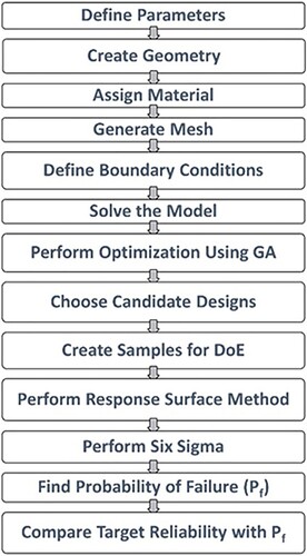
Figure 2. Flowchart of Reliability-Constrained Design optimisation framework.

3. Case study

3.1. Reference model

The reference turbine used in this study is NREL's OWT, developed based on the Senvion 5MW model wind turbines and is considered representative of typical utility-scale land- and sea-based multi-megawatt turbines. The characteristics of this turbine are listed in Table 1. The support structure is a monopile OC3 (J. Jonkman and Musial 2010). The tubular pile has a constant section with 60 mm thickness and 6 m outer diameter. The embedded part of the monopile is 36 m, and the sea depth is 20 m. The transition piece is 10 m above the mean water level. The adopted NREL 5MW and OC3 Monopile geometry implanted in layered sandy soil are illustrated in Figure 3.

Figure 3. Reference model geometry and dimensions.

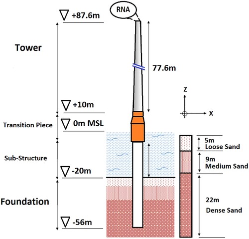
Table 1. NREL 5 MW baseline wind turbine (Jm. Jonkman et al. 2009).

Item	Value
Rating	5 MW
Rotor orientation	Upwind
Control	Variable speed, collective pitch
Drivetrain	High speed, multiple stages, gearbox
Rotor diameter	126 m
Hub height	90 m
Cut-in, rated, cut-out wind speed	3, 11.4, 25 m/s
Cut-in, rated rotor speed	6.9, 12.1 rpm
Rated tip speed	80 m/s
Overhang, shaft tilt, precone	5 m, 5°^, 2.5°
Rotor diameter	126 m
Tower base diameter	6 m
Tower base thickness	0.027 m
Tower top diameter	3.87 m
Tower top thickness	0.19

3.2. Loads and conditions

The site considered in this study is assumed to be located in the North Sea and 8 km away from the city of IJmuiden (Jm. Jonkman et al. 2009).

3.2.1. Applied loads

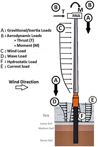
In addition to dead loads, various environmental loads are imposed on the OWTs. IEC 61400-3 (IEC 2019) or DNV-OS-J101 (DNV GL 2014) have suggested a list of loads that should be applied to the structure, and the formulation of these loads is captured from DNV-RP-C205 (Kovacs 2010). The main loads that have been used for our case study are (1) inertia loads; (2) aerodynamic load; (3) wind load applied to the tower; (4) wave load; (5) current load, and (6) hydrostatic loads applied to the support structure.

Due to the mass of the support structure and the RNA mass at the top of the tower, inertia loads can considerably contribute to the buckling and change the modal frequencies of the OWT support structure. Therefore, they should be included in the structural analysis of support structures. In addition, the gravitational loads, system weight and applied loads on the structure impact the modal analysis (Freebury and Musial 2000).

Aerodynamic loads result from the moving parts of the wind turbine and static components. The magnitude of the load is not constant, as it depends directly on wind and air density. The design load values are defined in the WindPACT (Wind Partnership for Advanced Component Technologies) Turbine design study (Malcolm and Hansen 2006). The fatigue design resistance, developed initially by NREL, was calculated by the Damage Equivalent Load (DEL) method. The DEL method was validated in the study by (Freebury and Musial 2000).

The calculated wave load, composed of inertia and a drag term, results from the interaction between the wave and the cylindrical shape of the OWT support structure. Morison's equation can be employed according to DNV-OS-101 (DNV GL 2014) to estimate the amount of the load when the monopile diameter, D, is smaller than 0.2 of wavelength, λ (see Equation (4)). (4) $D\le 0.2\lambda \mathrm{For}\mathrm{Shallow}\mathrm{water}\mathrm{depth}:\lambda =T\sqrt{\mathrm{gh}}$(4) In this study, the water depth, h, is 20 m, and the wave period, T, is 5 sec, so the wavelength is 70 m, which satisfies the above equation. Therefore, Morison's equation is considered the appropriate method to calculate the wave load, see Equation (5). (5) $F_{\mathrm{wave}}\left(z\right)={\displaystyle \frac{1}{4}{\rho }_w.\pi .D^2.C_M.\dot{u}\left(z,t\right)+{\displaystyle \frac{1}{2}{\rho }_{\mathrm{water}}.D.C_D.u\left(z,t\right).\left|u\left(z,t\right)\right|}}$(5) The descriptions and values for Equation (5) are listed in Table 2.

Table 2. Wave load assumption and values.

Item	Description
Monopole Inertia Coefficient, Cm	1.6 (DNV GL 2016)
Monopile Drag Coefficient, CD	1.0 (DNV GL 2016)
Water Density, ${\rho }_{\mathrm{water}}$	1025 Kg/m^3
Horizontal Velocity of Water Particles, $u\left(z,t\right)$	The linear/Airy wave theory (Chakrabarti 2005)
Acceleration of Water Particles, $\dot{u}\left(z,t\right)$	The linear/Airy wave theory (Chakrabarti 2005)

Wind loads on the tower are caused by drag force and are defined by Equation (7). In Equation (7), the power-law profile represents the wind shear as (See Equation (6)): (6) $\overline{V}\left(z\right)={\overline{V}}_r{\left({\displaystyle \frac{z}{z_r}}\right)}^{\alpha }$(6) where α is the roughness coefficient, and its value is taken as 0.115 considering the offshore condition (J. Jonkman and Musial 2010). The reference wind speed ${\overline{V}}_r$ is measured at the nacelle reference height, $z_r$. Finally, wind loads can be calculated by: (7) $F_{\mathrm{tower}}\left(z\right)={\displaystyle \frac{1}{2}{\rho }_a{C}_{D,T}D\left(z\right)V_r^2\left(z\right)}$(7) The Drag Coefficient, $C_{D,T}$ is 1.0 (Chehouri et al. 2015), D(z) is the external diameter of the tower segment at the height of z, and the outer diameter of the tower narrows at the height of $z$. 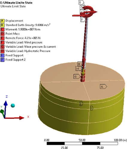Figure 4 shows schematic OWT support structure with all applied loads.

Figure 4. Applied loads on OWT support structure.

The outer surface of the monopile is subjected to hydrostatic pressure when it is submerged in water. This is a constant normal load that increases linearly with water depth. Therefore, the hydrostatic force, F_h, can be calculated using the gravitational constant, g, and water depth, h, (see Equation (8)): (8) $F_h={\rho }_w\mathrm{gh}$(8)

3.2.2. Design load cases

Several load cases that cover all conditions of OWTs design are defined in (Kovacs 2010), with (IEC 2019) as a reference. As suggested by (Schaumann et al. 2011), two structurally prominent load cases have been considered. The ultimate load case (ULC) corresponds to extreme environmental conditions based on a 50-year return period.

Previous studies revealed that wind load is the dominant load acting on the 5MW NREL compared to wave load (Gentils, Wang, and Kolios 2017b; Muskulus and Schafhirt 2014). Thus, under the 50-years Extreme Wind Model (EWM) with the 50-years Reduced Wave Height (RWH) and Extreme Current Model (ECM), defined as the Design Load Case (DLC) 6.1b and 2.1 for IEC [41] and GL [8] standards, the most critical ULS load case is often considered to correspond to the parked wind turbine. According to standards (IEC 2019), the safety factors for the design loads are 1.1 and 1.35 for gravitational and environmental loads, respectively.

Fatigue load case (FLC) is another load case caused by variation in operation and cyclic loads. FLC is an essential source of cyclic loading during the OWT lifetime. In the current case study, a popular load scenario for FLS is an operating state under the Normal Turbulence Model (NTM) and the Normal Sea State (NSS), where wave height and cross zero periods were calculated using the site's joint probability function, assuming no current. It was thought to represent the entire fatigue state because it covers more than 80% of the fatigue damage. It corresponded to the DLC 1.2 from the IEC standard [7,35]. It was assumed to represent the entire fatigue state because it covers more than 80% of the fatigue damage. According to (IEC 2005), the safety factor for this load case is equal to 1.0. Tables 3 and 4 summarise the load cases and aerodynamic loads applied to the model, respectively.

Table 3. Wind turbine aerodynamic loads, (Jm. Jonkman et al. 2009).

Load Case	Tilting moment (kN.m)	Thrust force (kN)
ULC	38567	781
FLC	3687	197

Table 4. Design load cases, (IEC 2005).

Load case	Wind	Wave	Load safety factor
Ultimate: DLC 6.1b/2.1	EWM: $V_{g50}$	RWH: $1.32\times H_{s50},T_{s50}$	– 1.0
(Parked)		ECM: $V_{c,\mathrm{ex}}$
Fatigue: DLC 6.1b/2.1	NTM: $V_{\mathrm{ave}}$	NSS: $H_{\mathrm{ave}},T_{\mathrm{ave}}$	Normal N 1.1/1.35
(Parked)		No Current

3.3. Parametric FEA model

A parametric finite element model is performed using the ANSYS workbench. The modelling phase started by defining the parameters, for instance, geometry data, material properties and structure thickness.

3.3.1. Geometry and applied loads

A 3D model consisting of five parts was created using the previous section's geometrical parameters, i.e. soil, tower, grout, monopile, and transition piece. Respectively, the monopile and tower parts were sectioned into 10 and 15 pieces. The diameter of soil was considered 20 times the diameter of the monopile support structure. This is large enough to prevent pile-soil behaviour from being influenced by boundary effects. Figure 5 shows the reference model used in this case study. As the reference documents recommend, this model was created with precise tower dimensions, transition piece, grout, and monopile [34]. Wind, wave, and current load profile data have been calculated and applied as variable loads on the outer area of the structure. Thrust force is located at the tower's designated point at the top. The moment is applied to the whole structure. Gravitational load is located downward on the centre of mass of the support structure. Details are illustrated in Figure 6.

Figure 5. NREL 5MW wind turbine and OC3 platform geometry.

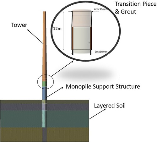
Figure 6. Isometric view of geometry and applied loads.

3.3.2. Material

According to (DNV GL 2016), the support structure's primary material is S355 Steel. The grout material is Ducorit D4. Sand properties are defined by using the Drucker-Prager model (Lacher 2013). According to this model, the soil yield strength can be defined in terms of cohesion value and friction angle as in Equation (9): (9) ${\sigma }_{y,s}={\displaystyle \frac{6c\cos \left(\varphi \right)}{\sqrt{3}\left(3-\sin \left(\varphi \right)\right)}}$(9) where ϕ is the friction angle, c is the cohesion value of which value is given in Ref. (Ma and Chen 2021). Thus, the friction between pile and soil can be driven by Equation (10) (Jung et al. 2015): (10) $C_f=\tan \left({\displaystyle \frac{2}{3}\varphi }\right)$(10) Regarding the above equations and soil properties adopted from (Jung et al. 2015), the soil characteristics and other material used in this study (DNV GL 2016; Theotokoglou and Papaefthimiou 2017) are summarised in Tables 5 and 6. In addition, the contacts between the soil and the monopile are defined in ANSYS, considering the friction coefficients.

Table 5. Sand properties in different levels (Jung et al. 2015).

Sand Type	Young’s Modulus (MPa)	The angle of friction (deg)	Friction coefficient	Yield stress (kPa)
Loose	30	33	0.40	59.2
Medium	50	35	0.43	58.5
Dense	80	38.5	0.48	57

Table 6. Support structure material properties.

Item	Steel	Grout
Young Modulus, E (GPa)	210	70
Density (kg/m^3)	8500	2740
Poisson’s ratio	0.38	0.19
Tensile Strength (MPa)	–	10
Yield Strength (MPa)	355	–

3.3.3. Meshing

Mesh generation is an essential step in FEA simulation since it is susceptible to the result's accuracy. In this work, the shell element type, Shell281, was used for the thin-wall structures such as tower and monopile. Shell281 characteristics are suitable for considerable strain nonlinearity and large rotation applications (Thompson and Thompson 2017); therefore, it is appropriate for this study. The grouting part is meshed by the element SOLID186 to obtain accurate bending stress considering the friction. Finally, SOLID185 was used for the soil part.

Mesh convergence is performed to obtain an accurate result. The process starts with applying 100 kN Force on top of the tower. The application of 100 kN Force is a test force on top of the structure to optimise the mesh in the x-direction. Because the mesh quality check is essential, it could be any value or any type of load in any direction, but a single force is preferred to reduce the calculation run time. The calculated maximum Von Mises value converges after using a mesh type with an element size of 1 m (37,356 elements) refinements by comparing the result values and the differences. Figure 7 illustrates the final optimum mesh, and Table 7 presents the optimum number of elements. Comparing the values and the differences, Mesh #3 is selected in order to proceed with the analysis.

Figure 7. Final generated mesh.

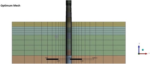
Table 7. Mesh sensitivity.

Description	Element size of Steel part	Number of Elements	Max Von Mises (MPa)
Mesh #1	4 m	1780	25.4
Mesh #2	2 m	7584	23.1
Mesh #3	1 m	37356	23.0
Mesh #4	0.5 m	235180	23.0

3.3.4. Boundary condition

Boundary conditions are applied to the geometry, as the bottom of the soil model is fixed in all directions. Side boundaries of the soil are fixed against lateral translation. Contact between soil and monopile is set according to the frictional coefficients, and other contacts are assumed as bonded. On top of the tower, wind turbine rotor aerodynamic loads are applied. Other loads (such as wave, current, wind loads, and hydrostatic loads) are applied using pressure formulations, which allow these loads to automatically update with the updated diameters of the support structure during the optimisation process in a more accurate representation. Hydrostatic loads surround the submerged components. The RNA is a concentrated mass applied to the tower top via a multi-point constraint.

3.3.5. Fea model validation

The geometry is validated by comparing the results from the current model and the reference model. A case study defined in (Damiani et al. 2013), in which a 2MN rotor thrust load has been applied to the top of the tower. Considering the weight of the nacelle and blades, the results show good agreement with the reference model. The values are presented in Table 8, which confirms the validation of the present model.

Table 8. Deformation in the reference model and current model.

Load case	Deformation
Mass/Thrust	Current model	Reference model	%Diff
2MN + Weight	1.676 m	1.644 m	+1.94%

3.4. Deterministic structural optimisation analysis

As this study aims at developing an integrated optimisation methodology, the minimum global mass of the support structure is chosen as the objective function. The mass reduction in an OWT support structure is to achieve cost reduction goals. Partial safety factors (PSFs) are applied according to DNV standards (DNV GL 2016).

3.4.1. Design variables

According to (Kallehave et al. 2015; Muskulus and Schafhirt 2014), thickness and diameter dimensions are two types of variables that significantly influence structural response and are individually designed driven by different criteria. Defining several sections on the tower and monopile caused an increase in the number of variables. This issue can be a challenge in the simulation process and calculation time. A reduction technique has been introduced by (Ashuri 2012), which uses a linear interpolation between the top and bottom ends. This strategy has been adopted and applied to the tower, foundation and monopile. As a result, the number of variables decreased from 30 to 13 in the final process. It should be noted that the diameter of the foundation section stays constant all along the length due to installation limitations. 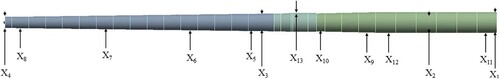So, design variables for a design point j can be stated in Equation 11 as a vector of variables inspired by the chromosome formulation: (11) $X_j=[x_1{x}_2{x}_3\dots x_n{]}^T\mathrm{with}n=13$(11) where x₁ and x₂ are the diameters at the base and top of the monopile; x₃ and x₄ are the diameters at the bottom and top of the tower; x₅, x₆, x₇ and x₈ are the thickness at the base and top of the tower; x₉ and x₁₀ are the thickness at the bottom and top of the sub-structure and x_11; x₁₂ are the thickness along the foundation; x₁₃ is the thickness of the transition piece. In Figure 8, the position of all variables is presented. The list of variables with their upper and lower bounds is available in Table 11.

Figure 8. Design variables of OWT support structure.

3.4.2. Design constraints and criteria

Choice of criteria is paramount for the reliability of optimisation solutions. A wrong choice or lack of proper criteria could lead to unexpected structural failure during experimental tests or structure lifetime. This paper defined seven structural constraints based on modal, stress, deformation, bucking, and fatigue requirements. Geometrical constraints on the design variables were also considered and are described below. It's worth noting that the turbine's foundation and tower are both composed of steel. If the turbine's tower is composed of composite material, it should be addressed independently from the monopile base.

3.4.2.1. Resonance constraint

As seen in Figure 9, OWTs are dynamically loaded structures, with loads coming from the wind, waves, and rotor excitations. The fundamental frequency f₀ (the first tower bending frequency) and the dynamic interaction with the external loads have a strong influence on the structure's response. This occurs when f₀ is higher than the rotor's rotational frequency, f_1P, which is caused by rotor imbalances, but lower than the blade-passing frequency, f_3P, which is caused mainly by aerodynamic impulse loads when the blades pass the tower [46]. To avoid resonance phenomena, first natural frequency f_1st should be sufficiently separated from the turning rotor induced frequencies f_1P and blade-passing frequency f_3P. The structure’s natural frequency should be between f_1P and f_3P (Gentils, Wang, and Kolios 2017b).

Figure 9. Illustration of typical excitation ranges of a modern OWT (Kallehave et al. 2015).

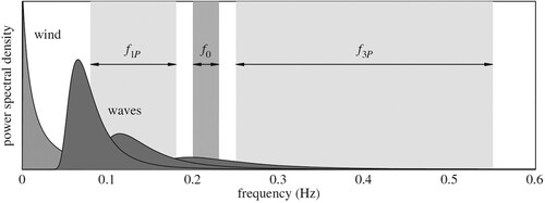
According to (DNV GL 2010, 2011), the first natural frequency should avoid rotor induced frequencies with a tolerance of ±5%: (12) $f_{1P\pm 5\text{\%}}\le f_{1\mathrm{st}\pm 5\text{\%}}\le f_{3P\pm 5\text{\%}}$(12) The cut-in and rated rotor speed of the NREL 5MW are 6.9 and 12.1 rpm, respectively. f₀ would be roughly 0.20–0.23 Hz for a 6–8 MW offshore wind turbine on a monopile constructed for the soft – stiff frequency range [46]. Therefore, resonance constraints are: (13) $0.212\mathrm{Hz}\le f_{1\mathrm{st}}\le 0.328\mathrm{Hz}$(13)

3.4.2.2. Stress constraints

In the Ultimate Limit State (ULS), the maximum stress of the support structure σ_VM,ax (Von Mises) should stand below the allowable stress limits σ_VM,allow. The following inequality expresses this. (14) ${\sigma }_{\mathrm{VM},\max }\le {\sigma }_{\mathrm{VM},\mathrm{allow}}$(14) The allowable stress value σ_VM,allow is derived from Equation (15): (15) ${\sigma }_{\mathrm{VM},\max }={\displaystyle \frac{{\sigma }_{y,\mathrm{Steel}}}{{\gamma }_m.{\gamma }_f}}$(15) where σ_y,steel is the steel component's yield strength; γ_m and γ_f are the PSFs for material and consequence of failure, respectively. The yield strength for S355 steel is 355 MPa is adopted from (Arshad and O’Kelly 2013). Furthermore, the PSFs for material γ_m and failure γ_f are 1.1 and 1.0 (IEC 2005), respectively. Thus, the allowable stress σ_VM,llow is 322.7 MPa.

3.4.2.3. Deformation constraints

The stability of the monopile foundation is a vital factor in ULS. Therefore, rotation and deflection constraints have been defined to ensure that pile-head deflection d_pile and seabed rotation θ_seabed values are less than allowable values. These constraints could be expressed by: (16) $d_{\mathrm{pile}}\le d_{\mathrm{allow}}$(16) (17) ${\theta }_{\mathrm{seabed}}\le {\theta }_{\mathrm{allow}}-{\theta }_{\mathrm{inc}}$(17) where ${\theta }_{\mathrm{inc}}$ is the installation uncertainty and was chosen analytically here at 0.1°. According to DNV standard (DNV GL 2016), the values of $d_{\mathrm{allow}}$ and ${\theta }_{\mathrm{allow}}$ were fixed at 0.1 m and 0.5°, respectively. The material safety factor γ_m of 1.0 was applied for the soil strength in this section (DNV GL 2016).

3.4.2.4. Buckling constraints

The risk of instability due to buckling is not negligible in a monopile's design and optimisation process due to the slenderness of the tower and sizeable weighted Rotor – nacelle assembly (RNA) at the top. The results of the ULS static analysis are used as pre-stress loads. To avoid this type of failure in ULS mode, the load multiplier L, the ratio of the critical load to the current applied load, should be larger than the allowable load multiplier L_m,allow. ANSYS software determines the critical load for buckling analysis by solving an eigenvalue problem. The process is fundamentally based on comparing the structure’s stiffness to its susceptibility to buckle under a given load. If the buckling load multiplier is negative, the model will buckle when the applied loads are reversed (and scaled by the multiplier). For example, A buckling multiplier of – 0.75 implies that the part will buckle with a 750 Pa compression load if a pressure of 1000 Pa is applied to the model, but this puts it in tension. According to (DNV GL 2010), L_m,llow value of 1.4 has been chosen. This constraint could be expressed by: (18) $L_m\ge L_{m,\mathrm{allow}}$(18)

3.4.2.5. Fatigue constraints

As discussed earlier, fatigue is the main governing factor for the OWT support structure design process. Therefore, the design life-number of cycles N_life- could be assessed based on rated rotor speed n_rated (12.1 rpm) and availability η_a (98.5%) of the chosen installation area (Kuhn 2001). Thus, considering a lifetime requirement of 20 years (DNV GL 1987; Kovacs 2010), the number of cycles to be expected is 1.25 × 10⁸: Using the design life number, N_life, and S-N curve, the design fatigue stress range, σ_f,Design can be derived. In this case study, global fatigue stress is considered. (19) $N_{\mathrm{life}}={\eta }_a\times n_{\mathrm{rated}}\times \left(60\min \times 24\mathrm{hr}\times 365\mathrm{day}\times 20\mathrm{years}\right)$(19) An appropriate S-N curve of slope m = 4 and loga = 13.93 was provided by (LaNier 2005). The maximum fatigue stress range σ_f,max in the OWT support structure subjected to the fatigue loads is calculated from the FEA simulations. It should be noted that the stress used in the fatigue analysis is the von-Mises stress. The minimum fatigue safety ratio f_sr,in could then be derived from the design stress σ_design over the maximum fatigue stress σ_f,max in the structure. This safety ratio should stay above the allowable fatigue safety ratio f_allow, which is equal to one, times the material PSF γ_m. Fatigue constraint can be written as: (20) $f_{\mathrm{allow}}\ge f_{\mathrm{sr},\min }$(20) The PSF of material for the Fatigue Limit State is 1.15 (DNV GL 1987, 2016); therefore, f_allow is equal to 1.15.

3.4.3. Genetic algorithm

As the FE Model is parametric, the parameters involved in the optimisation process in the multi-objective GA procedure can be easily chosen and updated. The initial samples are created and individually solved by the respective module when the optimisation process is run. After all the initial samples have been solved, the specified optimisation algorithm is automatically run. The optimisation module suggests two candidates that meet the requirements at the end of the process. A GA is divided into five parts: initialisation, fitness assignment, selection, crossover, and mutation [21]. The number of initial samples should be at least ten times the number of design variables. This value was increased by 200 points in this study to improve the chances of finding a better solution (Haupt, Haupt, and Wiley 2004). Convergence speed is affected by the number of samples per iteration.

In this study, an empirical value of 50 is chosen. The output parameters’ maximum spread, mean, and standard variation calculate the convergence criterion. When the criteria value reached 1.5 per cent, optimisation was assumed to have converged, implying a homogeneous population. The maximum number of iterations is the blocking criteria of the algorithm. Cross over probability is a value between 0–1. A low value encourages the use of available design points (parents), whereas a high value encourages the exploration of new designs through offspring generation. A crossover probability of 0.90 (Haupt, Haupt, and Wiley 2004) is used in this study. The probability of mutation must be between 0 and 1. A higher value increases the algorithm's randomness until it becomes a simple random search for a value of one. This study uses a typical mutation probability of 0.01 [25]. The ‘performance’ of a genetic algorithm depends highly on the method of encoding candidate solutions into chromosomes and ‘the particular criterion for success,’ or the fitness function measuring. The probability of crossover, the probability of mutation, the size of the population, and the number of iterations are all critical details. After a few trials runs, these values can be adjusted based on the algorithm's performance. In Table 9, the main characteristics and settings of the GA have been provided.

Table 9. Settings of GA.

Parameter name	Value
Number of initial samples	200
Number of samples per iteration	50
Convergence stability criteria	1.5%
Maximum number of iterations	25
Crossover probability	0.9
Mutation probability	0.01

After using GA settings and applying them to the parametric FEA model, the requested Candidate Points number under the properties table pane displays up. The quantity of gold stars or red crosses next to each objective-driven parameter indicates how well it matches the specified objective. For instance, three red crosses are the worst, and three gold stars represent the best. The user can also add and edit its candidate points, view values of candidate point expressions, and calculate the percentage of variance for each parameter for which a goal has been established in the table panel. Two Candidate Points have been chosen to investigate in this case study. These models were used to assess their reliability with described limit states.

3.5. Six sigma reliability assessment

Selecting appropriate stochastic variables and assigning appropriate statistical distributions are vital for the methodical consideration of uncertainty through reliability analysis. Even though the stochastic data are characterised in this application by normal distributions, the framework can accommodate any statistical distribution variables through appropriate consideration. In this section, ANSYS converted the input parameters from the DoE function and produced sets of stochastic variables based on the defined statistical distribution. A series of deterministic FEA simulations were performed, and then the results were exported to the Response Surface Module to map the response with those design points. The Six Sigma module uses these results to assess the system's reliability. The corresponding reliability index β is evaluated by appropriate statistical transformation (Melchers and Beck 2018). Table 10 shows the mean values and standard deviation of the stochastic variables.

Table 10. Design Variables (Jm. Jonkman et al. 2009).

Stochastic variables	Ultimate load case		Fatigue load case		CoV	Distribution type
	Mean value	Standard deviation	Mean value	Standard deviation
Wind Thrust (kN)	781	78.1	197	19.7	0.1	Normal
Torsional Moment (kN.m)	38,567	3856.7	3686	368.6	0.1	Normal
Tilting Moment (kN.m)	7876	787.6	3483	348.3	0.1	Normal
Steel Young’s Modulus (GPa)	210	21	210	21	0.1	Normal
RNA Mass (Tonne)	350	35	350	35	0.1	Normal

When structural reliability analysis is carried out, suitable safety levels must be selected considering failure, applicable rules, access for inspection, and repair; this safety level is called the target safety level. According to DNV guidelines (DNV GL 2011), designs’ target annual failure probability is 1E-4.

It should be noted that, in DO, the methodology contains specified reliability as the PSF is included. Thus, these safety factors must be eliminated in the reliability assessment.

4. Results and discussion

4.1. FEA Deterministic optimisation analysis results

The results from FEA Deterministic Optimisation (Candidate Design 1) are presented in Figure 10(a) for maximum Von Mises equivalent stress, Figure 10(b) for buckling, Figures 10(c) and (d) for total deformation and mudline displacement in the ULC, Figure 10(e) for modal analysis, and Figure 10(f) for safety factor in fatigue load condition.

Figure 10. FEA DO analysis results for design candidate 1, (a) Von Mises equivalent stress, (b) Buckling deformation, (c) mudline displacement, (d) Total deformation, (e) 1st mode frequency and displacement, (f) Fatigue minimum safety factor.

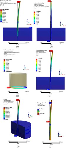
The global maximum equivalent stress equals 287 MPa, 11% less than the allowable stress of 323 MPa. The maximum deformation of the whole support structure is 2.94 m, which shows the considerable deflection experienced by the structure; however, considering the foundation and soil deformation of 0.077 m which is 23% lower than the allowable 0.1 m. Also, 0.351 degrees rotation at the mudline is observed, which is 12.2% less than the permissible value of 0.4. This implies the current support structure design is unlikely to experience large deflections. The buckling load multiplier in this result is 1.68; the limit value for this section is 1.4. This difference shows that the present support structure design is safe under maximum buckling loads.

Modal analysis gives the resonance evaluation and dynamic properties of the structure. The frequency of the first mode is 0.231 Hz which is acceptable for our modal frequency limitation. However, as the frequency is one of the important drivers in the OWT design process and considering that the thicknesses of some parts and the diameter have decreased for the optimisation process, a reliability assessment must be carried out to check the structural reliability. Furthermore, in association with stress distribution, critical fatigue failure location is keen to appear at the top of the tower. Therefore, the minimum safety factor occurs on top of the tower and is equal to 1.194, which is 5.1% higher than the minimum allowable value of 1.15; as a result, the current design can survive its design lifetime under fatigue-inducing loads.

The values of the design parameters obtained from DO are summarised in Table 11. The OWT is optimised only for explicit and implicit constraints in Section 3.4.2 without implementing the reliability constraints in the deterministic analysis. These results show that the 5MW NREL OWT support structure mass can be reduced by 19.7% (Design 1) and 19.95% (Design 2).

Table 11. Deterministic optimisation results.

	Variable	Name	Unit	Lower bound	Initial design	Optimised design (Candidate 1)	Optimised design (Candidate 2)	Upper bound
Design Variables	Monopile base diameter	X1	[m]	5	6	6.10	6.10	7
	Monopile top diameter	X2	[m]	5	6	5.34	5.28	7
	Tower base diameter	X3	[m]	5	6	5.28	5.28	7
	Tower top diameter	X4	[m]	3	3.87	3.28	3.38	4.5
	Tower base thickness	X5	[mm]	20	27	30	31	40
	Tower Int1 thickness	X6	[mm]	20	25	26	26	40
	Tower Int2 thickness	X7	[mm]	15	22	21	22	35
	Tower top thickness	X8	[mm]	10	19	17	17	30
	Monopile substructure base thickness	X9	[mm]	45	60	46	45	70
	Monopile substructure top thickness	X10	[mm]	45	60	45	45	70
	Monopile foundation base thickness	X11	[mm]	40	60	45	46	70
	Monopile foundation top thickness	X12	[mm]	45	60	46	45	70
	Transition piece thickness	X13	[mm]	25	30	33.54	33.43	40
Objective function Constraints	1st Natural frequency		[Hz]	0.21	0.285	0.231	0.223	0.328
	Maximum equivalent Stress (Von Mises)		[MPa]	–	185	287	299	323
	Pile head deflection		[m]	–	0.057	0.079	0.08	0.1
	Pile head rotation		[°]	–	0.26	0.34	0.34	0.4
	Buckling load multiplier		–	1.4	2.35	1.68	1.56	–
	Minimum fatigue safety ratio		–	1.15	1.54	1.19	1.21	–
Mass Saving	Support Structure mass		[Tonnes]	–	924.5	741.4 (−19.7%)	739.1 (−19.95%)	–

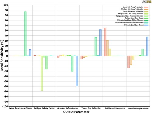
Figure 11 reveals how sensitive the independent input variables are to the whole support diameter. This analysis helps designers examine which variable contributes the most to changes in the structural response and reliability performance. As expected, thrust and tilting moment drastically impact maximum equivalent stress in the ULC. In the FLC, both tilting and torsional moments, and thrust load in operational conditions, influence the margin of safety calculation. Material properties such as soil Young’s Modulus depend on the deformation and displacement of the structure and pile in the mudline, in addition to thrust and moments. It is evident that these material properties are the modal analysis's main parameters, as can be seen in the 1st Natural Frequency section.

Figure 11. Global sensitivity analysis.

4.2. Reliability-constrained analysis results

A new framework for optimising an OWT support structure by assessing the reliability of complex support structures in parallel, was developed in the previous sections. The reliability-constrained analysis results are shown in Table 12. The framework was applied to the NREL 5 MW OWT monopile structure, accounting for several stochastic input variables and multiple limit states. The case study is used to validate the framework's main components. The failure probability value had been extracted from the cumulative density function (CDF) and probability density function (PDF) of the design parameters. Figure 12 a-e presented the CDF and PDF of design constraints of candidate design one.

Figure 12. Cumulative density function and probability density function of design candidate 1 for (a) Fatigue minimum safety factor; (b) Equivalent stress maximum; (c) First natural frequency; (d) Buckling load multiplier; (e) Total deflection.

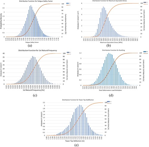
Table 12. Reliability-Constrained analysis result.

Reliability-Constrained Candidate Designs Comparison
	Initial Design		Candidate Design 1		Candidate Design 2
	Pf	β	Pf	β	Pf	β
Ultimate Limit State
Max Stress Capacity	1.3E-06	4.71	3.0E-5	4.01	3.5E-5	3.99
Buckling Capacity	≈0	7.01	4.1E-5	3.94	5.3E-5	3.88
Maximum Deflection	≈0	7.61	6.0E-8	5.28	9.0E-8	5.21
Resonance Capacity	2.1E-08	5.48	5.9E-5	3.85	2.1E-4	3.53
Fatigue Limit State
Min Safety Factor	8.0E-06	4.32	6.1E-05	3.84	7.9E-5	3.81

In this framework, to accept or reject the suggested design, the reliability constraints of the target level of 1E-4 (or Reliability Index of 3.8) should be considered and compared with the reference and two final proposed models from GA optimisation ANSYS. The comparisons of design parameters obtained from different models indicate that the P_f in the optimised model decreased significantly in the buckling and resonance capacities due to the reduction in tower and monopile diameter. As shown in the results, the reliability assessment performed on the structure revealed that candidate design number one, for the modelling of the stochastic variables considered, meets the recommended reliability assessment criteria, as the reliability indices for all of the design constraints considered are within the design thresholds. Nevertheless, candidate design number two is rejected because it has less probability of failure than the target reliability level in resonance capacity, despite the fact that the deterministic optimisation passes both designs.

5. Conclusions

In this study, an RCO framework for OWT support structures was developed. A parametric FEA model of OWT monopile support structures took stochastic environmental loads and material properties into account. The parametric FEA model was optimised with the GA method and then combined with the response surface and Six Sigma functions to evaluate the reliability of optimised models. ANSYS, the FEA software, was manually set to give us the final two candidate support structure designs. The reliability index and probability of failure of optimised OWT structures are calculated and compared with the target reliability defined according to regulations. Candidate design one was chosen as the ultimate optimised model after considering the target reliability index constraint. In general, the following conclusions can also be drawn from this study:

• Good agreement is observed when comparing the deflection of the tower top section of the reference OWT and the ANSYS models, which confirms the validity of the initial FEA model.

• The whole mass of the structure is reduced by 19.7% after the optimisation process.

• A practical response surface approach evaluates the failure function at sampling points. In addition, a modified Monte Carlo simulation with a Latin Hypercube reduction method technique is applied to assess the failure probability.

• The necessity for Reliability-Constrained Optimisation for a large OWT in harsh environmental conditions is evident. This optimisation framework has been proved to be the acceptable reliability index limit of the suggested optimum design model (Candidate Design 1) achieved from deterministic optimisation. Furthermore, the results obtained fall within the recommended design constraints for all limit states.

• This study shows that not all suggested deterministic optimised design candidates fulfil structural reliability criteria. For instance, the reliability index in resonance capacity in Candidate two exceeds the allowable value, although the design achieves all limit state function criteria.

Disclosure statement

No potential conflict of interest was reported by the author(s).

References

- Al-Sanad, Shaikha, Jafarali Parol, Lin Wang, and Athanasios Kolios. 2022. “Structural Optimisation Framework for Onshore Wind Turbine Towers Considering Multiple Design Constraints.” International Journal of Sustainable Energy 41 (5) Taylor & Francis: 469–491. https://doi.org/10.1080/14786451.2021.1953495.
- Arora, Sanjeev, Rong Ge, and Ankur Moitra. 2012. “Learning Topic Models - Going beyond SVD.” Proceedings - Annual IEEE Symposium on Foundations of Computer Science, FOCS. IEEE, 1–10. https://doi.org/10.1109/FOCS.2012.49.
- Arshad, Muhammad, and Brendan C. O’Kelly. 2013. Offshore Wind-Turbine Structures: A Review 166:139–152.
- Ashuri, T. 2012. Beyond Classical Upscaling : Integrated Aeroservoelastic Design and Optimization of Large Offshore Wind Turbines.
- Bezerra, Marcos Almeida, Ricardo Erthal Santelli, Eliane Padua Oliveira, Leonardo Silveira Villar, and Luciane Amélia Escaleira. 2008. “Response Surface Methodology (RSM) as a Tool for Optimization in Analytical Chemistry.” Talanta 76 (5): 965–977. https://doi.org/10.1016/j.talanta.2008.05.019.
- Box, G.E.P., and K.B. Wilson. 1951. “On the Experimental Attainment of Optimum Conditions.” Journal of the Royal Statistical Society: Series B (Methodological) 13:1–38. https://doi.org/10.1111/j.2517-6161.1951.tb00067.x.
- Brown, J.N., and R.C. Brown. 2012. “Process Optimization of an Auger Pyrolyzer with Heat Carrier Using Response Surface Methodology.” Bioresource Technology 103 (1) Elsevier Ltd: 405–414. https://doi.org/10.1016/j.biortech.2011.09.117.
- Burton, Tony, Nick Jenkins, David Sharpe, and Ervin Bossanyi. 2011. Wind Energy Handbook. 2nd ed. https://doi.org/10.1002/9781119992714.
- Chakrabarti, Subrata. 2005. Hand Book of Offshore Engineering (2-volume set). Elsevier.
- Chehouri, Adam, Rafic Younes, Adrian Ilinca, and Jean Perron. 2015. “Review of Performance Optimization Techniques Applied to Wind Turbines.” Applied Energy 142 (Elsevier Ltd): 361–388. https://doi.org/10.1016/j.apenergy.2014.12.043.
- Clauss, G.F., and L. Birk. 1997. “Hydrodynamic Shape Optimization of Large Offshore Structures.” Proceedings of the Conference on Optimization in Industry 1187 (96): 195–200.
- Collette, Yann, and Patrick Siarry. 2003. Multiobjective Optimization: Principles and Case Studies (1st ed.). Paris: Springer Science & Business Media.
- Damiani, Rick R., Huimin Song, Amy N. Robertson, and Jason M. Jonkman. 2013. “Assessing the Importance of Nonlinearities in the Development of a Substructure Model for the Wind Turbine CAE Tool Fast.” Proceedings of the International Conference on Offshore Mechanics and Arctic Engineering - OMAE 8 (March). https://doi.org/10.1115/OMAE2013-11434.
- DNV GL. 1987. “RP-C203: Fatigue Design of Offshore Structures.” Welding International 1 (12): 1155–1161. https://doi.org/10.1080/09507118709452166.
- DNV GL. 2010. “DNV-RP-C201: Buckling Strength of Plated Structures.” (October): 33.
- DNV GL. 2011. “OS-C101: Design of Offshore Steel Structures, General - LRFD Method.” Det Norske Veritas 2018 Ed (April): 49.
- DNV GL. 2014. “DNV-OS-J101 Design of Offshore Wind Turbine Structures.” (May): 212–214.
- DNV GL. 2016. “DNV-ST-0126: Support Structures for Wind Turbines.” (July).
- Dong, Wenbin, Torgeir Moan, and Zhen Gao. 2012. “Fatigue Reliability Analysis of the Jacket Support Structure for Offshore Wind Turbine Considering the Effect of Corrosion and Inspection.” Reliability Engineering and System Safety 106 (Elsevier): 11–27. https://doi.org/10.1016/j.ress.2012.06.011.
- Ferreira, Ana C M, Senhorinha F C F Teixeira, Rui G Silva, and Ângela M Silva. 2018. “Thermal-Economic Optimisation of a CHP Gas Turbine System by Applying a Fit-Problem Genetic Algorithm.” International Journal of Sustainable Energy 37 (4) Taylor & Francis: 354–377. https://doi.org/10.1080/14786451.2016.1270285.
- Freebury, G., and W. Musial. 2000. “Determining Equivalent Damage Loading for Full-scale Wind Turbine Blade Fatigue Tests.” 2000 ASME Wind Energy Symposium (c): 287–297. https://doi.org/10.2514/6.2000-50.
- Gentils, T., L. Wang, and A. Kolios. 2017b. “Integrated Structural Optimisation of Offshore Wind Turbine Support Structures Based on Finite Element Analysis and Genetic Algorithm.” Applied Energy 199 (August): 187–204. https://doi.org/10.1016/j.apenergy.2017.05.009.
- Gentils, T., L. Wang, and A. Kolios. 2017. “Integrated Structural Optimisation of Offshore Wind Turbine Support Structures Based on Finite Element Analysis and Genetic Algorithm.” Applied Energy 199 (August): 187–204. https://doi.org/10.1016/j.apenergy.2017.05.009.
- Goldberg, David E., and John H. Holland. 1988. Genetic Algorithms and Machine Learning. The Netherlands: Kluwer Academic, 95–99.
- Harrison, Robert L. 2009. “Introduction to Monte Carlo Simulation.” AIP Conference Proceedings 1204 (IEEE): 17–21. https://doi.org/10.1063/1.3295638.
- Harry, Mike J. 1987. “The Nature of Six Sigma.Pdf.”
- Haupt, Randy L, Sue Ellen Haupt, and A. John Wiley. 2004. Algorithms Second Edition.
- IEC. 2005. “IEC 61400-1.” IEC 61400–01 (2): 88. https://doi.org/10.4172/2155-9600.1000405.
- IEC. 2019. “IEC 61400-3-1.” IEC, 1–11.
- Ivanhoe, R.O., L. Wang, and A. Kolios. 2020. “Generic Framework for Reliability Assessment of Offshore Wind Turbine Jacket Support Structures under Stochastic and Time Dependent Variables.” Ocean Engineering 216 (August 2018) Elsevier Ltd: 107691. https://doi.org/10.1016/j.oceaneng.2020.107691.
- Jonkman, Jm, S. Butterfield, W. Musial, and G. Scott. 2009. “Definition of a 5-MW Reference Wind Turbine for Offshore System Development.” NREL (February): 1–75. https://doi.org/10.1002/ajmg.10175.
- Jonkman, J., and W. Musial. 2010. “Offshore Code Comparison Collaboration (OC3) for IEA Task 23 Offshore Wind Technology and Deployment Offshore Code Comparison Collaboration (OC3) for IEA Task 23 Offshore Wind Technology and Deployment.” December.
- Joshi, Dheeraj, K.S. Sandhu, and R.C. Bansal. 2013. “Steady-state Analysis of Self-excited Induction Generators Using Genetic Algorithm Approach under Different Operating Modes.” International Journal of Sustainable Energy 32 (4) Taylor & Francis: 244–258. https://doi.org/10.1080/14786451.2011.622763
- Jung, Sungmoon, Sung Ryul Kim, Atul Patil, and Le Chi Hung. 2015. “Effect of Monopile Foundation Modeling on the Structural Response of a 5-MW Offshore Wind Turbine Tower.” Ocean Engineering 109 (Elsevier): 479–488. https://doi.org/10.1016/j.oceaneng.2015.09.033.
- Kallehave, Dan, Byron W. Byrne, Christian LeBlanc Thilsted, and Kristian Kousgaard Mikkelsen. 2015. “Optimization of Monopiles for Offshore Wind Turbines.” Philosophical Transactions of the Royal Society A: Mathematical, Physical and Engineering Sciences 373 (2035). https://doi.org/10.1098/rsta.2014.0100.
- Kharmanda, G., M.H. Ibrahim, A. Abo Al-kheer, F. Guerin, and A. El-Hami. 2014. “Reliability-based Design Optimization of Shank Chisel Plough Using Optimum Safety Factor Strategy.” Computers and Electronics in Agriculture 109 (Elsevier B.V.): 162–171. https://doi.org/10.1016/j.compag.2014.09.001.
- Kharmanda, G., A. Mohamed, and M. Lemaire. 2002. “Efficient Reliability-based Design Optimization Using a Hybrid Space with Application to Finite Element Analysis.” Structural and Multidisciplinary Optimization 24 (3): 233–245. https://doi.org/10.1007/s00158-002-0233-z.
- Kirkwood, P.B., S.K. Haigh, and Subhamoy Bhattacharya. 2014. “Turbines vi Te d Ar Le Tic Fo r t In Importance of Foundation Design Institution of Engineering and Technology (IET).” Physical Modelling in Geotechnics - Proceedings of the 8th International Conference on Physical Modelling in Geotechnics 2014, ICPMG 2014 (2) October: 1–10.
- Kovacs, G. 2010. ““DNV C-205: Environmental Conditions and Environmental Loads.” INTELEC, International Telecommunications Energy Conference 2 (October): 92–99. https://doi.org/10.1109/INTLEC.1993.388591.
- Kuhn, Martin Johannes. 2001. Dynamics and Design Optimasation of Offshore Wind Energy Conversion Systems.
- Lacher, Wolfram. 2013. “Bruchlinien Der Revolution.” SWP, 157–165. https://doi.org/10.1090/qam/48291.
- LaNier, M. W. 2005. LWST Phase I Project Conceptual Design Study: Evaluation of Design and Construction Approaches for Economical Hybrid Steel/Concrete Wind Turbine Towers (No. NREL/SR-500-36777), June 28, 2002–July 31, 2004. Golden, CO: National Renewable Energy Lab (NREL).
- Lee, Yeon Seung, Byung Lyul Choi, Ji Hyun Lee, Soo Young Kim, and Soonhung Han. 2014. “Reliability-based Design Optimization of Monopile Transition Piece for Offshore Wind Turbine System.” Renewable Energy 71 (Elsevier Ltd): 729–741. https://doi.org/10.1016/j.renene.2014.06.017.
- Loh, Wei Liem. 1996. “On Latin Hypercube Sampling.” Annals of Statistics 24 (5): 2058–2080. https://doi.org/10.1214/aos/1069362310.
- Ma, Hongwang, and Chen Chen. 2021. “Scour Protection Assessment of Monopile Foundation Design for Offshore Wind Turbines.” Ocean Engineering 231 (July): 109083. https://doi.org/10.1016/j.oceaneng.2021.109083.
- Malcolm, D.J., and A.C. Hansen. 2006. “WindPACT Turbine Rotor Design Study: June 2000–June 2002 (Revised).” April.
- Mardfekri, Maryam, and Paolo Gardoni. 2013. “Probabilistic Demand Models and Fragility Estimates for Offshore Wind Turbine Support Structures.” Engineering Structures 52 (Elsevier Ltd): 478–487. https://doi.org/10.1016/j.engstruct.2013.03.016.
- Martins, Joaquim R.R.A., and Andrew B. Lambe. 2013. “Multidisciplinary Design Optimization: A Survey of Architectures.” AIAA Journal 51 (9): 2049–2075. https://doi.org/10.2514/1.J051895.
- Melchers, Robert E., and Ansre T. Beck. 2018. Structural Reliability: Analysis and Prediction. Structural Safety. Wiley. https://doi.org/10.1016/s0167-4730(01)00007-8.
- Muskulus, Michael, and Sebastian Schafhirt. 2014. “Design Optimization of Wind Turbine Support Structures-A Review.” Journal of Ocean and Wind Energy 1 (1): 12–22.
- Nghiem, Aloys, and Iván Pineda. 2017. “Wind Energy in Europe: Scenarios for 2030.” Wind Europe Vol. 01 (September).
- Petrini, Francesco, Sauro Manenti, Konstantinos Gkoumas, and Franco Bontempi. 2010. “Structural Design and Analysis of Offshore Wind Turbines from a System Point of View.” Wind Engineering 34 (1): 85–108. https://doi.org/10.1260/0309-524X.34.1.85.
- Price, Seth J., and Rita B. Figueira. 2017. “Corrosion Protection Systems and Fatigue Corrosion in Offshore Wind Structures: Current Status and Future Perspectives.” Coatings 7 (2): 1–51. https://doi.org/10.3390/coatings7020025.
- Schaumann, P., C. Böker, A. Bechtel, and S. Lochte-Holtgreven. 2011. “Environmental 906 Wind Engineering and Design of Wind Energy Structures.” 191–253.
- Shittu, A.A., A. Mehmanparast, L. Wang, K. Salonitis, and A. Kolios. 2020. “Comparative Study of Structural Reliability Assessment Methods for Offshore Wind Turbine Jacket Support Structures.” Applied Sciences (Switzerland) 10 (3): 1–31. https://doi.org/10.3390/app10030860.
- Stieng, Lars Einar S., and Michael Muskulus. 2020. “Reliability-based Design Optimization of Offshore Wind Turbine Support Structures Using Analytical Sensitivities and Factorized Uncertainty Modeling.” Wind Energy Science 5 (1): 171–198. https://doi.org/10.5194/wes-5-171-2020.
- Theotokoglou, Efstathios E., and Georgia Papaefthimiou. 2017. “Computational Analysis of Grouted Connections.” Proceedings of the International Offshore and Polar Engineering Conference, 268–273.
- Thompson, Mary Kathryn, and Joun M. Thompson. 2017. Ansys User’s Guid.Pdf. Elsevier.
- Tian, Xiaojie, Qingyang Wang, Guijie Liu, Yunxiang Liu, Yingchun Xie, and Wei Deng. 2019. “Topology Optimization Design for Offshore Platform Jacket Structure.” Applied Ocean Research 84 (November 2018) Elsevier: 38–50. https://doi.org/10.1016/j.apor.2019.01.003.
- Tsompanakis, Yiannis, Nikos D. Lagaros, and Manolis Papadrakakis. 2008. “Structural Design Optimization Considering Uncertainties.” Structural Design Optimization Considering Uncertainties. Taylor and Francis. https://doi.org/10.1080/15732470902792892.
- Wang, L., and A. Kolios. 2017. “A Generic Framework for Reliability Assessment of Offshore Wind Turbine Monopiles.” Progress in the Analysis and Design of Marine Structures - Proceedings of the 6th International Conference on Marine Structures, MARSTRUCT 2017:931–938. https://doi.org/10.1201/9781315157368-105.