Flux profile optimisation of a high-flux solar simulator using the trust-region reflective method

ABSTRACT

In multi-lamp, high-flux solar simulators, the flux profile can be affected by the choice of lamp, reflector, and a variety of geometric design parameters, some of which can be altered after construction. In this work, a novel procedural optimisation method is applied to reconfigure the positions of lamps and reflectors in a high-flux solar simulator to match a desired target flux profile. A 10-module high-flux solar simulator using 2.5 kWe metal halide lamps and ellipsoidal reflectors is modeled. Lamp modules are simulated with Monte Carlo ray tracing and the resulting flux profiles are parameterised by curve fitting to create a surrogate model which can rapidly generate an accurate flux. The surrogate model is integrated into a trust-region reflective systematic optimisation which determines a set of lamp module parameters for each of the ten lamps, providing a close approximation of a user-defined flux profile.

KEYWORDS:

• Trust-region reflective
• high flux solar simulator
• radiative flux profile
• surrogate model
• optimised solar simulator

Highlights

• Flux profiles from individual high-flux metal halide lamp and elliptical reflector modules were modelled using ray tracing to create flux maps at various orientations, including horizontal and vertical angles, and bulb position.

• Flux maps were parameterised using a multi-dimensional curve fitting process to create a surrogate model of parametric equations able to reconstruct a well-matching flux profile.

• The surrogate model was embedded in a trust-region reflective optimisation routine which can generate an optimum set of geometric parameters for a multi-lamp array to match a desired flux profile.

• Two test cases, a uniform and elliptical flux profile, are demonstrated using a virtual 10-lamp array.

1. Introduction

High-Flux Solar Simulators (HFSS) provide artificial concentrated solar radiation using one or more High Intensity Discharge (HID) lamps coupled to reflectors. Light emitted by the lamps is focused to a small area for high heat flux, enabling high temperatures. The output replicates the concentrated solar radiation which can be produced by focusing sunlight. HFSSs provide a more predictable and controllable source of high-flux radiation for lab-scale experimentation than the alternative of concentrated sunlight. Typical applications for HFSSs include the experimental evaluation of materials at high temperature (Ahmad, Hand, and Wieckert 2014; Biswas, Cox, and Lapp 2022; Schroeder and Albrecht 2021), hardware related to solar thermal power (Manzoor, Peinturier, and Tetreault-Friend 2023; Wu et al. 2014; Xiao et al. 2014), or solar thermochemical devices (Hathaway and Davidson 2017; Lapp et al. 2017; Rowe et al. 2018; Schrader et al. 2020).

The most common HFSS design type consists of several lamp modules each constituting a HID lamp coupled to a truncated ellipsoidal reflector (Pottas et al. 2022). The arc of the lamp is positioned at the near focus of the reflector such that the radiation emitted by the lamp is reflected onto the far focal point of the ellipsoidal reflector (Ekman, Brooks, and Akbar Rhamdhani 2015; Gallo et al. 2017; Krueger, Davidson, and Lipiński 2011; Wang et al. 2017). The radiative flux obtained on the target surface is limited by the flux of the arc, leading to the use of high-power lamps with short arcs. Even higher flux can be achieved by focusing several lamp modules at the same point. A solar simulator with a single high-power short arc and a large single ellipsoidal reflector is difficult to fabricate and has limitations in adjusting the source power output and distribution (Krueger, Davidson, and Lipiński 2011). Hence, designs using several lamp modules are most common.

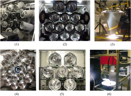
Light sources used in recent HFSS designs are most often xenon arc lamps (Bader, Haussener, and Lipiński 2015; Dai et al. 2019; Garrido et al. 2017; Gill et al. 2015; Janata 2002; Krueger, Davidson, and Lipiński 2011; Krueger, Lipiński, and Davidson 2013; Li et al. 2014; Li, Gonzalez-Aguilar, and Romero 2015; Li, Hu, and Lin 2022; Petrasch et al. 2007; Rowe et al. 2017; Sarwar et al. 2014; Wang et al. 2017; Wieghardt et al. 2016; Xiao et al. 2018), with several other designs using metal halide lamps (Codd et al. 2010; Dong et al. 2015; Dong et al. 2015; Ekman, Brooks, and Akbar Rhamdhani 2015; Lei et al. 2017; Roba and Siegel 2017), argon arc lamps (Hirsch et al. 2003; Melchior et al. 2008), and tungsten halogen lamps (Emery, Myers, and Rummel 1988). The vast majority concentrate the light with truncated ellipsoidal reflectors, though exceptions can be found using non-coaxial ellipsoid of revolution reflectors (Xiao et al. 2018), parabolic reflectors combined with a Fresnel lens (Wang et al. 2014; Wang et al. 2017; Zhu et al. 2020), or coupled and secondary parabolic mirrors (Varón et al. 2023). Multi-lamps simulators are also built with varying number of lamp modules (up to 149 Wieghardt et al. 2016) arranged in different orientations (hexagonal, circular, linear arrays (e.g. 3-4-3 pattern)), as well as surface quality and eccentricity of the reflector (Krueger, Davidson, and Lipiński 2011). Consequently, the peak flux values and flux profiles of the various HFSS designs vary according to design parameters. HFSSs with lamp modules arranged in different orientations are shown in Figure 1. Detailed surveys of existing HFSS designs can be found in Pottas et al. (2022), Gallo et al. (2017) and Liu et al. (2023).

Figure 1. HFSSs with different fonfigurations, (1) 12 lamp, 84 kWe xenon arc solar simulator at KTH, Sweden (Wang et al. 2017), (2) 12 lamp, 84 kWe xenon arc solar simulator at CAS, China (Dai et al. 2019), (3) 7 lamp, 10.5 kWe metal halide solar simulator at MIT (Codd et al. 2010), (4) 18 lamp, 45 kWe xenon arc solar simulator at ANU, Australia (Rowe et al. 2017), (5) 7 lamp, 42 kWe xenon arc solar simulator at IMDEA Energy Institute, Spain (Li, Gonzalez-Aguilar, and Romero 2015), (6) 75 kWe single argon arc solar simulator at ETH, Switzerland (Hirsch et al. 2003).

Before a HFSS is constructed, there is often a design procedure to select parameters like reflector geometry and number and position of modules. In many prior HFSS design studies, Monte Carlo Ray Tracing (MCRT) is used to simulate thermal radiation leaving the arc lamp, including the interaction with the reflector and ultimately its arrival at a target (Bader, Haussener, and Lipiński 2015; Ekman, Brooks, and Akbar Rhamdhani 2015; Gill et al. 2015; Jiang et al. 2020; Li et al. 2019; Li et al. 2020; Li, Gonzalez-Aguilar, and Romero 2015; Li, Hu, and Lin 2022; Milanese, Colangelo, and de Risi 2021; Petrasch et al. 2007; Varón et al. 2023; Wang et al. 2014; Zhu et al. 2020). Resulting radiative heat flux distributions are used to characterise the input that would be transferred to test article. After construction, the flux profile of a HFSS can be compared to simulations by experimental measurements using calibrated images of light reflected off a Lambertian target (Abuseada, Ophoff, and Ozalp 2019; Dai et al. 2019; Li et al. 2020; Li, Hu, and Lin 2022; Pottas et al. 2022; Sarwar et al. 2014; Varón et al. 2023) or with heat flux gage measurements at varying positions (Ekman, Brooks, and Akbar Rhamdhani 2015; Li, Hu, and Lin 2022; Zhu et al. 2020). Radiation transfer efficiency, the ratio between the power on a target and the source power is used to characterise the performance of the lamp-reflector array (Bader, Haussener, and Lipiński 2015; Ekman, Brooks, and Akbar Rhamdhani 2015; Jiang et al. 2020; Li et al. 2020; Petrasch et al. 2007; Sarwar et al. 2014; Zhu et al. 2020), though this value is difficult to compare across different studies because the calculation depends on the target selected, which can be planar (Ekman, Brooks, and Akbar Rhamdhani 2015; Jiang et al. 2020; Li et al. 2020; Li, Hu, and Lin 2022; Milanese, Colangelo, and de Risi 2021; Petrasch et al. 2007; Zhu et al. 2020) or hemispherical (Bader, Haussener, and Lipiński 2015; Li et al. 2019) of varying size, and the source power is sometimes defined as the electrical input (Ekman, Brooks, and Akbar Rhamdhani 2015; Li et al. 2020; Sarwar et al. 2014; Zhu et al. 2020) to the lamps (Ekman, Brooks, and Akbar Rhamdhani 2015; Li et al. 2020; Sarwar et al. 2014; Zhu et al. 2020) and sometimes as the radiation leaving the lamp arc (Bader, Haussener, and Lipiński 2015; Jiang et al. 2020). Typically, iterative MCRT simulations are performed with varied parameters. The goal is not usually to maximise transfer efficiency, but to provide sufficient target flux and acceptable transfer efficiency while considering constraints such as cost and hardware fabrication (Bader, Haussener, and Lipiński 2015; Jiang et al. 2020; Krueger, Lipiński, and Davidson 2013). Though many studies present the results of only a single lamp configuration (usually the as-built configuration) some investigation has been done into performance dependencies on varying design parameters, including number of lamps (Bader, Haussener, and Lipiński 2015), reflector eccentricity (Krueger, Davidson, and Lipiński 2011), lamp module position (Bader, Haussener, and Lipiński 2015), and focal length (Petrasch et al. 2007). Some authors provide flux distributions for individual lamps, allowing for a target flux distribution to be constructed from overlapping distributions from several lamps at various orientations to design the entire HFSS (Ekman, Brooks, and Akbar Rhamdhani 2015; Li et al. 2020; Li, Hu, and Lin 2022; Zhu et al. 2020). The effect of arc size (Li et al. 2020; Petrasch et al. 2007) and arc position in the reflector (Abuseada, Ophoff, and Ozalp 2019; Zhu et al. 2020) have also been investigated for their impact on the flux distribution. Investigations focusing on a single parameter variation are most common, but procedural methods to explore the impact of the flux distribution on multiple cross-interacting parameters of a HFSS would add great value to the design and optimisation process of HFSSs and enable highly flexible post-fabrication flux profile adjustment.

Although the HFSS design parameters mentioned above can be optimised to increase the transfer efficiency or peak flux of the simulator, they are generally designed to be unaltered once the simulator is built, with variability only though varying number of lamps operating or lamp power. The need for variability in flux profile from a single HFSS design is well noted in the literature.

Authors have discussed how research applications may require different flux orientations and concentrations for the following applications.

1. Testing of differently sized prototypes with variations in input power up to an order of magnitude, requiring varying focal plane spot sizes, currently achieved through defocusing and power adjustment which leads to low transfer efficiency and little control over uniformity (Liu et al. 2023)

2. Solar reactors for thermochemical processing designed with different absorber configurations and aperture orientations that rely on directionally diverse concentrated solar irradiation conditions (Li et al. 2019; Zhu et al. 2020)

3. Receiver material testing with a wide range of application temperatures (Li, Hu, and Lin 2022; Martínez-Manuel et al. 2018; Wang et al. 2017)

4. Linear flux to evaluate components of line-focusing technology like parabolic troughs (Li, Gonzalez-Aguilar, and Romero 2015).

A HFSS with flexibility to adjust the flux distribution on the focal plane will significantly widen the field of applications for a single device, and will be able to better mimic the distributions created by solar concentrating systems.

1.1. Development of HFSS with flux profile variability

Several research studies have investigated options for achieving variable flux profiles. With most HFSSs, the lamp power and number of lamps operating can be varied. The effect of lamp power has been quantified in several studies, finding that the magnitude of the entire flux distribution is scaled nearly linearly with lamp power for xenon arc lamps (Dai et al. 2019; Sarwar et al. 2014) and peak flux scales linearly with lamp power for argon arc lamps (Hirsch et al. 2003). Varying the number of lamps operating will change the peak flux and shape of the flux distribution (Bader, Haussener, and Lipiński 2015; Dai et al. 2019), though the shape effect is minor when all lamps share a common aimpoint at the target focal plane, as they do in most HFSSs. The flux distribution can also be varied by moving the target flux distribution plane or test article (Jiang et al. 2020; Wang et al. 2014). Jiang et al. (2020) found that the central irradiance diffused to the periphery and unevenness was reduced when the target was moved closer to the light source, with similar results shown by Wang et al. (Wang et al. 2014) when the target was moved away from the light source. While this can drastically alter the peak flux, average flux, and the shape of the distribution (Gallo et al. 2017), it affords no precise control – rather a set of flux distribution shapes to choose from at different target locations. Some analysis of HFSS flux distributions has led to rule-of-thumb guidelines, such as the determination by Petrasch et al. that the peak flux decays by a factor of 2 when the target object is moved every 50 mm of distance away from the target plane of a 10-lamp xenon arc HFSS with a focal length of 3 m (Petrasch et al. 2007).

Some systems, such as cavity receivers, may be primarily impacted by the total power on a specific aperture size, though variable flux profiles may help these systems avoid hot-spots or high thermal gradients. However, for other applications, especially those coupled to a specific real-world solar concentrator, it may be necessary to match or approximate a specific flux distribution with a HFSS, which can be achieved by adjusting lamp orientation and bulb position as well as lamp power and target location. Adjustment of the shape of the flux distribution through these parameters may open up new, more flexible experimental approaches from a single HFSS. Few studies have explored methods to systematically generate a desired flux profile in this way, though existing HFSSs have been built with hardware capability.

IMDEA Energy Institute in Spain built a HFSS consisting of seven-hexagonal xenon short arc lamps and attempted to achieve a variable flux distribution by adjusting the lamp orientation and conducted analysis on uniform line concentrated flux (Li, Gonzalez-Aguilar, and Romero 2015). A 70 kWe HFSS was built at the University of Chinese Academy of Sciences that can produce concentrated high flux, medium flux, and non-concentrated quasi-collimated light with adjustable power output. This variability in flux is achieved with the help of an optical integrator and a collimating lens (Jin, Hao, and Jin 2019). At the North China Electric Power University, China a flexible HFSS was built, for which the flux distribution in two-dimensional and three-dimensional space is achieved with the help of optical-fibre bundles, each placed at the focal point of an ellipsoidal reflector. The arrangement of the optical-fibre bundles can be varied based on the required output flux distribution (Song et al. 2019). A solar simulator designed at Harbin Institute of Technology, China considered replaceable Fresnel lenses as a means to modify the flux profile for various experiments (Jiang et al. 2020). A recent study by Pottas et al. showed that photogrammetry alignment of simulator modules can precisely allow for lamp module positions, though the simulator used requires manual adjustment (Pottas et al. 2022).

A HFSS was constructed at the Nanjing University of Aeronautics and Astronautics, in Nanjing, China, using 13 10-kWe xenon arc lamps with ellipsoidal reflectors (Zhu et al. 2020). Each lamp module was provided 3-axis adjustment to modify aim point and distance from the target. MCRT simulations were done to investigate the impact of arc position, showing that the flux distribution is highly sensitive to arc position relative to the reflector focal point. To improve uniformity, lamps were positioned so the arc was approximately 5 mm behind the focal point. Experimental investigations focused on further improving flux uniformity by adjusting lamp module aim points, module axial position, target position, and lamp power. Improvements were seen by adjusting aim points and lamp power or by moving the target forward of the target focal point. A HFSS built at the National University of Singapore included hardware adjustment of six degrees of freedom, including module position and aim direction, arc position, and reflector concentricity (Li et al. 2020). Adjustments were used to optimise transfer efficiency, but producing varied flux profiles, while noted, was outside the scope of the work. In many cases, HFSS designs even include at least 2-axis adjustment on the lamps (Dai et al. 2019; Milanese, Colangelo, and de Risi 2021), but the systems seem to be only used to bring all lamps to a common aim point. The largest HFSS in the world, SynLight at the German Aerospace Center, has 149 lamps, each with individual motion control in three degrees of freedom (Wieghardt et al. 2016), though, to date, no results of using this control for flux profile optimisation have been published.

1.2. Objectives of this work

Past studies have demonstrated both that there are potential applications of HFSSs with easily tunable flux profiles, and that the flux can be varied by changing geometric parameters of the lamp-reflector assembly (Dai et al. 2019; Milanese, Colangelo, and de Risi 2021). The majority of these studies focused on creating a uniform flux profile rather than producing disparate profiles, and generally investigated the effect, rather than the optimisation, of varying one or a limited set of parameters.

In the present work, we seek to develop a systematic method to produce arbitrary flux profiles by adjusting geometric and electrical parameters of lamp-reflector modules in multi-lamp HFSSs. While an example lamp and reflector are considered in our model demonstration, we present the full, generalised methodology with the modelling and parameterisation of the design so that the methodology is not specific to, or dependent on, any particular HFSS design. Future researchers can use the framework presented here to parameterise their own HSFF design and apply the presented optimisation method for producing target flux distributions.

It should be noted, that, although there will naturally be errors between the model optimised flux profile and the experimental flux profile, this work focuses on the procedure and capability of the parameterisation method and optimisation routine. Because levels of error and uncertainty are highly dependent on specific HFSS design choices, including lamp, reflector, and position control hardware, validation of flux profile prediction error is left for future work on specific HFSS designs.

2. Lamp module model development

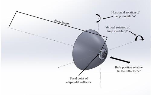
A lamp-reflector module is considered with the possibility of adjusting the flux profile through the following parameters, depicted in Figure 2:

1. Horizontal and vertical angle of the lamp modules with respect to a central axis of the simulator.

2. Motion of the bulb relative to the near focal point of the reflector

3. The radiative power emitted by the lamp arcs

Figure 2. Geometric parameters considered to analyse the variation in the flux profile are the rotation about horizontal and vertical axes defined from the focal point of the ellipsoidal reflector and the motion of the bulb along the focal axis away from the focal point.

The variation in the flux profile with respect to the parameters mentioned above is analysed using the MCRT technique. A variety of software have been used for MCRT analysis of HFSSs, including Opticad (Milanese, Colangelo, and de Risi 2021), FRED (Ekman, Brooks, and Akbar Rhamdhani 2015; Wang et al. 2017), Tonatiuh (Varón et al. 2023), Vegas (Li, Hu, and Lin 2022; Petrasch et al. 2007), TracePro (Li, Gonzalez-Aguilar, and Romero 2015; Roba and Siegel 2017; Xiao et al. 2018), and several others. In this work, TracePro, a non-sequential ray-tracing simulation software, is used for optical analysis of solid models. Rays, each associated with a specific radiative power and wavelength, are emitted from sources (the lamp arc in the current work) and propagated geometrically until intersection is found with an object. There, the ray can be subjected to absorption, reflection, refraction, diffraction, and scattering. Interactions are governed by random number generation, and many rays are necessary to converge to a physically accurate solution. To perform simulations, a solid model constituting of reflector, lamp bulb, and the target are created and properties of each are defined.

The reflector used in this work is an ellipsoid of revolution reflector with parameters shown in Table 1. The reflector material and spectral properties such as spectral reflectance, absorptance, and scattering behaviour are adopted from the one used by Roba et al. (Roba and Siegel 2017), to consider a reflector of the same material and manufacturer. A single, spectrum-weighted total reflectance is defined as a surface property to the reflector.

Table 1. Parameters of the ellipsoidal reflector modelled in MCRT simulations.

Ellipsoid of revolution reflector
Focal length	1585.21 mm
Eccentricity	0.92
Rear hole diameter	140 mm
Rim angle	39.91 degrees
Reflectance	0.896
Absorptance	0.004
BRDF (A, B, g)	(0.00129, 0.015, 0)
Model and manufacturer	Optiforms E1585

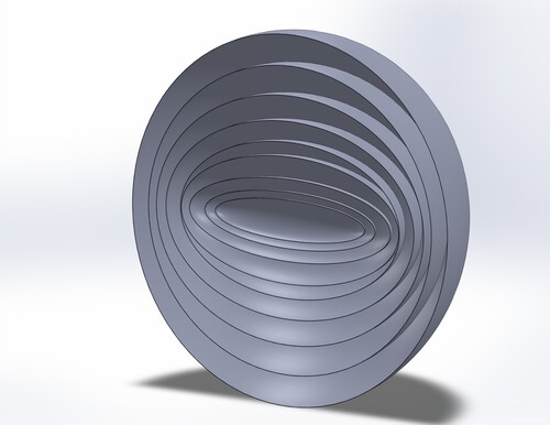
The bulb considered in this project is a Philips MSR Gold 2500 W metal halide lamp. The optical model of the arc source is one of the most important factors in accurately representing the actual solar simulator. Past studies have used a variety of approximations to account for the spatial variation of light emitted from a HID lamp arc, including a uniform cylinder (Bader, Haussener, and Lipiński 2015; Ekman, Brooks, and Akbar Rhamdhani 2015; Gill et al. 2015; Jiang et al. 2020; Li et al. 2020; Li, Hu, and Lin 2022; Zhu et al. 2020), a series of point sources (Milanese, Colangelo, and de Risi 2021), or a detailed 3-dimensional model generated through arc imaging (Wang et al. 2014). The smaller arc of xenon arc lamps leads to relatively minor errors from a highly simplified arc model. However, care must be taken for the arc model of metal halide lamps, which have larger arcs. Roba et al.’s approach is adopted, where the arc source is modelled as several nested surface sources with varying power and intensity (Roba and Siegel 2017). The present arc source model consists of nine coaxial ellipses, and can be seen in Figure 3. The major and minor diameter and power assigned to each shell are defined in (Roba and Siegel 2017).

Figure 3. Sectional view of the nested ellipsoid source model accounting for the spatial variation of radiation emission intensity.

In order to capture the flux profile obtained at the far focal point of the ellipsoidal reflector, the target is defined as a square plane, and the side of the target facing the lamp module is modelled as a perfect absorber.

A single lamp module normal to the target is modelled as shown in Figure 4. The bulb encasing the arc source is modelled as quartz. A convergence study is performed to understand the error in the flux profile obtained on the target surface due to number of rays. The peak flux is measured with increasing number of rays, and is found to converge at 300 million rays, where the number of rays emitted from each shell is 33.3 million. An increase in ray count from 200 million to 300 million results in a 0.6% change in peak flux, while increasing further to 400 million results in 0.02% change in peak flux. The number of rays per MCRT simulation is maintained throughout this study at 300 million.

Figure 4. Lamp module normal to the target, defined in TracePro.

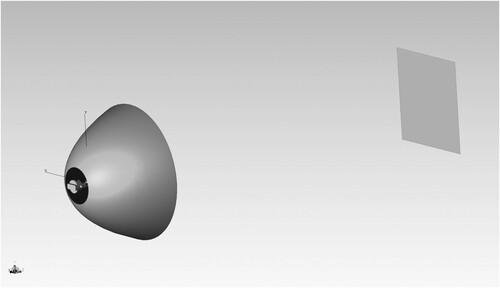
After defining the solid models and their respective properties, the MCRT simulation is performed with 300 million rays with the lamp module normal to the target. The flux profile obtained is shown in Figure 5(a).

Figure 5. Radiative heat flux profile at the target plane when lamp module is normal to the target: (a) two-dimensional, (b) one-dimensional centre cross-section.

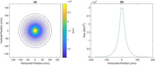
The one-dimensional flux profile, shown in Figure 5(b) is the sectional view of the flux profile at the centre of the target (flux intensities over the horizontal range of pixels at the vertical mid-point of the target).

The flux distribution on the target is axisymmetric and the flux profile is similar to a gaussian distribution, reaching a peak flux of 299 $\mathrm{kW}/{\mathrm{m}}^2$, and a total power of 1115.7 W on a 350×350 mm target achieving a transfer efficiency of 55.78% and accounting for the lamp efficiency of 80% (2000 W radiative power). Experimental validation of flux profiles generated from TracePro MCRT using an identical lamp and similar reflector is provided in the past work by Roba et al. (Roba and Siegel 2017), from which we have matched material properties and the lamp model.

3. Parameterising the flux profile

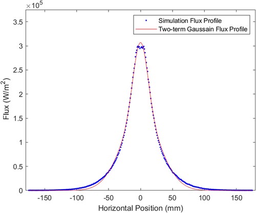
Automated optimisation of the HFSS flux profile requires the ability to generate flux profiles of individual lamps with varying parameters in far less time than would be required to complete ray tracing simulations for each case. Therefore, a parametric flux profile model is generated, which can quickly return an approximate flux profile for any set of lamp parameters within a specified range. Initially, a one-dimensional cross section of the flux profile is parameterised by fitting a two-term gaussian equation, (1) $I=a_1\ast \left(e^{-{\left({\displaystyle \frac{x}{c_1}}\right)}^2}+e^{-{\left({\displaystyle \frac{x}{c_2}}\right)}^2}\right)$(1) where a₁ is half of the peak flux value, in $\mathrm{W}/{\mathrm{m}}^2$. Eq. (1) consists of the sum of two-gaussian equations, and the parameters c₁ and c₂, in mm, are used to define the kurtosis of the flux profile. The comparison between the two-gaussian equation fit and the simulated flux profile is shown in Figure 6. The area under the one-dimensional flux profile provides the power delivered on the target at an area of 1×350 mm. The simulated flux-profile delivers a power of 16.18 W and the power delivered by the two-term gaussian equation is 15.75 W. The R-squared value of the fit is 0.998, proving good agreement between the simulated flux profile and the two-term gaussian equation.

Figure 6. One-dimensional curve fit of the radiative flux profile, showing that the two-term gaussian equation (solid) provides a close approximation to the simulated one-dimensional flux profile (dotted).

The two-dimensional flux profile is parameterised by fitting the same two-term gaussian equation to the horizontal cross-sections at each vertical position on the target. Thus, Eq. (1) is fit to a series of one-dimensional flux profiles, and the variation in parameters a₁, c₁, and c₂ with respect to vertical distance from target centre (vertical position) can be examined. The variation in these parameters at vertical distances from −175 mm to 175 mm when the lamp module is normal to the target is shown in Figure 7.

Figure 7. Parameter a₁, c₁, and c₂ with respect to vertical position on the target, a₁ represents the peak intensity c₁ and c₂ are used to define the kurtosis of the flux profile. Blue dots indicate a₁, c₁, and c₂ generated through curve fitting of individual horizontal slices of the flux profile and the red lines indicate the curve fits to these parameters using the two-term gaussian equation.

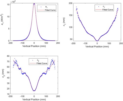
The variation in parameters a₁, c₁, and c₂ are now further parameterised by fitting the relationships. Parameter a₁ is fit with same two-term gaussian equation shown in Eq. (1). The coefficients resulting from this fit are a₁₁, c₁₁ and c₂₁, as shown in Eq. (2). Parameters c₁ and c₂ are fit with the equations Eq. (3) and Eq. (4). The results of these fits can be seen in Figure 7. These equations provide the variation in the curve fit parameters as position of the one-dimensional flux profile is changed in the vertical direction, (2) $a_1=a_{11}\ast \left(e^{-{\left({\displaystyle \frac{y}{c_{11}}}\right)}^2}+e^{-{\left({\displaystyle \frac{y}{c_{21}}}\right)}^2}\right)$(2) (3) $c_1=a{c}_1\ast \left(e^{b{c}_1\ast y}+e^{-b{c}_1\ast y}\right)+c{c}_1\ast e^{-{\left({\displaystyle \frac{y}{d{c}_1}}\right)}^2}$(3) (4) $c_2=a{c}_2\ast \left(e^{b{c}_2\ast y}+e^{-b{c}_2\ast y}\right)+c{c}_2\ast e^{-{\left({\displaystyle \frac{y}{d{c}_2}}\right)}^2}$(4)

Thus, the entire two-dimensional flux profile for a single lamp orientation can be approximately recreated by finding best fit values of the 11 parameters a₁₁, c₁₁, c₂₁, ac₁, bc₁, cc₁, dc₁, ac₂, bc₂, cc₂, dc₂.

4. HFSS surrogate model development

The set of parameters discussed above serves as the information necessary to recreate a flux profile for a single lamp and bulb orientation. However, a full model for the HFSS requires the values of the 11 parameters at a variety of orientations. The complete HFSS surrogate model is developed by analysing the variations in the parameters mentioned in the previous section in response to changes in the geometric parameters of the HFSS mentioned in section 1.1.

4.1. Rotation of lamp modules about horizontal and vertical axes

In a multi-lamp HFSSs, each lamp in the array is positioned with a given angle between the reflector axis and the central axis of the HFSS. If the target is fixed normal to the entire HFSS axis, the value of this angle will change the flux profile from an individual lamp, and how the flux profile responds to rotation of the lamp module. Therefore, to develop a complete model of a specific solar simulator, simulations would be performed for each unique angle at which lamps are located. This can be very time consuming, so to demonstrate the process, it is assumed that the modelled HFSS is composed of ten lamps all located at the centre of the array and nominally normal to the target. Essentially all ten lamps are assumed to be in the same location. This is rather an impractical case but will help in assessing the possibility of the optimisation of the HFSS flux distribution.

The range selected for lamp rotation is 10 degrees about either the horizontal or vertical axes. This range allows target focal points to fall in a 300 mm by 300 mm target space. This experimental area is typical of most high temperature thermal and thermochemical research applications for a 25 kWe HFSS. Though a wider target space could be modelled with greater rotation, more simulations are necessary for equal accuracy, and distributions on a larger area are rarely needed. The lamp module is rotated with respect to axes through the arc-source focal point, and a relationship is determined between the 11 parameters and the rotation angle about horizontal and vertical by performing polynomial least-squares regression analysis. The property of symmetry is applied where the lamp module is swiveled only in the positive angle quadrant and the obtained variation in flux profile is mirrored to the rest of the quadrants.

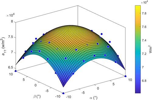
Example variation in two parameters, a₁₁ and c₁₁, with rotation about the vertical axis is given in Figure 8. The variation of constant a₁₁ with respect to both horizontal and vertical swivel angle can be a seen in Figure 9. The rest of the 10 parameters are analysed using the same 5-degree polynomial equation and their respective coefficients are used to define the HFSS model. The entire flux profile for a single lamp at any aim point on the target can now be obtained using constants. Extensive results from curve fitting of all parameters can be found in (Hossein 2019) and online access to the raw data is located at 10.5281/zenodo.11372420.

Figure 8. Regression analysis between the constant a₁₁ & c₁₁ and the lamp module rotation angle about the vertical axis, blue dots indicate simulated values.

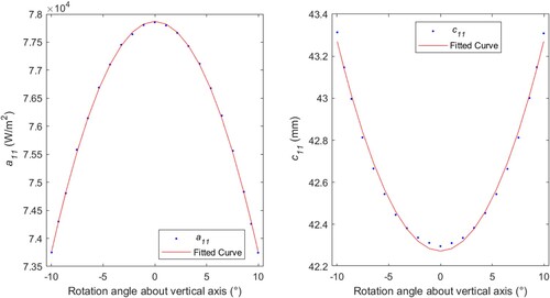
Figure 9. Parameter a₁₁ with respect to rotation angles α and β. Blue dots indicate simulated values, and the surface is a polynomial curve fit of degree 5.

4.2. Motion of the bulb with respect to the near focal point of the reflector

In this section, the metal halide bulb is simulated at positions near the focal point along the focal axis of the reflector, with position indicated by parameter δ. Positive δ indicates the bulb is moved towards the target focus. The variation in the flux profile is analysed. One observation made is that when the lamp module is moved more than ± 6.5 mm away from the focal point of the ellipsoidal reflector, the flux profile no longer follows a gaussian distribution and is difficult to parameterise using the equations provided in Section 3. Hence, the position of the bulb is limited to ± 6.5 mm from the focal point of the reflector. The variations of all fit parameters are captured. The variation in constant a₁₁ can be seen in Figure 10 as an example, with other fits presented in (Hossein 2019). The peak flux is slightly lower when the lamp module is moved in the negative direction than when it is moved in the positive direction from the focal point, due to higher radiation energy loss to the rear aperture of the ellipsoidal reflector.

Figure 10. Variation in parameter a₁₁ with respect to bulb position.

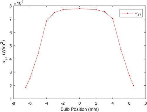
The level of decrease in flux at the target with the motion of the bulb is similar at all angles of the lamp module. Hence, the variation in the 11 parameters with respect to the motion of the bulb are normalised with respect to when the bulb is at the focal point of the reflector (δ = 0 mm) and are added as a scaling coefficient to the previously obtained variation in the parameters, mentioned in section 4.1.

4.3. Varying the power of the lamp module

The selected metal halide lamps of the HFSS can either be switched off or can be operated from 50–100% of their rated power. The flux profile is expected to vary linearly with respect to the power supplied to each lamp module (Sarwar et al. 2014).

The variation in the flux profile with respect to variation in the power to the lamp module is defined as a single parameter, $P_i$, where i is the lamp module number, and $P_i$ can either be 0 or can be any value between 0.5-1.0.

4.4. Flux profile of the solar simulator

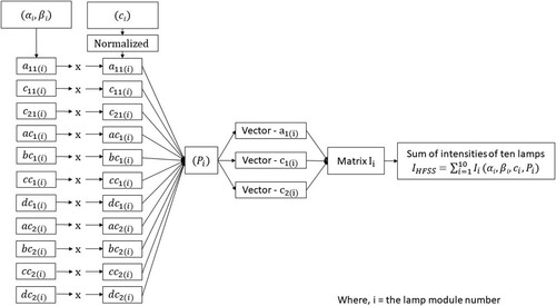
The flux intensity profile of the solar simulator is found for a given set of the parameters α_i, β_i, δ_i, and P_i for each of the i lamp modules in the array. First, the curve fits developed above are applied to identify the 11 fit parameters for the input α and β values. The fit parameters are scaled according to the relationship with δ. The 11 fit parameters then determine vectors of one-dimensional fit parameters a₁, c₁, and c₂, which are scaled by the lamp power P_i. These parameters then determine a matrix of intensities for each lamp, which are summed to determine the flux intensity profile of the HFSS. A flow-chart of the process is shown in Figure 11.

Figure 11. Flux profile surrogate model structure for the 10 lamp HFSS.

5. Optimisation of HFSS

In this section, a method is discussed to determine parameters of the lamp modules which will achieve a desired flux profile. A trust-region reflective algorithm (Conn, Gould, and Toint 2000) is applied to the developed HFSS model with the goal of minimising the linear difference between a user defined flux profile and the flux profile generated by the HFSS. The optimisation algorithm receives an input of a user-defined, or target, flux profile and the initial parameter set of the HFSS. The output of the algorithm is as set of angles about the vertical α and horizontal β axes, bulb position δ, and the power P to each lamp module required to achieve a HFSS flux profile which closely approximates the user-defined flux-profile.

5.1. Implementation of trust-region reflective algorithm to the HFSS model

The constraints applied to the optimisation algorithm are as follows:

1. Each lamp module is allowed to rotate only from −10 degrees to 10 degrees,

2. The arc of the bulb is allowed to move from −6.5 mm to 6.5 mm and

3. The power factor of each lamp module can either be zero or can be anywhere within [0.5-1.0].

The side constraint for the power to each lamp module is a step-function in nature. Due to this nature, the output of the optimisation becomes very much dependent on the initial power levels defined as the input to the optimisation algorithm. For example, if the initial point is defined in such a way that the power to the lamp #1 is zero and the rest of the lamp modules are given the initial operating power of 100%, the optimisation method converges with lamp #1 power being zero and with varying operating power levels to the rest of the lamp modules, without considering switching off other lamp modules.

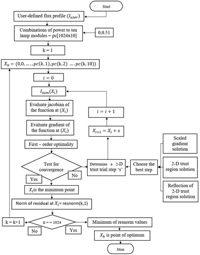
Due to this condition, the optimisation algorithm is run for every combination of lamps switched on (at P_i= 0.5) or off. Hence there are $2^{10}$ = 1024 possibilities of state combinations of the lamp modules. The optimisation model is run 1024 times, and in each iteration a different combination of on/off states for the ten lamp modules is given as an initial point for the trust region reflective algorithm. The lowest residual norm value obtained is considered as the optimum configuration. Residual norms for each lamp switching combination are computed by running the trust-region reflective algorithm to convergence and recording the HFSS state and residual norm value. The working of the optimisation technique is visualised in the flow chart shown in Figure 12.

Figure 12. Flow chart of trust-region reflective optimisation algorithm.

5.2. Testing the optimisation of HFSS to achieve a uniform user-defined flux profile

Many HFSS studies discuss the benefits of a flux profile that is relatively uniform over a specific area, and attempts have been made to improve uniformity, both in the design stage by increasing the number of lamps (Bader, Haussener, and Lipiński 2015), and in the operational stage by moving the bulb or target (Li et al. 2020; Zhu et al. 2020), or by adding additional devices like homogenisers (Li, Hu, and Lin 2022) or non-imaging secondary concentrators (Li et al. 2019). To test the ability of the optimisation algorithm to create such a profile by varying lamp aim point, bulb position, and lamp power, a uniform flux profile is defined as an input to the algorithm that has an intensity of 0.5 ($\mathrm{MW}/{\mathrm{m}}^2$) covering an area of 130 mm x 130 mm at the centre of the experimental area. The optimisation algorithm converges with the configuration where all the lamps are powered on (1024th power combination) and takes 146 iterations in that particular power combination, with a resultant normal value 6.64E+14. The results can be seen in Table 2. The comparison between the flux profile of the solar simulator and the user-defined flux profile is shown in Figure 13.

Figure 13. Uniform user-defined flux profile and the flux profile output of the optimisation algorithm.

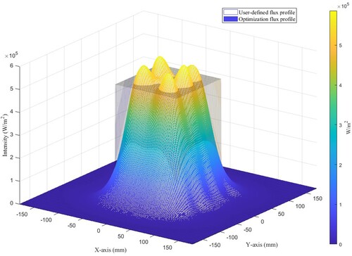
Table 2. Optimisation algorithm output configuration – uniform flux profile.

Lamp module	Rotation about vertical axis (°)	Rotation about horizontal axis (°)	Bulb position (mm)	Power (%)
1	0.43	1.40	−0.61	0.94
2	−0.49	−1.41	−0.65	0.93
3	1.24	−0.96	−0.82	0.94
4	−1.34	1.57	−0.80	0.99
5	−1.25	−0.26	−0.87	0.99
6	−1.50	−1.51	−0.88	1.00
7	1.49	1.50	0.78	1.00
8	−1.26	0.98	−0.83	0.90
9	1.32	−1.58	−0.80	1.00
10	1.26	0.30	−0.85	0.96

The algorithm does not force a match to peak or average flux between the defined and achieved flux profiles, but minimises the area integrated residual. As expected, if attempting to produce a uniform flux profile using Gaussian-type profiles, areas near the centre have higher flux than desired, while the edge of the distribution has lower flux than desired. However, in comparison to the flux profile of a 10-lamp HFSS with a common aim point, even with defocusing, the optimised distribution shown is far closer to the target distribution. The optimised result includes a moderate de-focusing of all lamps, while power for all lamps is above 90% of maximum power. The peak flux obtained by the optimisation output is 0.66 ($\mathrm{MW}/{\mathrm{m}}^2$), which is 0.16 ($\mathrm{MW}/{\mathrm{m}}^2$) higher than the user defined peak flux, which would result in hot spots on the target surface along with a maximum flux outside of the defined high-flux area of 0.283 ($\mathrm{MW}/{\mathrm{m}}^2$). The aimpoints of the lamp modules essentially form a rectangle, with four lamps at full power aiming at the corners and the other six lamps aiming at points along the lines connecting the corners. No lamps are aimed at the centre of the profile. However, this may not be the case if the number of lamps were greater. More lamps are also likely to lead to a better overall fit as well. Compared to methods that only attempt to optimise peak flux or power on an area, this method also factors in flux outside of defined high-flux area, and seeks to minimise this spillage radiation, improving transfer efficiency and energy consumption for a given experiment. Total power is not forced to match with this algorithm. The power defined by the user-defined uniform flux profile is 10510 W and the power output of the optimisation algorithm is 9152.5 W, showing a difference of 1357.5 W, a difference of 13%.

5.3. Testing the optimisation of HFSS to achieve an ellipsoidal user-defined flux profile

For device experimentation meant to mimic flux conditions from real-world concentrators, non-uniform flux distributions are likely more realistic. The optimisation algorithm is capable of optimising the flux profile to match any user defined flux profile shape. To demonstrate, an ellipsoidal user-defined flux profile is defined as an input. It has a peak intensity of 0.42 $\mathrm{MW}/{\mathrm{m}}^2$ with a major axis of 280 mm (−140 mm to 140 mm) and minor axis of 160 mm (−80 mm to 80 mm) at the centre of the experimental area. The optimisation algorithm converges with the configuration where all the lamps are powered on as shown in the Table 3. The comparison between the flux profile of the solar simulator and the user-defined flux profile is shown in in Figure 14. Six lamps are operated with relatively high power and some de-focusing at approximately 80% of maximum power, while two lamps are located at the tail ends of the ellipse with approximately 70% power. The final two lamps are highly defocused and aimed near the centre of the distribution at approximately 50% power to help smooth the overall distribution.

Figure 14. Ellipsoidal user-defined flux profile and the flux profile output of the optimisation algorithm.

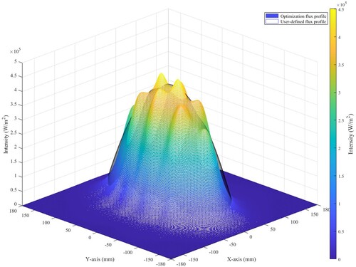
Table 3. Optimisation algorithm output configuration – ellipsoidal flux profile.

Lamp module	Rotation about vertical axis (°)	Rotation about horizontal axis (°)	Bulb position (mm)	Power (%)
1	−0.95	1.83	−0.82	0.79
2	0.99	1.83	−0.82	0.79
3	0.01	0.79	−2.76	0.51
4	0.02	3.27	0.64	0.67
5	1.14	0.02	0.78	0.83
6	0.01	−3.22	0.67	0.68
7	0.00	−0.75	−2.75	0.51
8	0.99	−1.79	−0.84	0.79
9	−0.96	−1.79	−0.85	0.78
10	−1.12	0.02	0.78	0.83

The peak flux obtained by the optimisation output is 0.451 ($\mathrm{MW}/{\mathrm{m}}^2$), which is 0.031 ($\mathrm{MW}/{\mathrm{m}}^2$) higher than the user defined peak flux. The peak flux outside the desired flux area is 0.052 ($\mathrm{MW}/{\mathrm{m}}^2$). The power defined by the user-defined ellipsoidal flux profile is 7389 W and the power output of the optimisation algorithm is 7741.2 W, showing a difference of 352.2 W or 4.5%.

6. Discussion

The results of the example profile optimisations, in Figures 13 and 14 show that the ellipsoidal flux profile is fit much better than the uniform distribution. The avoidance of step changes in the flux profile makes it much easier for the optimisation algorithm to match the flux near the edges of the non-zero portion of the distribution. Even for a fully focused lamp, there exists a maximum flux gradient. Target gradients which exceed this gradient will be challenging for a simulator to recreate, whether optimised or not. However, the demonstrated algorithm can find parameter sets which achieve close approximations to a wide variety of flux distributions. With a larger number of lamps, both edge gradients and overall fit will be improved. Due to the increase in fit quality and additional challenge of manual adjustment, the current method is more valuable for larger numbers of lamps in the array. For the two test cases, the optimisation routine did not appear to have a significant bias towards any of the variable parameters. Individual lamp power, bulb position with respect to the focal position, and rotation about both axes all proved to be parameters tuned by the optimisation algorithm in order to best match the target flux profile, indicating that it is unlikely that a manual trial-and-error approach would yield results with as strong fits.

The methodology presented here can be applied to any multi-lamp HFSS with the goal of matching a two-dimensional flux profile at a specific plane. Researchers must be able to effectively generate flux distributions of individual lamp reflector combinations at a wide variety of adjusted positions using MCRT or by experimental measurements. In this work, an example lamp arc model and reflector properties were used for demonstration, but, for HFSSs with different hardware, new flux profiles must be generated for input to the parameterisation. While only a single lamp is considered here, past studies have shown that flux distributions of several types of individual HFSS lamps generally are fit well with Gaussian distributions (Dai et al. 2019; Sarwar et al. 2014), so we expect that the method and equations for parameterisation can be repeated with similar fit for other HID lamp and elliptical reflector combinations. It is possible that alternative fit equations may produce better quality parameterisation if vastly different lamps or reflectors are used. The parameterisation method inherently introduces a level of error to the resulting optimised flux profile prediction. Future work will evaluate the production of flux distributions experimentally, although these evaluations are highly hardware dependent, with significant differences expected based on the lamp, reflector, and adjustment methods.

Once the flux profiles are parameterised, researchers can follow the presented methodology for trust-region reflective optimisation against a target flux profile of any shape, which can be defined by a mathematical equation or a numerical discretisation. The selected optimisation method is stable and is applicable to varying number of input parameters (i.e. varying number of lamps or adjustment constraints). The primary limitation is the inability to inherently handle the lamp on/off condition, though our method includes considering this fully by optimising at each combination of lamp on/off state and selecting the most optimised result. Even with this process, the optimisation method, implemented in the Matlab environment, requires only minutes to run. Generating the flux profiles with MCRT is the most time-intensive portion of the complete process.

7. Conclusion

Multi-lamp HFSSs can produce variable flux profiles through a variety of adjustments. The results in this work show how varying multiple parameters in conjunction can allow for close matches to a wide range of flux profiles, enabling expanded utility from a single HFSS. While many HFSSs are now being built with the ability to adjust many geometric parameters, some even with motorised adjustment, procedural optimisation of parameters to produce specific flux profiles has not been demonstrated. In this work, it was found that, given a complete set of single-lamp flux profiles, two-term Gaussian functions fit well to parameterise the flux distributions so a multi-lamp flux distribution can be generated parametrically. Then a trust-region reflective optimisation algorithm can be used to match this resulting profile to an objective profile. Doing so may automate the process of tailoring the adjustment of a HFSS for various experiments. Especially in a high-use facility with disparate experimental flux conditions, this could improve the throughput of the facility, improve flux conditions at device apertures to avoid hotspots and gradients, provide better tailored flux input and allow for irradiation more representative of concentrated sunlight. Future work should include applying the parameterisation and optimisation methods to experimental hardware and a wide variety of HFSS designs.

Acknowledgements

The authors would like to thank Nathan Siegel of Bucknell University for assistance in developing the ray-tracing model and providing input on the design of a metal–halide solar simulator.

Disclosure statement

No potential conflict of interest was reported by the author(s).

Data availability statement

All data from this work is available upon request to the corresponding author. Matlab codes and a full set of curve fits used for surrogate model development are hosted at: [To be archived upon article acceptance].

Additional information

Funding

This research did not receive any specific grant from funding agencies in the public, commercial, or not-for-profit sectors.

References

- Abuseada, M., C. Ophoff, and N. Ozalp. 2019. “Characterization of a New 10 kWe High Flux Solar Simulator Via Indirect Radiation Mapping Technique.” Journal of Solar Energy Engineering 141 (2): 021005. https://doi.org/10.1115/1.4042246.
- Ahmad, S. Q. S., R. J. Hand, and C. Wieckert. 2014. “Use of Concentrated Radiation for Solar Powered Glass Melting Experiments.” Solar Energy 109: 174–182. https://doi.org/10.1016/j.solener.2014.08.007.
- Bader, R., S. Haussener, and W. Lipiński. 2015. “Optical Design of Multisource High-Flux Solar Simulators.” Journal of Solar Energy Engineering 137 (2): 021012. https://doi.org/10.1115/1.4028702.
- Biswas, D., T. Cox, and J. L. Lapp. 2022. “Sintering Behavior of Lunar Soil Heated by Indirect and Direct Concentrated Sunlight” In ASME 2022 16th International Conference on Energy Sustainability, American Society of Mechanical Engineers. https://doi.org/10.1115/ES2022-81630.
- Codd, D. S., A. Carlson, J. Rees, and A. H. Slocum. 2010. “A low Cost High Flux Solar Simulator.” Solar Energy 84 (12): 2202–2212. https://doi.org/10.1016/j.solener.2010.08.007.
- Conn, A. R., N. I. M. Gould, and P. L. Toint. 2000. Trust Region Methods. Society for Industrial and Applied Mathematics.
- Dai, S., Z. Chang, T. Ma, L. Wang, and X. Li. 2019. “Experimental Study on Flux Mapping for a Novel 84 kWe High Flux Solar Simulator.” Applied Thermal Engineering 162: 114319. https://doi.org/10.1016/j.applthermaleng.2019.114319.
- Dong, X., G. J. Nathan, Z. Sun, D. Gu, and P. J. Ashman. 2015a. “Concentric Multilayer Model of the arc in High Intensity Discharge Lamps for Solar Simulators with Experimental Validation.” Solar Energy 122: 293–306. https://doi.org/10.1016/j.solener.2015.09.004.
- Dong, X., Z. Sun, G. J. Nathan, P. J. Ashman, and D. Gu. 2015b. “Time-resolved Spectra of Solar Simulators Employing Metal Halide and Xenon arc Lamps.” Solar Energy 115: 613–620. https://doi.org/10.1016/j.solener.2015.03.017.
- Ekman, B. M., G. Brooks, and M. Akbar Rhamdhani. 2015. “Development of High Flux Solar Simulators for Solar Thermal Research.” Solar Energy Materials and Solar Cells 141: 436–446. https://doi.org/10.1016/j.solmat.2015.06.016.
- Emery, K., D. Myers, and S. Rummel. 1988. “Solar simulation-problems and solutions,” in Conference Record of the Twentieth IEEE Photovoltaic Specialists Conference, IEEE, pp. 1087–1091. https://doi.org/10.1109/PVSC.1988.105873.
- Gallo, A., A. Marzo, E. Fuentealba, and E. Alonso. 2017. “High Flux Solar Simulators for Concentrated Solar Thermal Research: A Review.” Renewable and Sustainable Energy Reviews 77: 1385–1402. https://doi.org/10.1016/j.rser.2017.01.056.
- Garrido, J., L. Aichmayer, W. Wang, and B. Laumert. 2017. “Characterization of the KTH High-Flux Solar Simulator Combining Three Measurement Methods.” Energy 141: 2091–2099. https://doi.org/10.1016/j.energy.2017.11.067.
- Gill, R., E. Bush, P. Haueter, and P. Loutzenhiser. 2015. “Characterization of a 6 kW High-Flux Solar Simulator with an Array of Xenon arc Lamps Capable of Concentrations of Nearly 5000 Suns.” Review of Scientific Instruments 86 (12): 125107. https://doi.org/10.1063/1.4936976.
- Hathaway, B. J., and J. H. Davidson. 2017. “Demonstration of a Prototype Molten Salt Solar Gasification Reactor.” Solar Energy 142: 224–230. https://doi.org/10.1016/j.solener.2016.12.032.
- Hirsch, D., P. v. Zedtwitz, T. Osinga, J. Kinamore, and A. Steinfeld. 2003. “A New 75 kW High-Flux Solar Simulator for High-Temperature Thermal and Thermochemical Research.” Journal of Solar Energy Engineering 125 (1): 117–120. https://doi.org/10.1115/1.1528922.
- Hossein, M. H. 2019. “Variable Flux Profile Optimization of a High Flux Solar Simulator,” M.S., University of Maine, Orono. Accessed August 21, 2023. https://digitalcommons.library.umaine.edu/etd/3807.
- Janata, E. 2002. “A Pulse Generator for Xenon Lamps.” Radiation Physics and Chemistry 65 (3): 255–258. https://doi.org/10.1016/S0969-806X(02)00261-X.
- Jiang, B., B. Guene Lougou, H. Zhang, W. Wang, D. Han, and Y. Shuai. 2020. “Analysis of High-Flux Solar Irradiation Distribution Characteristic for Solar Thermochemical Energy Storage Application.” Applied Thermal Engineering 181: 115900. https://doi.org/10.1016/j.applthermaleng.2020.115900.
- Jin, J., Y. Hao, and H. Jin. 2019. “A Universal Solar Simulator for Focused and Quasi-Collimated Beams.” Applied Energy 235: 1266–1276. https://doi.org/10.1016/j.apenergy.2018.09.223.
- Krueger, K. R., J. H. Davidson, and W. Lipiński. 2011. “Design of a New 45 kWe High-Flux Solar Simulator for High-Temperature Solar Thermal and Thermochemical Research.” Journal of Solar Energy Engineering 133 (1): 011013. https://doi.org/10.1115/1.4003298.
- Krueger, K. R., W. Lipiński, and J. H. Davidson. 2013. “Operational Performance of the University of Minnesota 45 kWe High-Flux Solar Simulator.” Journal of Solar Energy Engineering 135 (4): 044501. https://doi.org/10.1115/1.4023595.
- Lapp, J. L., M. Lange, R. Rieping, L. de Oliveira, M. Roeb, and C. Sattler. 2017. “Fabrication and Testing of CONTISOL: A new Receiver-Reactor for day and Night Solar Thermochemistry.” Applied Thermal Engineering 127: 46–57. https://doi.org/10.1016/j.applthermaleng.2017.08.001.
- Lei, F., P. Dupuis, O. Durrieu, G. Zissis, and P. Maussion. 2017. “Acoustic Resonance Detection Using Statistical Methods of Voltage Envelope Characterization in Metal Halide Lamps.” IEEE Transactions on Industry Applications 53 (6): 5988–5996. https://doi.org/10.1109/TIA.2017.2742978.
- Li, X., J. Chen, W. Lipiński, Y. Dai, and C.-H. Wang. 2020. “A 28 kWe Multi-Source High-Flux Solar Simulator: Design, Characterization, and Modeling.” Solar Energy 211: 569–583. https://doi.org/10.1016/j.solener.2020.09.089.
- Li, J., J. Gonzalez-Aguilar, C. Pérez-Rábago, H. Zeaiter, and M. Romero. 2014. “Optical Analysis of a Hexagonal 42kWe High-Flux Solar Simulator.” Energy Procedia 57: 590–596. https://doi.org/10.1016/j.egypro.2014.10.213.
- Li, J., J. Gonzalez-Aguilar, and M. Romero. 2015. “Line-concentrating Flux Analysis of 42kWe High-Flux Solar Simulator.” Energy Procedia 69: 132–137. https://doi.org/10.1016/j.egypro.2015.03.016.
- Li, J., J. Hu, and M. Lin. 2022. “A Flexibly Controllable High-Flux Solar Simulator for Concentrated Solar Energy Research from Extreme Magnitudes to Uniform Distributions.” Renewable and Sustainable Energy Reviews 157: 112084. https://doi.org/10.1016/j.rser.2022.112084.
- Li, L., B. Wang, R. Bader, J. Zapata, and W. Lipiński. 2019a. “Reflective Optics for Redirecting Convergent Radiative Beams in Concentrating Solar Applications.” Solar Energy 191: 707–718. https://doi.org/10.1016/j.solener.2019.08.077.
- Li, L., B. Wang, J. Pottas, and W. Lipiński. 2019b. “Design of a Compound Parabolic Concentrator for a Multi-Source High-Flux Solar Simulator.” Solar Energy 183: 805–811. https://doi.org/10.1016/j.solener.2019.03.017.
- Liu, L., G. Sun, G. Zhang, S. Liu, and J. Zhang. 2023. “Research Progress in High-Flux Solar Simulators.” Applied Thermal Engineering 224: 120107. https://doi.org/10.1016/j.applthermaleng.2023.120107.
- Manzoor, M. T., L. Peinturier, and M. Tetreault-Friend. 2023. “Concrete Based Molten Salt Storage Tanks.” J Energy Storage 57: 106151. https://doi.org/10.1016/j.est.2022.106151.
- Martínez-Manuel, L., et al. 2018. “A 17.5 KWel High Flux Solar Simulator with Controllable Flux-Spot Capabilities: Design and Validation Study.” Solar Energy 170: 807–819. https://doi.org/10.1016/j.solener.2018.05.088.
- Melchior, T., C. Perkins, A. W. Weimer, and A. Steinfeld. 2008. “A Cavity-Receiver Containing a Tubular Absorber for High-Temperature Thermochemical Processing Using Concentrated Solar Energy.” International Journal of Thermal Sciences 47 (11): 1496–1503. https://doi.org/10.1016/j.ijthermalsci.2007.12.003.
- Milanese, M., G. Colangelo, and A. de Risi. 2021. “Development of a High-Flux Solar Simulator for Experimental Testing of High-Temperature Applications.” Energies 14 (11): 3124. https://doi.org/10.3390/en14113124.
- Petrasch, J., et al. 2007. “A Novel 50 kW 11,000 Suns High-Flux Solar Simulator Based on an Array of Xenon Arc Lamps.” Journal of Solar Energy Engineering 129 (4): 405–411. https://doi.org/10.1115/1.2769701.
- Pottas, J., L. Li, M. Habib, C.-H. Wang, J. Coventry, and W. Lipiński. 2022. “Optical Alignment and Radiative Flux Characterization of a Multi-Source High-Flux Solar Simulator.” Solar Energy 236: 434–444. https://doi.org/10.1016/j.solener.2022.02.026.
- Roba, J. P., and N. P. Siegel. 2017. “The Design of Metal Halide-Based High Flux Solar Simulators: Optical Model Development and Empirical Validation.” Solar Energy 157: 818–826. https://doi.org/10.1016/j.solener.2017.08.072.
- Rowe, S. C., et al. 2017. “Experimental Evidence of an Observer Effect in High-Flux Solar Simulators.” Solar Energy 158: 889–897. https://doi.org/10.1016/j.solener.2017.09.040.
- Rowe, S. C., et al. 2018. “Nowcasting, Predictive Control, and Feedback Control for Temperature Regulation in a Novel Hybrid Solar-Electric Reactor for Continuous Solar-Thermal Chemical Processing.” Solar Energy 174: 474–488. https://doi.org/10.1016/j.solener.2018.09.005.
- Sarwar, J., G. Georgakis, R. LaChance, and N. Ozalp. 2014. “Description and Characterization of an Adjustable Flux Solar Simulator for Solar Thermal, Thermochemical and Photovoltaic Applications.” Solar Energy 100: 179–194. https://doi.org/10.1016/j.solener.2013.12.008.
- Schrader, A. J., G. L. Schieber, A. Ambrosini, and P. G. Loutzenhiser. 2020. “Experimental Demonstration of a 5 KWth Granular-Flow Reactor for Solar Thermochemical Energy Storage with Aluminum-Doped Calcium Manganite Particles.” Applied Thermal Engineering 173: 115257. https://doi.org/10.1016/j.applthermaleng.2020.115257.
- Schroeder, N., and K. Albrecht. 2021. “Assessment of Particle Candidates for Falling Particle Receiver Applications Through Irradiance and Thermal Cycling,” in ASME 2021 15th International Conference on Energy Sustainability, American Society of Mechanical Engineers. https://doi.org/10.1115/ES2021-62305
- Song, J., et al. 2019. “Flexible High Flux Solar Simulator Based on Optical Fiber Bundles.” Solar Energy 193: 576–583. https://doi.org/10.1016/j.solener.2019.10.002.
- Varón, L. M., B. Narváez-Romo, L. Costa-Sobral, G. Barreto, and J. R. Simões-Moreira. 2023. “Novel High-Flux Indoor Solar Simulator for High Temperature Thermal Processes.” Applied Thermal Engineering 234: 121188. https://doi.org/10.1016/j.applthermaleng.2023.121188.
- Wang, W., L. Aichmayer, J. Garrido, and B. Laumert. 2017. “Development of a Fresnel Lens Based High-Flux Solar Simulator.” Solar Energy 144: 436–444. https://doi.org/10.1016/j.solener.2017.01.050.
- Wang, W., L. Aichmayer, B. Laumert, and T. Fransson. 2014. “Design and Validation of a Low-Cost High-Flux Solar Simulator Using Fresnel Lens Concentrators.” Energy Procedia 49: 2221–2230. https://doi.org/10.1016/j.egypro.2014.03.235.
- Wieghardt, K., et al. 2016. “SynLight – The World's Largest Artificial Sun.” AIP Conference Proceedings 1734, 030038.
- Wu, W., L. Amsbeck, R. Buck, R. Uhlig, and R. Ritz-Paal. 2014. “Proof of Concept Test of a Centrifugal Particle Receiver.” Energy Procedia 49: 560–568. https://doi.org/10.1016/j.egypro.2014.03.060.
- Xiao, G., K. Guo, M. Ni, Z. Luo, and K. Cen. 2014. “Optical and Thermal Performance of a High-Temperature Spiral Solar Particle Receiver.” Solar Energy 109: 200–213. https://doi.org/10.1016/j.solener.2014.08.037.
- Xiao, J., X. Wei, R. N. Gilaber, Y. Zhang, and Z. Li. 2018. “Design and Characterization of a High-Flux non-Coaxial Concentrating Solar Simulator.” Applied Thermal Engineering 145: 201–211. https://doi.org/10.1016/j.applthermaleng.2018.09.050.
- Zhu, Q., Y. Xuan, X. Liu, L. Yang, W. Lian, and J. Zhang. 2020. “A 130 kWe Solar Simulator with Tunable Ultra-High Flux and Characterization Using Direct Multiple Lamps Mapping.” Applied Energy 270: 115165. https://doi.org/10.1016/j.apenergy.2020.115165.