Hybrid photovoltaic/thermal performance prediction based on machine learning algorithms with hyper-parameter tuning

ABSTRACT

A hybrid Photovoltaic/Thermal(PV/T) approach is proposed in this study based on extensive research and a comparative analysis of several hyperparameter tuning methods. The models analyzed are Linear Regression (LR), Random Forest (RF), XGBoost Regression, AdaBoost Regression, Edge Regression, Support Vector Regression (SVR), elastic net, and lasso (L) models. Grid search optimisation approach was used to maximise all of the model's hyperparameters. A detailed analysis is presented as well as the strategies for tweaking the positive and negative hyperparameters. The suggested hybrid PV/T approach is evaluated in two ways. First, the cumulative yield of solar still was obtained. Second, support vector regression, followed by the hyperparameter tuning function was used to provide the maximum accuracy of the PV output. The findings show that RF and SVR achieved the uttermost precision both before and after the use of the hyperparameter tuning approach, with r² scores of 0.9952, 0.9935, Root Mean Squared Error values of 0.2583 and 0.5087 while utilising grid search optimisation.

KEYWORDS:

• Hyperparameter tuning
• solar still
• photovoltaic (PV)
• machine learning
• random forest

1. Introduction

Hybrids, such as photovoltaic (PV), are popular nowadays because they are ecologically beneficial. In recent times, machine learning (ML) has been used in PV systems for control, islanding identification, management, fault detection and diagnosis, predicting irradiance and power generation, sizing, and site adaptation. ML procedures enable us to quickly anticipate the structure's competency and provide additional benefits such as continual enhancement, mechanisation, inclinations, design identification, and a diverse collection of applications such as the prediction of freshwater production techniques using an Artificial Neural Network (ANN). This is relatively easy to improve as it relates to determining the best projection of freshwater hourly and basin heat determination. The scheme's two main operational standards are Feed-Forward (FF) and back-propagation (BP) (Chandan et al., 2024). The ANN model and Random Forest (RF) are the popular ML algorithms used to anticipate Egyptian environmental productivity. The results of the optimisation using Bayesian Optimization Algorithm (BOA) was examined using machine-learning methods (Ağbulut, Gürel, and Biçen, 2021). In a climate where renewable energy-generating sources are constantly changing, an improved, dependable power generation system becomes increasingly necessary. ANN is appropriate for forecasting future power generation from solar, hydraulic, and wind power sources (Abou Houran et al., 2023). The ANN approach can be augmented with cascaded and forward ML approaches to estimate productivity using stepped solar still techniques. The hyperparameter variation approaches include conventional ANN, RF, and standard multi-linear regression using BOA optimisation methods. RF algorithms are less sensitive than ANN ML (Roumpakias and Stamatelos, 2023). A solar still is a simple method device for converting solar power from waste and salt water to distilled water for a variety of purposes such as agricultural operations. The ANN, adaptive neuro-fuzzy inference systems (ANFIS), and multiple regression (MR) with inclined solar panels continue gives a forecast with significant accuracy and little error (Bamisile et al., 2022). In some industries, the forecast approach for meeting freshwater demand is a modified random vector functional link (RVFL) using pyramid solar stills. In comparison to other machine learning approaches, this method successfully assesses the heat functionality of solar stills. The prediction methods are saving price, exertion, and period (Chauhan et al., 2020). Human life is mainly dependent on natural resources. Because increased globalisation and industrialisation pollute water, saline water needs to be converted into clean water. The most frequent method to predict the functionality of the solar still system is Levenberg-Marquardt (LM) algorithm-based ANN. This technique has high accuracy (Chinnamayan et al., 2022). The neural network method is used for a nano liquid-based solar still to identify the production of fresh water. The following parameters were considered: water, basin, glass, ambient temperature, sunlight, and nanomaterial mixing absorption. The Imperialist Competition Algorithm (ICA), is better in performance as compared with the Genetic Algorithm (GA) as identified by Elgeldawi et al. (2021). The ICT algorithm is also used to identify energy efficiency, exercise efficiency, and freshwater production with ANN techniques. In addition to including the mathematical model correlation, the performance of the input was also used (Elsayed Abd Elaziz et al. 2022). This method involves identifying the thermal characteristics of moist air with the help of an ANN model. In the analysis with various ML algorithms, the performance of a LM-based ANN proved appropriate for the prediction of thermal characteristics (Elsheikh et al. 2021). The proposed ANN model meet the requirements of precision and consistency in the system. In the study, analysis is performed using various solar still types such as inactive solar still, energetic solar still, and energetic solar still using a condenser. The energetic solar still depends on ANN with Harris Hawks Optimizer to forecast the yield (Essa, Abd Elaziz, and Elsheikh 2020). In addition to ANN, long-short-term memory (LSTM) with stepped solar stills are used to identify freshwater production. The validation process considers various parameters such as temperature transmission constants of convection, evaporation, and energy development (Salau et al. 2024). Also, solar still production (SSP) reduces the risk of producing fresh water. BP-based ANN design through dual transfer functions remained accepted as aimed at forecasting SSP. The greatest functioning was found through the ANN design by one unseen coating consuming octal neurons, which worked the inflated transfer function (Salau and Alitasb 2024). In a solar still system, efficiency is the most important factor. The efficiencies are mainly dependent on the atmospheric conditions. Here, RF ML is used to find the efficiency of the system, and RF ML values are compared with pair-wise plots and Pearson correlation analysis. The RF values are better in efficiency (Alyu et al. 2023). Non-conventional resources are used for freshwater through various methods and modes owing to the restrictions of fossil fuels and the ecological problems associated with their consumption. Sunlight energy is one of the best models of non-conventional resources for purification in both straight and unintended traditions. The functioning of sunlight desalination is influenced by various features, which make its functioning problematic in some circumstances (Mashaly and Alazba 2019). Next, the ANN-based joining of linen tapers and azure oxide nanoparticles towards the inclined solar still to advance aquatic vaporisation and aquatic making. The method enhances the freshwater invention and improves thermal competency. The output result is compared with the following ML algorithms: support vector regression (SVR), decision tree regressor, neural network, and deep neural network (Mitra et al. 2022). Solar energy prediction in the future is also important, aimed at dependable forecasts of solar light energy production. In this work, a hybrid design that mixes machine learning and arithmetic methods is recommended for forecasting future solar light energy production (Nazari et al. 2021). The amplified attractiveness of solar PV as a non-conventional resource has increased the number of PV panel fittings in the current century. In the interim, advanced statistics and computational energy have allowed ML algorithms to achieve better predictions. By way of forecasting solar PV power output, which is vital for numerous performers in the energy engineering field, ML and period sequenced are able to work towards this termination. In this learning, an analysis of various ML methods and period sequence design is achieved in five dissimilar places in Sweden. Specifically, the discovery that the ANN and Gradient Boosting Regression Trees achieve the greatest on average transversely altogether places (Nazari et al. 2020). The SVM regression models are used to predict the productivity of dual-inclined solar stills. The maximum still efficiency is achieved through regulating parameters (Sharshir, Elhelow, and Kabeel 2022). The various types of ANN are analyzed, such as FF, BP, and Radial Basis Function (RBF), to predict freshwater production. In addition, an average error is found between hourly freshwater production and water heat. Another effort is the heat functioning of a sole slop solar still (SS) by means of a high-frequency ultrasound wave atomiser (HFUWA) by way of a predicted AI design. Towards reducing mathematical examination or expensive investigational effort, the established ML algorithms remained successful in forecasting the SS efficiency and sinking water heat (Sharshir, Abd Elaziz, and Elkadeem 2020). The TSS (Tubular Solar Still) is used with two different kinds of ML algorithms, like RF and ANN, in the Egyptian environment. The parameter of sensitivity is considered BOA optimisation, and the ANN is superior as compared with the RF. Related to reliability, functioning, and best precision, RF is suggested by way of a constant technique for forecasting the making of TSS (Sohani, Hoseinzadeh, and Samiezadeh 2022). Sunlight temperature systems (STS) are well-organised and ecologically harmless strategies for encountering the quick-growing power demand of the present day. Nonetheless, it is equally significant for enhancing their functioning under the required working conditions for effective convention. Hereafter, smart system-related methods similar to ANN show a significant part in scheme functioning forecast in precise and immediate methods (Wang et al. 2021b). To identify the daily solar irradiation of the system, we used various kinds of ML algorithms such as SVM, ANN, kernel and nearest-neighbor (k-NN), and deep learning (DL). The accuracy of ANN's prediction of solar irradiation is superior as compared to all the algorithms mentioned above (Wang et al. 2021a). In addition to that, the following ML algorithms are also used to predict the hourly sunlight energy: convolutional neural network (CNN), ANN, LSTM, RF, extreme gradient boost algorithm (XG Boost), multiple linear regression (MLR), polynomial regression (PLR), and decision tree regression (DTR) (Palanisamy, Rubini, and Khalaf 2024). The classical ANN method is used to predict the hourly production, including and without Bayesian optimisation. In the hyperparameters, RF is less sensitive as compared to ANN (Jebril et al. 2022). Next, the extended work is used. LSTM and CNN are used to predict the conversion of sunlight energy to sunlight power. Dynamic performance is important in machine learning methods. The time duration of January to July in different kinds of ANN methods analysis the sunlight energy and water heat (Palanisamy and Thangaraju 2022). The deep ANN has enhanced the hourly production of fresh water and instantaneous heat efficiency. The ANN is better at identifying freshwater but is inferior at heat prediction. The deep Q value of ANN is the greatest economic support, and the method is a recent research barrier in solar PV construction (Suganya et al. 2023). The XGBoost is used to build a solid Intrusion Detection System (IDS) to keep the network healthy (Palanisamy et al. 2021b). The ANN-based method is used to analyze the two performances: one is water yield, and another is the thermal performance of solar stills (Abdulsahib et al. 2023; Kumar and Balakumaran 2021; Mukti et al. 2023; Palanisamy et al. 2021a; Palanisamy et al. 2023; Shivappriya et al. 2023; Xue et al. 2023). The productivity was predicted by using a neural network model. The cascaded forward neural network (CFNN) modelling of solar stills was beneficial in terms of RMSE, MSE, and MBE (Abujazar et al. 2018; Ağbulut, Gürel, and Biçen 2021; Ahmad, Ghritlahre, and Chandrakar 2020; Bahiraei et al. 2020; Kandasamy et al. 2022; Sam et al. 2022; Sohani et al. 2021; Wang et al. 2021a; Wang et al. 2021b; Yunpeng et al. 2020). Next, the prediction of solar intensity is an important factor in future investment. The modified artificial neural network (ANN) was used to predict the region's daily solar intensity rate (Osaloni et al. 2023). At the same time, optimisation of performance is also required for the learning algorithm. The ANN method was used to predict the performance and speed of functioning (Salau et al. 2022). Likewise, the productivity of solar still prediction is crucial. The prediction of the thermal properties of solar stills was to enhance productivity (Hailu et al. 2021). The prediction of thermal characteristics helps to make an effective design of a solar still basin (Gaboitaolelwe et al. 2023). Both the solar intensity and thermal prediction, know the environment support, know the modification of designs and materials, so an (Faremi et al. 2023; Orelusi et al. 2023).

Machine learning procedures mechanically acquire and regulate their interior parameters related to the dataset. These categories of parameters are in two categories : first, 'model parameters’, and next, ‘parameters’. Nevertheless, additional parameters are not regulated throughout the learning procedure; however, they are somewhat pre-defined before the learning procedure begins. These factors are called hyperparameters’. The collected sample parameters specify in what way the input dataset is transformed into the anticipated output, whereas the hyperparameters specify in what way the sample is organised. The functions of an ML model can be extremely variable based on the selection and standards of its hyperparameters. Occasionally, the default standards effort better in favour of an assured dataset, but they only sometimes signify that they provide the greatest precision. Otherwise, we are able to utilise hyperparameter optimisation approaches. These approaches are data-related optimisation procedures that attempt to reduce the predictable simplification error of an ML method by examining the hyperparameter gap of measured applicant formations. The ML procedures comprise analyzing primarily the regular hyperparameter standards to be associated subsequently through the outcomes attained when using hyperparameter tuning procedures.

The innovation of the work is Grid Search optimisation parameter tuning is used to adjust the ML procedures, specifically Logistic Regression (LR), Ridge Classifier (RC), Support Vector Machine Classifier (SVC), Decision Tree (DT), Random Forest (RF), and XGBoost (XG) models. These procedures are used in the hybrid PV/T solar still investigation mandate to determine the cumulative water yield using our dataset. The investigated dataset is classified into two types: the primary one is the training data, which is taken by experimental procedures, and the second is the testing data, which is taken randomly with consideration of various literature. The testing statistics are used to check the function of ML algorithms. The ratio of training and testing dates is 75% and 25%, respectively. The precision of the systems is measured when the defined standards of the hyperparameters are used, and it is measured one more time after every hyperparameter tuning approach is used. The precision of the procedures pointed out is determined while the regular standards of the hyperparameters are used and afterward determined once more behind every one of the hyperparameter tuning approaches. A prior and subsequent evaluation is agreed upon. The assistance of our effort can be summarised as follows:

• A complete qualified investigation with the hyperparameter tuning procedure Grid Search is given.

• Hyperparameter tuning for seven ML models is performed to analyze the prediction of the hybrid PV/T solar still dataset.

The innovation of this work is in the number of hyperparameter tuning procedures used , the number of ML methods verified and the analysis of hybrid PV/T solar stills. A number of works have used ML methods to analyse the solar still-functionity . From literature, the gap in knowledge is based on the performance of hybrid PV/T solar still-based ML methods to make accuracte predictions using hyperparameter tuning. In this work, Grid Search is used to hyperparameter tune ML procedures, specifically LR, RF, XGBR, AdaBR, RR, SVR, EN, and L. Thus, ML processes are used to analyze the function of hybrid PV/T solar stills.

From the various kinds of literature, two types of research gaps are identified, such as: 1. In the analysis of the existing work, only solar PV or solar still performance was analyzed. The prediction of performance in hybrid PVT solar still is required to improve, and 2. The performance parameters and prediction algorithms are limited. The objective of the proposed work is to predict the performance of hybrid PVT by considering all the parameters and all the possible prediction algorithms. The result is which ML algorithm is best at predicting solar electrical efficiency and solar thermal efficiency. All the existing methods predict only solar PV or solar still performance. The solar PV prediction method parameters are solar irradiation (G), panel temperature, PV board output power, and power efficiency. The parameters of the solar still prediction method are solar irradiation (G), ambient (Ta), glass (Tg), basin (Tb), water (Tw) temperature, and yield of solar still. The proposed hybrid PVT solar still hyperparameter tuning technique uses phase-changing materials coated on the backside of solar PV as a coolant. The solar still basin has scarped metals and waste copper to store the heat energy and enhance the efficiency of the solar still. The method is to consider all the parameters, such as solar irradiation (G), ambient (Ta), glass (Tg), basin (Tb), water (Tw) temperature, yield of solar still, PV board output power, and temperature. And the parameters are analyzed using various possible prediction algorithms, such as linear regression (LR), random forest (RF), XGBoost regression (XGBR), AdaBoost regression (AdaBR), edge regression (RR), support vector regression (SVR), elastic net (EN), and lasso (L) models. All models were developed and compared. From the performance matrix analysis, identify which type of algorithm gives the best accuracy in terms of solar PV electrical efficacy and solar thermal efficiency.

2. Experimental design and description

In this section, the structure of the innovative hybrid PV/T still scheme is briefly explained. The size of the photovoltaic model is 0.9 m by 0.64 m through the phase-changing materials (PCM). The necessary quantity of PCM (Glauber salt) and the necessary quantity of water are mixed in the correct ratio to formulate a glue nature to permit PCM magnification through 2.4 mm of dense material in the rear exterior of the PV. It stimulates a worthy heat parameter in addition to improving the functioning of PV. The conventional PV distilled water production method uses an inclined solar still with a black colour layer, which attracts more temperature. The density of covered glass is 2.5 mm. The salty water streams straight over the still aquatic reservoir. The bottom surface is filled with waste metals to accumulate the temperature elements, The dual blower is fixed inside the still reservoir and will operate at a regular time interval, like every 15 minutes, and its operating time is 40 seconds. The innovative graphic structure of the method is recommended and represented as shown in Figure 1.

Figure 1. Graphic structure of solar PV.

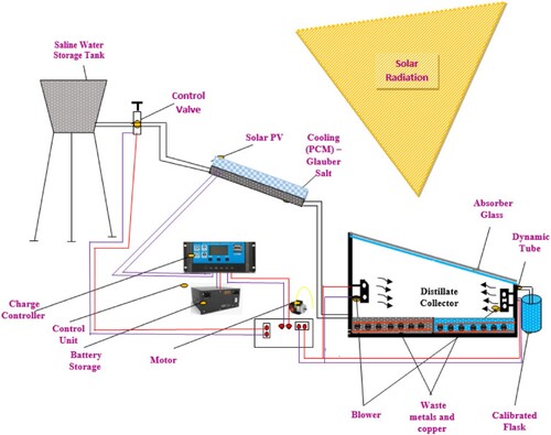
The methods have inclined the solar still through the interior attractive coating via a black coat shined, and the furthermore solar still reservoir has rubbed metals in the lowermost plane which accumulate to the temperature elements. The efficiency of the temperature elements will be functioned through the PV charger supervisor with the assistance of dual blowers placed in the solar still reservoir. The depth of the aquatic range is maintained in the solar still reservoir at 1.5 cm. The utilisation of waste metal to deposit temperature elements, whereas it functions through those temperature elements being converted into water, will be amplified depending on the thermal competence progressively improved in the interior of a solar still reservoir. The blower is operated every 15 minutes or 30 seconds as a purpose to improve evaporation and condensation progression in the solar still compartment. The progression happens between the lowermost plane of solar stills and the topmost plane of waste irons. The condensation of the little droplets of fluid is produced after warm air reaches a cool surface. The evaporation progression enhances the compression amount, respectively growing the distilled invention. So, the water evaporation proportion improved as related through a conservative technique. PV competence is amplified with the help of PCM. The PCM-making proportion is 1:2.5 (water: Glauber salt). The necessary quantity of PCM and the necessary quantity of water are mixed in the correct ratio to formulate a glue nature to permit PCM magnification through 2.4 mm of dense material within the rear plane of the PV. It stimulates worthy thermal parameters and improves the functioning of PV. In investigational proof, the aquatic penetration in the solar still is upheld at 1.5 cm. Here, the investigated data is classified into two types: the primary one is the training data, which is taken by experimental procedures, and the next one is the testing data, which is taken randomly with consideration of various literature. The testing statistics are intended to check the function of ML algorithms. The ratio of training and testing dates is 90:10, 80:20, 70:30, and 60:40, respectively. The experiment of hybrid PV/T solar stills is used to waste metals, with dual blowers as a result of continuous heating of water, and the experiment reading is taken out every 15 minutes in the reproducibility method. The work was completed in favour of continual evaluation, which was carried out hour by hour using the reproducibility method. The evaluation parameters are solar irradiation (Irr), ambient temperature (Ta), glass temperature (Tg), basin temperature (Tb), water temperature (Tw), yield and cumulative yield of solar still, PV panel temperature, PV output power, and power efficiency. The experimental data availed from solar PV is shown in Table 1. The total 41 datasets taken for the evaluation are classified as training and testing data.

Table 1. Comparative analysis of Correlation Values of Cumulative Yield and Output PV.

Parameters	Correlation Values of Cumulative Yield	Correlation Values of Output PV
Time	0.990124	0.020039
Irr	-0.606122	0.723829
Ta	-0.548755	0.719552
Tb	-0.207047	0.944735
Tw	-0.301092	0.914923
Tg	-0.399147	0.868950
Temp-PV	-0.222345	0.933550

3. Methodology

For a given solar PV still dataset, cumulative yield, PV output, and efficiency are the objective values corresponding to the output parameters, and other parameters such as Irr, Ta, Tg, Tb, Tw, and PV temperature are input parameters. LR, RF, XGBR, AdaBR, RR, SVR, EN, and L are various regression methods used in ML techniques. The key factors of evaluation are such things as mean squared error (MSE), mean absolute error (MAE), and root mean squared error (RMSE), R². The methods are skilled with a central processing unit via 8-GB random access memory system models. RMSE, MSE, MAE, and R² score are used to measure the ML regression precision. The functions RMSE, MSE, and MAE are represented as equations (1) to (3). (1) $\mathrm{RMSE}=\sqrt{\sum {\displaystyle \frac{{(y_{\mathrm{pred}}-y_{\mathrm{ref}})}^2}{n}}}$(1) (2) $\mathrm{MSE}={\displaystyle \frac{1}{n}\sum {\displaystyle \frac{{(y_{\mathrm{pred}}-y_{\mathrm{ref}})}^2}{n}}}$(2) (3) $\mathrm{MAE}={\displaystyle \frac{1}{n}\sum |x_i-x|}$(3)

3.1. Regression model

The regression methods applied in this work are a portion of ML. The categories of models acquired as part of the dataset become more evident as well as the ability to construct predictions associated with them. The assistance during submission production includes prediction of the data, analysis of the time series, discovery of the fundamental consequence requirement between the variable quantity, interruption finding, electronic mail filtering, and so on. Furthermore, the regression model in this situation is related to managed learning. This ML technique practices input variable quantity and output variable quantity and, over a procedure, helps map the input variable quantity to the output variable quantity. This data-learning method is beneficial as at the time fresh data is established, the previously mapped performance assists in categorising data effortlessly, and consequently, data can be easily divided or sorted. Here, statistics are used to discover as well as construct an algorithm, and, related to the educated algorithm, statistics are used to forecast; thus, the actual idea creates the essence of every ML categorisation technique. Convenient are three key ideas, approximately which the complete outcomes circle. They are decision trees, boosting, and XGBoost. Individually observe resolve by providing an overall vision of the key ideas they comprise.

Boosting, an ML method, is able to decrease partiality and alteration in the dataset. Boosting assistance towards translating poor performers into good ones: A poor performer classifier is poorly associated with the real classification, while a good performer is better associated. Algorithms that are able to do the above are basically developed while ‘boosting’. Further, most algorithms repeatedly absorb poor classifiers as well as enhance them towards a good one. The additional statistics are subjective; consequently, those statistics are appropriately classified as dropping weight as well as individuals’ misclassified achieving weight. Altogether, in every case, the statistics become reweighted after construction awakens a good apprentice since a poor apprentice is usual. Procedures through the adaptive boosting algorithm are established and suggested. The key dissimilarity among numerous boosting algorithms is the technique of weighting the training data and its assumptions.

XGBoost is mostly considered for speed and efficiency by means of gradient-boosted decision trees. It characterises a method aimed at machine boosting, or in additional disputes relating to machine boosting, primarily prepared through, besides additional engagement via numerous designers. It is an instrument that goes to the Distributed ML Community (DMLC). XGBoost, or Extreme Gradient Boosting, assists in developing each fragment of memory as well as hardware assets in support of tree-boosting models. It provides the advantage of algorithm improvement, alteration of the replica, and being able to be organised in workout environments. XGBoost will be able to achieve the three main gradient boosting methods: gradient boosting, regularised boosting, and stochastic boosting. It, too, permits the accumulation as well as alteration of accepted parameters, and its creation has arisen from supplementary libraries. The algorithm is extremely active in decreasing the workout period as well as delivering optimum usage of memory properties. It is scrubby conscious, can obtain lost standards, supports parallel assembly in a tree structure, and has the exclusive superiority to achieve boosting on additional data previously obtained on the trained replica.

A random-forest classifier is prepared from numerous categorisation trees. The kth classification tree is a classifier signified by an unlabelled input vector and a randomly produced vector through a choice of random specifications of the preparation data for every node. The randomly produced vector of dissimilar categorisation trees in the forest is not associated with everyone, but it is produced with the same allocation algorithm. For unlabelled data, every tree will deliver a forecast or poll in addition to ensuring classification is complete.

3.1.1. Random forest regression

The Random Forest (RF) method produces the selection of a binary tag as a last point, parallel to logistic regression. Random forest regression constructs the decision trees (DT), individually forecasting a dissimilar product through the greatest predominant forecast allocation as the ultimate output. It is accepted misunderstanding that LR approaches build linear performance. RF regression is a real-time controlled learning technique for talking about regression problems. This category of regression is able to combine numerous groups of DT. The ultimate product of this regression technique is obtained as an average of the output of individually combined DT. These energetic DTs are recognised as basic replicas, and their calculations can be noted down. A predominant misunderstanding is that linear regression procedures can only produce linear performance. The random forest design is an active methodology for talking about regression problems. In this category of regression, many groups of DT are able to be joined, and the outcome is described as the mean of the production of individually collective DT. These DTs are mentioned as basic replicas as well as being able to be symbolised through an equation (4(4) $y={\beta }_0+{\beta }_1\mathrm{xory}={\beta }_0+{\beta }_1{X}_1+{\beta }_2{X}_{2.}+\dots ..+{\beta }_n{X}_n$(4) ). (4) $y={\beta }_0+{\beta }_1\mathrm{xory}={\beta }_0+{\beta }_1{X}_1+{\beta }_2{X}_{2.}+\dots ..+{\beta }_n{X}_n$(4)

4. Hyperparameter tuning

In a somewhat ML algorithm, hyperparameters are essential to be prepared before a replica begins the training. Fine-tuning the replica hyperparameters makes the most of the functioning of the model in an authentication grouping. In ML, a hyperparameter is a value of a parameter established prior to starting the learning procedure. On the other side, the values of replica parameters are determined through training the statistics. R replica parameters refer to the weights and constants, which are consequential from the data through the algorithm. Each algorithm has a definite set of hyperparameters; in favour of a sample, for a DT, this is a penetration parameter. Previously, we clarified our hyperparameter tuning method. It is significant to clarify a procedure named ‘cross-validation’, as it is a significant stage in the hyperparameter tuning procedure. Cross-validation (CV) is an algebraic technique that helps assess the precision of ML methods. When the sample is trained, we cannot be convinced in what way it will work on data that have not been previously met. A declaration is required concerning the precision of the forecast function of the replica. The method is to assess the function of an ML model, hidden data is required for the test.

Related to the replica function taking place in the hidden data, we are able to identify whether the replica is underneath fitting, overfitting, or well-sweeping. Cross-validation is an extremely generous method to examine in what way an ML model is better while the data in the model are restricted. In order to achieve cross-validation, a division of the data must be set apart for testing and authorising; this division will not be used to train the replica but is nevertheless somewhat protected for future usage. K-Fold is the greatest communal method of cross-validation, and in addition to it, the cross-validation method that we used to authenticate our replica is shown in Figure 2.

Figure 2. K-Fold cross-validation.

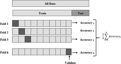
In K-Fold cross-validation, the K points out the number of folds or segments into which an assumed dataset is divided. One fold is reserved as an authenticating set, and the ML replica is trained by means of the enduring K-1 folds. Individual folds of the K-folds are used as an authenticating set at several points by means of K scores (precision) assumed as an outcome. Lastly, we average the replica in contradiction to each of the folds individually to acquire an ultimate score for the replica, as shown in Figure 2.

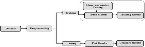
The significance of hyperparameters’ falsehood is their capability to straight-regulate the performance of the training algorithm. Selecting suitable hyperparameters plays a very significant role in the function of the replica being trained. It is significant to have three sets on which the data are separated, i.e. a training, testing, and validation set, when the defaulting parameter is changed in order to acquire the essential precision and, consequently, to avoid data leakages. Therefore, hyperparameter tuning can be easily definite while the procedure of discovering the greatest hyperparameter standards of a learning algorithm so as to harvest the greatest replica. The method of discovering the greatest hyperparameter values by means of respect for a particular dataset has conventionally been achieved physically. In the direction of setting these values, investigators regularly rely on their previous understanding of training these ML algorithms in resolving similar difficulties. The difficulties are that the finest background for hyperparameters used to resolve one issue might not remain the finest background on behalf of an additional one, as these values will vary through dissimilar datasets. Therefore, it is problematic to describe the hyperparameter values related to the earlier understanding. A further automatic, directed technique is required to discover substitute formations of the ML model under study. Generally, hyperparameter optimisation algorithms include grid search, random search, and Bayesian optimisation. In this effort, grid search is recognised as a hyperparameter optimisation for numerous ML methods, as shown in Figure 3.

Figure 3. Hyperparameter based learning algorithm.

4.1. Grid search

The ultimate spontaneous conventional method for functioning hyperparameter optimisation is grid search. It produces a Cartesian invention for every potential grouping of hyperparameters. Grid Search sequences the ML algorithm for every grouping of hyperparameters; this method must be directed through a function metric, characteristically estimated by means of the ‘cross-validation’ method taking place in the training set. This validation method guarantees that the trained replica finds the greatest number of designs in the dataset. Grid search is apparently the greatest straight-on hyperparameter tuning technique. With this method, we construct a grid through each potential grouping of all the hyperparameter standards delivered, compute the score of each replica during instruction toward estimating it, and then choose the replica that offers the greatest outcomes. To execute Grid Search, one chooses a determinate set of realistic values for each hyperparameter; the Grid Search algorithm formerly trains the replica through every grouping of the hyperparameters inside the Cartesian creation.

The function of grouping is estimated to take place during a held-out authentication set or throughout interior cross-validation scheduled for the training set. Lastly, the grid search algorithm produces the set that accomplishes the uppermost function in the evaluation process. The greatest set of hyperparameter values selected in the grid search is the next step in the real replica. Grid Search assures the discovery of the greatest hyperparameters. If k parameters through n separate values are tested, the difficulty of grid search is predictable to produce exponentially at a rate of O (NK).

5. Results and discussion

The proposed method uses a hybrid PV/T still system dataset and analyzes the polarity of positive or negative data; ineffective data are omitted. A concise argument is agreed upon in the subsequent subsections in the direction of clarifying the ladder assumed through our PVT still method within regulation toward the completely assembled. Eight managed ML methods are discussed, such as LR, RF, XGBR, AdaBR, RR, SVR, EN, and L. Throughout this method; the ML regression was trained to predict the output as the cumulative yield of freshwater, PV output, and efficiency. In this work, time, Irr, Ta, Tg, Tb, Tw, and PV temperature are the input parameters, and cumulative yield, PV output power, and power efficiency are the output variables.

5.1. Modelling of solar PV still by standard hyperparameters

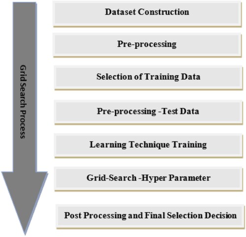
Primary, the accuracy of every ML replica in predicting the yield of freshwater by the standard values of the hyperparameters Totally 41 datasets have been analyzed; here, thus, datasets classify training and testing with the following ratios: 90:10, 80:20, 70:30, and 60:40, respectively. Here, we used the standard values particular to the Python scikit-study documentation package. Google Colab helps investigate datasets by initially loading the dataset and investigating its time, irradiation, heat, and parameter categories. After that, analyze every characteristic intended for abnormality. An illustration of the Grid search parameter tuning approach is presented in Figure 4.

Figure 4. Grid search parameter tuning.

5.1.1. Data set construction and preprocessing data

Initially, all datasets were pre-processed by shaping, and it was found that except for the column ‘Irr, all column datatypes were float 64. The data has seven quantitative input variables and three quantitative output variables: cumulative yield of freshwater, PV output, and efficiency. The analytical ML methods intended for water yield and PV output are exhibited as regression replicas. The data types are float 64 and int 64, the storage handling is 7.1 KB, the date profile is (41, 10), and the date dimension is 410. There are completely 10 features, and the datatypes were previously numeric. Therefore, no alteration of datatypes was necessary. The complete features are linear; readily available are excellent numbers of data values for every feature. Here, there are no null values in any of the features, so null value handling is not necessary. The completeness of the features is significant; it does not require dropping any of the features more than the cumulative yield of freshwater, PV output, and efficiency, which are the objective variables. The values of the features are in dissimilar units, so they need to be transformed to the general type with pre-processors. There might be a few outliers in the data, so consider doing a few outlier processes. Next, check the duplicates and drop the duplicates by predicting outliers. Also, it was found that there was no missing value in the data. In the Outliers analysis, the irr’ column has an outlier, which demands an extra methodical revision earlier than the proper outliers, and altering the outliers will put pressure on data excellence. The parameters of time, Irr, Ta, Tg, Tb, and Tw have a higher influence on the target variable of cumulative yield, and PV temperature has a higher influence on the output variables of PV power and efficiency. Figure 5 (a-c-e-g-i-k-m) represents the individual importance of each parameter with its respective cumulative yield.

Figure 5. Outliers of all parameters.

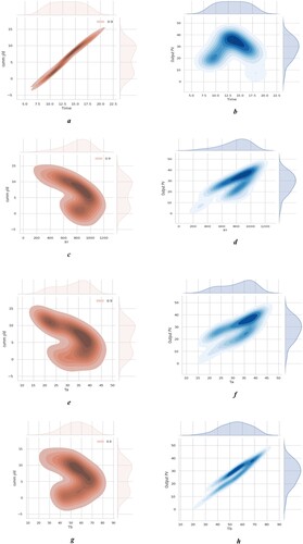
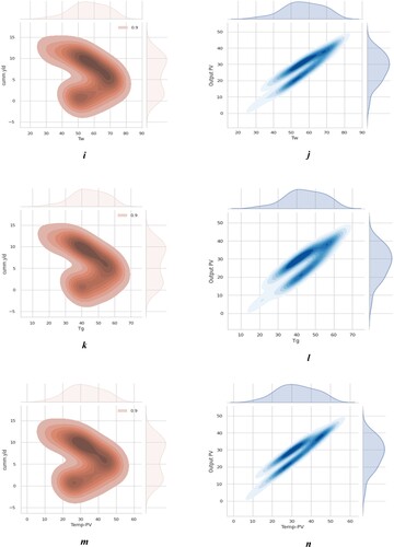
All figures reflected the cumulative yield, which depends on varying particular parameters. Generally, the yield of the water depends on the thermal characteristics of the solar still, such as Ta, Tg, Tb, and Tw. When it increases the thermal characteristics as well as enhances the fresh water yield. The plot shows that all the thermal characteristics gradually increase from 8.30 a.m. to 1.00 p.m., then gradually decrease up to 6.30 p.m. The time of 12.00 am to 1.00 pm has the highest thermal performance, as represented in the dark-orange colour field. The peak value of time at 1.00 p.m. is Irr-1030, Ta-40.4°C, Tg-72.6°C, Tb-73.1°C, and Tw-60.2°C. The parameter Temp PV is not considered in the cumulative yield analysis. At the same time, the time of 12.00 am to 1.00 pm has the highest thermal performance, particularly panel temperature, which is represented in dark blue (Figure 5 (b-d-f-h-j-l-n) colour field). When the panel temperature (Temp PV) increases as well as decreases, the performance of the panel, power and efficiency are reduced. But here, using PCM to stimulate a worthy thermal parameter and improve the functioning of PV, The peak value of time at 1.00 p.m. is Irr-1030, temp PV-48.9, output PV-41.6 watts, and efficiency 11.65%. The parameters Ta, Tg, Tb, and Tw are not considered in the output PV analysis.

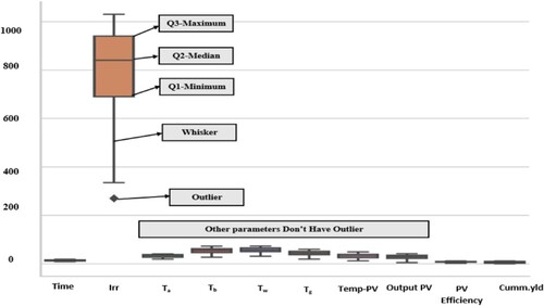
Figure 6 box plot represents all the input variables and output variables with respective analyses of quartiles 1, 2, and 3 and outliers. Here, the input parameters of irradiation have quartile values of Q1-1017.5, Q2-1020, and Q3-1370, and the lower and higher outlier values are 488.75 and 1898.75, respectively. So, the irradiation has a lower outlier value of 270 W/m2, which is represented in the figure. At the same time, except for irradiation and analysis, all other input and output variables do not have outliers.

Figure 6. Relationship Between all Input variables with cumulative yield and PV output.

5.1.2. Variables correlation

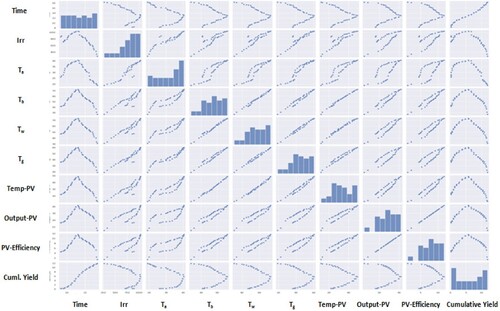
Multiple pairwise bivariate distributions in datasets describes all input and output parameters with respect to one another, such as cumulative yield, PV output and efficiency, Irr, Ta, Tg, Tb, Tw, and PV temperature. The Table 3 shows that with the correct correlation line cumulative yield with thermal characteristics Ta, Tg, Tb, and Tw, the performance indexes are highly efficient. Otherwise, the not-perfect correlation line indicates that the temperature PV increases correspondingly decreases the performance of solar PV output.

Figure 7 indicates each individual input with respect to the same input variable; it is a histogram. For each input with respect to all other input variables, an example of irradiation with respect to all other input variables is represented in the figure. (1). Irradiation with Time: In the morning to afternoon, depending on sunlight, the irradiation values increase; after that, the afternoon to evening irradiation decreases. (2). Irradiation with respect to irradiation: make a histogram. (3). Irradiation with respect to T_a, T_b, T_w, Tw, and T_g: It’s the various input temperatures that also increase from morning to afternoon and decrease afterwards. 4. At the same time, irradiation with respect to temperature of PV, output of PV, and cumulative yield of solar still also increases from morning to afternoon and decreases afterwards. When the input variable increases with the respective other input variable increases, the system is positively correlated, and when the input variable increases with the respective other input variable decreases, the system is negatively correlated. In the multivariable system, the analysis values are between +1 and -1. As a result, various types of multivariate correlation graphs make it simple to determine which algorithm is best.

Figure 7. Pairplot of all input and output variables.

Table 1 shows comparative analysis of Correlation Values of Cumulative Yield and Output PV with input features such as time, IRR, Ta, Tb, Tw, Tg, and temperature PV with respect to cumulative yield and output PV. It shows a negative coefficient of ‘irr’ and thermal characteristics (Ta, Tb, Tw, Tg) that have a high impact on the cumulative yield of freshwater, which means they enhance the yield. Next, the positive coefficient of panel temperature (Temp PV) has a high impact on output PV, which means reduced output power. The X-axis input variables are Time, Irr, Ta, Tb, Tw, Tg, and temperature PV, and the Y-axis are cumulative yield and output PV. The figure represents the respective input variable, which is to produce positive and negative correlation coefficients in cumulative yield and output power, respectively. The positive coefficient represents that an increase in the input variable correspondingly increases the output cumulative yield and output power. Examples: time with respect to both yield(0.990124) and power have positive correlation (0.020039) values, and Irr (0.723829), Ta (0.719552), Tb (0.944735), Tw (0.914923), Tg (0.868950), and temperature PV (0.933550) with respect to increase the output power. The negative coefficient represents that an increase in the input variable correspondingly decreases the output cumulative yield and output power. Examples: Irr, Ta, Ta, Tb, Tw, Tg, and temperature PV with respect to decreasing the cumulative yield.

5.1.3. Performance matrices

Table 2 represents the performance matrices of the regression models with various testing and training data sets like 90:10 (size 0.1), 80:20 (size 0.2), 70:30 (size 0.3), and 60:40 (size 0.4). From the table, 60% of training and 40% of data sets provide good performance matrices in the target variable of cumulative yield, and 90% of training and 10% of data sets provide good performance matrices in the target variable of output PV. In all the cases, the random forest tree regression model shows a higher r² score and minimum errors in cumulative yield, and the tuned SVR regression model shows a higher r² score and minimum errors in output PV. From the Table 2, it is found that the Random Forest Tree (RF) and Tuned SVR outperformed the other models, such as the LR, XGBR, AdaBR, RR, EN, and L regressions.

Table 2. Experimental dataset.

S.No	Time of day	Irr (W/m^2)	Ta (°C)	Tb (°C)	Tw (°C)	Tg (°C)	Temp-PV (°C)	Output PV (Watts)	PV Efficiency (%)	Mewg (Kg)	cumm.yld (Kg)
1.	8.30	860	26	41.4	47	36	22.1	16.1	4.51	0.2841478	0.28415
2.	8.45	890	27	41.6	47.4	36.5	22.8	16.6	4.65	0.2864775	0.28648
3.	9.00	710	28	42.8	48	37.2	24	17.4	4.87	0.2914140	0.29141
4.	9.15	730	30	43.6	48.8	38.7	24.5	18.0	5.04	0.2803350	0.28033
5.	9.30	750	32	44.3	49.9	39	24.9	18.4	5.15	0.3207881	0.6122
6.	9.45	765	33.5	47.1	51.4	41.2	26.1	19.2	5.38	0.3184146	0.59875
7.	10.00	790	35	52.5	54.5	43.5	29	21.5	6.02	0.3972232	1.00943
8.	10.15	840	36	53.5	55.6	44.7	29.8	22.6	6.33	0.4124369	1.01119
9.	10.30	860	36.5	55.3	57.6	47.1	32.4	24.7	6.92	0.4309438	1.44037
10.	10.45	900	37	57.1	59.2	48.9	34.1	26.2	7.34	0.4513025	1.46249
11.	11.00	940	37.5	58.6	61.6	50.1	35.6	27.7	7.76	0.5654184	2.00579
12.	11.15	945	38	59.9	63	51.6	37.1	28.9	8.10	0.5935408	2.05603
13.	11.30	955	38.5	62	65.1	52.1	38.7	29.8	8.35	0.7492627	2.75505
14.	11.45	970	38.8	64.5	67.4	54.5	40.5	32.5	9.10	0.8163017	2.87233
15.	12.00	1000	39.1	67.7	69.9	56	43.8	35.4	9.92	0.9805911	3.73564
16.	12.15	1005	39.3	68.5	70.6	57.1	44.8	36.7	10.28	0.9767346	3.84907
17.	12.30	1015	39.5	70.3	71.5	58.3	46	39.3	11.01	0.9876503	4.72329
18.	12.45	1020	39.8	71.5	72	59.4	47.4	39.7	11.12	0.9565526	4.80562
19.	13.00	1030	40.4	72.6	73.1	60.2	48.9	41.6	11.65	1.0257495	5.74904
20.	13.15	1025	40.2	71.4	72.2	58.8	47.6	40.3	11.29	1.0326124	5.83823
21.	13.30	1020	40	69.3	70	56.4	45.4	38.8	10.87	0.9612636	6.71030
22.	13.45	920	38	67.1	68.1	54.3	43.8	37.0	10.36	0.9045153	6.74275
23.	14.00	890	37.2	64.6	65.4	51.8	41.2	36.4	10.20	0.7970183	7.50732
24.	14.15	870	36.4	62.2	63.4	49.1	38.9	35.8	10.03	0.7744147	7.51716
25.	14.30	855	35	61	62.3	48.3	37.7	34.6	9.69	0.7228301	8.23015
26.	14.45	840	34.5	59.9	61.8	47.7	36.6	33.9	9.50	0.7132056	8.23037
27.	15.00	835	32.5	57.3	59	45	34.4	33.0	9.24	0.6283268	8.85848
28.	15.15	800	32	56.1	58	44	33.4	32.5	9.10	0.6018805	8.83225
29.	15.30	765	31	55.3	57	43	32.12	31.4	8.80	0.5763982	9.43488
30.	15.45	735	30.5	54.4	55.8	41.7	31.8	30.8	8.63	0.5512044	9.38345
31.	16.00	690	29.8	53.1	54	40.3	30.2	29.9	8.38	0.4939342	9.92881
32.	16.15	655	27	52.3	53.3	39.9	29.8	28.8	8.07	0.4676863	9.85114
33.	16.30	625	24	51	52	38.1	28.8	28.1	7.87	0.4589385	10.3877
34.	16.45	610	23.5	50	51	37.2	27.1	27.0	7.56	0.4354638	10.2866
35.	17.00	600	23	48	50.1	36.5	26.1	26.4	7.39	0.4117222	10.7994
36.	17.15	565	22.5	46.5	47.5	34.4	24.2	24.9	6.97	0.3514543	10.6380
37	17.30	510	22	43	45	33	23	24.1	6.75	0.2849831	11.0844
38	17.45	470	21	40	42.1	30.3	20.6	22.4	6.27	0.2442438	11.3287
39	18.00	420	20.5	37	40	28	17.7	19.0	5.32	0.2249948	11.5536
40	18.15	335	20	31	33.6	22.7	13.5	08.5	2.38	0.1482012	11.7019
41	18.30	270	19	27	31.1	19.1	12	05.0	1.40	0.1447753	11.8466

Table 3 represent the models RMSE for each regression algorithm and the RMSE score of each regression algorithm, the RMSE is the calculated difference between the actual value and the predicted value. RMSE is one of the methods used to predict the accuracy of regression models. Table 2 shows the calculated RMSE values in training and testing data for various regression algorithms. The RMSE values are low, but the models have high accuracy. The calculation of RMSE values is used to identify which model is highly suitable for system operation. The training and testing data is 60:40 (size 0.4), and the tuned random forest model's RMSE value is 0.2583. Table represent the models R² for each regression algorithm and the R² score of each regression algorithm, The R² Values are close to +1 or -1. R² is one of the methods used to predict the accuracy of regression models. Table 2 represents the calculated R² values in training and testing data for various regression algorithms. The high value of R², the relationship between two variables is high. The training and testing data is 60:40 (size 0.4), and the tuned random forest model's R² value is 0.9952.

Table 3. Comparison of regression models with various training sets.

Model	Cumulative Water Yield				Output PV
	MAE	MSE	r^2 Score	RMSE	MAE	MSE	r^2 Score	RMSE
Training and Testing data 90:10 (Size 0.1)
Tuned Random Forest Regressor	0.2605	0.0850	0.9922	0.2916	2.7787	9.1984	0.7681	3.0329
Random Forest Regressor	0.2992	0.1220	0.9889	0.3492	2.3848	6.7291	0.8303	2.5940
Tuned XGB Regressor	0.3216	0.2067	0.9811	0.4547	2.0319	5.0766	0.8720	2.2531
XGB Regressor	0.3165	0.2064	0.9811	0.4543	1.7809	4.0537	0.8978	2.0134
Tuned Ada Boost Regressor	0.3994	0.2319	0.9788	0.4816	2.9146	10.3245	0.7397	3.2132
Ada Boost Regressor	0.4199	0.2851	0.9739	0.5339	2.8193	8.4178	0.7878	2.9014
Tuned Ridge	0.4474	0.2759	0.9748	0.5253	1.2537	1.8442	0.9535	1.3580
Ridge	0.5696	0.4322	0.9605	0.6574	1.2537	1.8442	0.9535	1.3580
Tuned Lasso	0.5223	0.3448	0.9685	0.5872	1.3905	1.9897	0.9498	1.4106
Lasso	1.2956	1.7052	0.8442	1.3058	2.0403	4.4103	0.8888	2.1001
Tuned SVR	0.3232	0.1110	0.9899	0.3331	0.4128	0.2587	0.9935	0.5087
SVR	1.3819	2.0360	0.8139	1.4269	1.9696	5.4390	0.8629	2.3322
Tuned Elastic Net	0.4155	0.2448	0.9776	0.4948	1.2749	2.0992	0.9471	1.4489
ElasticNet	1.8819	3.7700	0.6554	1.9417	2.3583	5.8783	0.8518	2.4245
Linear Regression	0.3936	0.2319	0.9788	0.4816	1.2581	2.2041	0.9444	1.4846
Training and Testing data 80:20 (Size 0.2)
Tuned Random Forest Regressor	0.2573	0.0821	0.9949	0.2865	4.6686	47.1641	0.6491	6.8676
Random Forest Regressor	0.3001	0.1064	0.9933	0.3261	4.7250	50.7312	0.6226	7.1226
Tuned XGB Regressor	0.3392	0.2164	0.9864	0.4652	3.9895	36.7071	0.7269	6.0586
XGB Regressor	0.3359	0.2158	0.9865	0.4646	3.8474	36.6093	0.7276	6.0506
Tuned Ada Boost Regressor	0.4895	0.3448	0.9784	0.5872	4.5679	45.5417	0.6612	6.7485
Ada Boost Regressor	0.4204	0.2445	0.9847	0.4945	4.5393	46.3675	0.6550	6.8094
Tuned Ridge	0.5043	0.5296	0.9668	0.7278	2.4808	19.2215	0.8570	4.3842
Ridge	0.4026	0.2999	0.9812	0.5476	2.5265	16.9890	0.8736	4.1218
Tuned Lasso	0.5270	0.5893	0.9630	0.7677	2.7292	27.1233	0.7982	5.2080
Lasso	1.0511	1.2586	0.9211	1.1219	3.8296	30.2297	0.7751	5.4982
Tuned Elastic Net	0.4949	0.5146	0.9677	0.7173	2.6520	25.3460	0.8114	5.0345
ElasticNet	1.5670	2.7090	0.8301	1.6459	4.1450	29.9545	0.7771	5.4731
Tuned SVR	0.2963	0.1162	0.9927	0.3408	2.1433	15.2763	0.8864	3.9085
SVR	1.6582	4.9144	0.6918	2.2169	6.3520	87.9708	0.3455	9.3793
Linear Regression	0.5672	0.6752	0.9577	0.8217	2.7434	27.4135	0.7961	5.2358
Training and Testing data 70:30 (Size 0.3)
Tuned Random Forest Regressor	0.2685	0.0989	0.9933	0.3145	4.1774	36.9744	0.6725	6.0807
Random Forest Regressor	0.2878	0.1113	0.9925	0.3337	4.1860	37.6088	0.6669	6.1326
Tuned XGB Regressor	0.3507	0.2366	0.9840	0.4864	3.4255	28.0906	0.7512	5.3001
XGB Regressor	0.3494	0.2373	0.9840	0.4871	3.3326	27.7576	0.7541	5.2685
Tuned Ada Boost Regressor	0.4709	0.3100	0.9791	0.5568	4.4339	38.1265	0.6623	6.1747
Ada Boost Regressor	0.3875	0.2524	0.9830	0.5024	4.2715	35.1012	0.6891	5.9246
Tuned Ridge	0.3787	0.3525	0.9762	0.5937	2.0281	17.1582	0.8480	4.1422
Ridge	0.4431	0.3131	0.9789	0.5595	2.1474	12.5238	0.8891	3.5389
Tuned Lasso	0.4011	0.4053	0.9727	0.6366	2.0780	18.2997	0.8379	4.2778
Lasso	1.0285	1.2485	0.9158	1.1174	3.2429	19.3405	0.8287	4.3978
Tuned Elastic Net	0.3908	0.3796	0.9744	0.6161	2.0455	17.3229	0.8466	4.1621
ElasticNet	1.4683	2.5902	0.8253	1.6094	3.7048	22.9995	0.7963	4.7958
Tuned SVR	0.4044	0.3622	0.9756	0.6018	1.5238	11.6615	0.8967	3.4149
SVR	1.6138	3.7477	0.7472	1.9359	5.5945	67.2217	0.4046	8.1989
Linear Regression	0.4202	0.4505	0.9696	0.6712	2.0604	18.3911	0.8371	4.2885
Training and Testing data 60:40 (Size 0.4)
Tuned Random Forest Regressor	0.2284	0.0667	0.9952	0.2583	3.5529	29.7120	0.6996	5.4509
Random Forest Regressor	0.2704	0.1158	0.9917	0.3403	3.5605	29.8536	0.6981	5.4638
Tuned XGB Regressor	0.5319	0.3868	0.9724	0.6220	2.5967	20.2494	0.7952	4.4999
XGB Regressor	0.4381	0.3129	0.9776	0.5594	2.6461	20.7713	0.7900	4.5576
Tuned Ada Boost Regressor	0.4461	0.3284	0.9765	0.5731	3.5087	28.1947	0.7149	5.3099
Ada Boost Regressor	0.4450	0.3290	0.9765	0.5736	3.6262	29.4041	0.7027	5.4226
Tuned Ridge	0.3225	0.2725	0.9805	0.5221	1.7175	14.2888	0.8555	3.7801
Ridge	0.5026	0.3382	0.9758	0.5816	1.8325	10.0357	0.8985	3.1679
Tuned Lasso	0.3471	0.3169	0.9774	0.5630	1.7759	15.4661	0.8436	3.9327
Lasso	1.0273	1.2612	0.9099	1.1230	2.7827	15.1217	0.8471	3.8887
Tuned Elastic Net	0.3165	0.2582	0.9816	0.5081	1.7276	14.3778	0.8546	3.7918
ElasticNet	1.4088	2.4431	0.8254	1.5630	3.2605	18.6045	0.8119	4.3133
Tuned SVR	0.2574	0.1040	0.9926	0.3224	1.2715	7.3998	0.9252	2.7203
SVR	1.8244	4.7955	0.6573	2.1899	5.5162	59.5702	0.3976	7.7182
Linear Regression	0.3659	0.3647	0.9739	0.6039	1.7872	15.6550	0.8417	3.9566

6. Conclusion

In this study, the prediction of machine learning models for hybrid PV/T solar still was established based on LR, RF, XGBR, AdaBR, RR, SVR, EN, and L regression models. The regression model precision of every ML model was optimised by the use of grid search CV tuning to get superior accuracy. Afterwards, acquire, by the model's standards, the values of the hyperparameters. The proposed work, Grid Search hyperparameter tuning methods, is obtainable, and these methods are used towards the function of the hyperparameter tuning of eight ML algorithms in order to analyze fresh water. Our outcomes describe the following:

• The RF and Tuned Random Forest regression propose the greatest accuracy together earlier and after hyperparameter tuning in cumulative yield, with the highest r2score of 0.9952 obtained when using Grid search CV for the test size 0.4 (60:40 ratio of training and testing).

• The RMSE value of RF is reduced to 0.2583. The SVR and Tuned SVR regressions propose the greatest accuracy together earlier and after hyperparameter tuning in output PV, with the highest score of 0.9935obtained when using Grid Search CV for the test size of 0.1 (90:10 ratio of training and testing).

• The RMSE value of SVR is reduced to 0.5087. Meanwhile, tuned XGBR, AdaBR, RR, EN, and L regression models dramatically enhanced the grid search score. The linear regression does not have the tuned grid search scores.

• The proposed work performance matrix analysis is to identify which type of algorithm gives the best accuracy in terms of solar PV electrical efficacy and solar thermal efficiency.

• Thus, the RF and tuned random forest regression models are suggested for effective modelling and characterising the power production and water productivity of hybrid PVT.

• This work proves that it depends on modelling RF and tuned random forest regression methods to save time, effective production of solar PV power, and solar yield and increase the financial benefits.

• The correlation obtained from the regression model is accessible mathematically for predicting power production and water yield in terms of the eight parameters mentioned.

• In the future, the effect of different natural materials for solar PV cooling and solar still heating will enhance the power output and thermal efficiency.

Disclosure statement

No potential conflict of interest was reported by the author(s).

Data availability statement

The datasets generated during and/or analysed during the current study are not publicly available but are available from the corresponding author on reasonable request.

References

- Abdulsahib, Ghaida Muttashar, Dhana Sekaran Selvaraj, A. Manikandan, Satheesh Kumar Palanisamy, Mueen Uddin, Osamah Ibrahim Khalaf, Maha Abdelhaq, and Raed Alsaqour. 2023. “Reverse Polarity Optical Orthogonal Frequency Division Multiplexing for High-Speed Visible Light Communications System.” Egyptian Informatics Journal 24 (4): 100407. https://doi.org/10.1016/j.eij.2023.100407.
- Abou Houran, Mohamad, Syed M. Salman Bukhari, Muhammad Hamza Zafar, Majad Mansoor, and Wenjie Chen. 2023. “COA-CNN-LSTM: Coati Optimization Algorithm-Based Hybrid Deep Learning Model for PV/Wind Power Forecasting in Smart Grid Applications.” Applied Energy 349: 121638. https://doi.org/10.1016/j.apenergy.2023.121638.
- Abujazar, Mohammed S. S., Suja Fatihah, Ibrahim Anwar Ibrahim, A. E. Kabeel, and Suraya Sharil. 2018. “Productivity Modelling of a Developed Inclined Stepped Solar Still System Based on Actual Performance and Using a Cascaded Forward Neural Network Model.” Journal of Cleaner Production 170: 147–159. https://doi.org/10.1016/j.jclepro.2017.09.092.
- Ağbulut, Ümit, Ali Gürel, and Yunus Biçen. 2021. “Prediction of Daily Global Solar Radiation Using Different Machine Learning Algorithms: Evaluation and Comparison.” Renewable and Sustainable Energy Reviews 135: 110114. https://doi.org/10.1016/j.rser.2020.110114.
- Ahmad, Ashfaque, Harish Ghritlahre, and Purvi Chandrakar. 2020. “Implementation of ANN Technique for Performance Prediction of Solar Thermal Systems: A Comprehensive Review.” Trends in Renewable Energy 6 (1): 12–36. https://doi.org/10.17737/tre.2020.6.1.00110.
- Alyu, A. B., A. O. Salau, B. Khan, and J. N. Eneh. 2023. “Hybrid GWO-PSO Based Optimal Placement and Sizing of Multiple PV-DG Units for Power Loss Reduction and Voltage Profile Improvement.” Scientific Reports 13 (1): 6903. https://doi.org/10.1038/s41598-023-34057-3.
- Bahiraei, M., S. Nazari, H. Moayedi, and H. Safarzadeh. 2020. “Using Neural Network Optimized by Imperialist Competition Method and Genetic Algorithm to Predict Water Productivity of a Nanofluid-Based Solar Still Equipped with Thermoelectric Modules.” Powder Technology, https://doi.org/10.1016/j.powtec.2020.02.055.
- Bamisile, Olusola, Dongsheng Cai, Ariyo Oluwasanmi, Chukwuebuka Ejiyi, Chiagoziem Ukwuoma, Oluwasegun Ojo, M. Bn Mukhtar, and Qi Huang. 2022. “Comprehensive Assessment, Review, and Comparison of AI Models for Solar Irradiance Prediction Based on Different Time/Estimation Intervals.” Scientific Reports 12. https://doi.org/10.1038/s41598-022-13652-w.
- Chandan, K., K. V. Nagaraja, Fehmi Gamaoun, T. V. Smitha, N. Neelima, Umair Khan, and Ahmed M Hassan. 2024. “Improving Flow Efficiency in Micro and Mini-Channels with Offset Strip Fins: A Stacking Ensemble Technique for Accurate Friction Factor Prediction in Steady Periodically Developed Flow.” Case Studies in Thermal Engineering 56: 104232. https://doi.org/10.1016/j.csite.2024.104232.
- Chauhan, Rishika, Shefali Sharma, Rahul Pachauri, Pankaj Dumka, and Dhananjay R Mishra. 2020. “Experimental and Theoretical Evaluation of Thermophysical Properties for Moist air Within Solar Still by Using Different Algorithms of Artificial Neural Network.” Journal of Energy Storage 30: 101408. https://doi.org/10.1016/j.est.2020.101408.
- Chinnamayan, Vennila, Anita Titus, T. Sudha, U. Sreenivasulu, N. Reddy, K. Jamal, Dayadi Lakshmaiah, P. Jagadeesh, and Assefa Belay. 2022. “Forecasting Solar Energy Production Using Machine Learning.” International Journal of Photoenergy 2022: 1–7. https://doi.org/10.1155/2022/7797488.
- Elgeldawi, E., A. Sayed, A. R. Galal, and A. M. Zaki. 2021. “Hyperparameter Tuning for Machine Learning Algorithms Used for Arabic Sentiment Analysis.” Informatics 8: 79. https://doi.org/10.3390/informatics8040079.
- Elsayed Abd Elaziz, Mohamed, Emad El-Said, Ammar Elsheikh, and Gamal Abdelaziz. 2022. “Performance Prediction of Solar Still with a High-Frequency Ultrasound Waves Atomizer Using Random Vector Functional Link/Heap-Based Optimizer.” Advances in Engineering Software 170: 103142. https://doi.org/10.1016/j.advengsoft.2022.103142.
- Elsheikh, Ammar H., Vikrant P. Katekar, Otto L. Muskens, Sandip S. Deshmukh, Mohamed Abd Elaziz, and Sherif M Dabour. 2021. “Utilization of LSTM Neural Network for Water Production Forecasting of a Stepped Solar Still with a Corrugated Absorber Plate.” Process Safety and Environmental Protection 148: 273–282. https://doi.org/10.1016/j.psep.2020.09.068.
- Essa, F. A., Mohamed Abd Elaziz, and Ammar H Elsheikh. 2020. “An Enhanced Productivity Prediction Model of Active Solar Still Using Artificial Neural Network and Harris Hawks Optimizer.” Applied Thermal Engineering 170: 115020. https://doi.org/10.1016/j.applthermaleng.2020.115020.
- Faremi, A. A., O. Olubosede, A. O. Salau, S. O. Adigbo, P. A. Olubambi, and E. Lawan. 2023. “Variability of Temperature on the Electrical Properties of Heterostructured CIS/Cds Through SCAPS Simulation for Photovoltaic Applications.” Materials for Renewable and Sustainable Energy 12 (3): 235–246. https://doi.org/10.1007/s40243-023-00244-5.
- Gaboitaolelwe, J., A. M. Zungeru, A. Yahya, C. K. Lebekwe, D. N. Vinod, and A. O. Salau. 2023. “Machine Learning Based Solar Photovoltaic Power Forecasting: A Review and Comparison.” IEEE Access 11: 40820–40845. https://doi.org/10.1109/ACCESS.2023.3270041.
- Hailu, E. A., A. J. Godebo, G. L. S. Rao, A. O. Salau, T. F. Agajie, Y. A. Awoke, and T. M. Anteneh. 2021. “Assessment of Solar Resource Potential for Photovoltaic Applications in East Gojjam Zone, Ethiopia. Lecture Notes of the Institute for Computer Sciences.” Social Informatics and Telecommunications Engineering 384. Springer, Cham. https://doi.org/10.1007/978-3-030-80621-7_28.
- Jebril, Iqbal, P. Dhanaraj, Ghaida Muttashar Abdulsahib, Satheesh Kumar Palanisamy, T. Prabhu, and Osamah Ibrahim Khalaf. 2022. “Analysis of Electrically Couple SRR EBG Structure for Sub 6 GHz Wireless Applications.” Advances in Decision Sciences, Asia University, Taiwan 26 (Special): 102–123.
- Kandasamy, Anguraj, Saravanakumar Rengarasu, Praveen Kitti Burri, Satheesh kumar Palanisamy, K. Kavin Kumar, Aruna Devi Baladhandapani, and Samson Alemayehu Mamo. 2022. “Defected Circular-Cross Stub Copper Metal Printed Pentaband Antenna.” Advances in Materials Science and Engineering 2022: Article ID 6009092, 10. https://doi.org/10.1155/2022/6009092.
- Kumar, Satheesh, and T. Balakumaran. 2021. “Modeling and Simulation of Dual Layered U-Slot Multiband Microstrip Patch Antenna for Wireless Applications.” Nanoscale Reports 4 (1): 15–18. https://doi.org/10.26524/nr.4.3.
- Mashaly, Ahmed, and Prof Alazba. 2019. “Assessing the Accuracy of ANN, ANFIS, and MR Techniques in Forecasting Productivity of an Inclined Passive Solar Still in a hot, Arid Environment.” Water SA 45: 239. https://doi.org/10.4314/wsa.v45i2.11.
- Mitra, I., D. Heinemann, A. Ramanan, M. Kaur, S. K. Sharma, and S. K. Tripathy. 2022. “Short-term PV Power Forecasting in India: Recent Developments and Policy Analysis.” International Journal of Energy and Environmental Engineering 13 (2): 515–540. https://doi.org/10.1007/s40095-021-00468-z.
- Mukti, P., L. Lusiana, D. Titisari, and S. Palanisamy. 2023. “Performance Analysis of Twelve Lead ECG Based on Delivery Distance Using Bluetooth Communication.” Journal of Electronics, Electromedical Engineering, and Medical Informatics 5 (1): 46–52. https://doi.org/10.35882/jeeemi.v5i1.275
- Nazari, Saeed, Mehdi Bahiraei, Hossein Moayedi, and Habibollah Safarzadeh. 2020. “A Proper Model to Predict Energy Efficiency, Exergy Efficiency, and Water Productivity of a Solar Still via Optimized Neural Network.” Journal of Cleaner Production, 123232. https://doi.org/10.1016/j.jclepro.2020.123232.
- Nazari, Mohammad, Mohamed Salem, Ibrahim Mahariq, Khaled Younes, and Bashar Maqableh. 2021. “Utilization of Data-Driven Methods in Solar Desalination Systems: A Comprehensive Review.” Frontiers in Energy Research 9: 1–11. https://doi.org/10.3389/fenrg.2021.742615.
- Orelusi, A. N., V. A. Owoeye, J. B. Dada, A. O. Salau, H. O. Boyo, and S. A. Adewinbi. 2023. “Investigation of Microstructure and Optical Characteristics of Ti-Doped ZnO Thin Films as an Effective Solar Collector in Photovoltaic Solar Cell Applications Using Digitally Controlled Spray Pyrolysis.” Journal of Materials Research 38 (18): 4192–4200. https://doi.org/10.1557/s43578-023-01133-3.
- Osaloni, O. O., A. S. Akinyemi, A. A. Adebiyi, and A. O. Salau. 2023. “An Effective Control Technique to Implement an IUPQC Design for Sensitive Loads in a Hybrid Solar PV-Grid Connection.” WSEAS Transactions on Power Systems 18: 26–38. https://doi.org/10.37394/232016.2023.18.4.
- Palanisamy, S., T. Nivethitha, M. R. Alhameed, A. Udhayakumar, and N. A. Hussien. 2023. “Urban Wastewater Treatment for High Yielding in Agriculture Through Smart Irrigation System.” In Proceedings of Fourth Doctoral Symposium on Computational Intelligence. DoSCI 2023. Lecture Notes in Networks and Systems, vol 726, edited by A. Swaroop, V. Kansal, G. Fortino, and A. E. Hassanien. Singapore: Springer. https://doi.org/10.1007/978-981-99-3716-5_52.
- Palanisamy, S., S. S. Rubini, O. I. Khalaf, and H. Hamam. 2024. “Multi-objective Hybrid Split-Ring Resonator and Electromagnetic Bandgap Structure-Based Fractal Antennas Using Hybrid Metaheuristic Framework for Wireless Applications.” Scientific Reports 14: 3288. https://doi.org/10.1038/s41598-024-53443-z.
- Palanisamy, S., and B. Thangaraju. 2022. “Design and Analysis of Clover Leaf-Shaped Fractal Antenna Integrated with Stepped Impedance Resonator for Wireless Applications.” International Journal of Communication Systems 35 (11): e5184. https://doi.org/10.1002/dac.5184.
- Palanisamy, S., B. Thangaraju, O. I. Khalaf, Y. Alotaibi, and S. Alghamdi. 2021a. “Design and Synthesis of Multi-Mode Bandpass Filter for Wireless Applications.” Electronics 10 (22): 2853. https://doi.org/10.3390/electronics10222853.
- Palanisamy, Satheeshkumar, Balakumaran Thangaraju, Osamah Ibrahim Khalaf, Youseef Alotaibi, Saleh Alghamdi, and Fawaz Alassery. 2021b. “A Novel Approach of Design and Analysis of a Hexagonal Fractal Antenna Array (HFAA) for Next-Generation Wireless Communication.” Energies 14 (19): 6204. https://doi.org/10.3390/en14196204.
- Roumpakias, E., and T. Stamatelos. 2023. “Comparative Performance Analysis of a Grid-Connected Photovoltaic Plant in Central Greece after Several Years of Operation Using Neural Networks.” Sustainability 15: 8326. https://doi.org/10.3390/su15108326.
- Salau, A. O., and G. K. Alitasb. 2024. “MPPT Efficiency Enhancement of a Grid Connected Solar PV System using Finite Control set Model Predictive Controller.” Heliyon 10 (6): 1–18. https://doi.org/10.1016/j.heliyon.2024.e27663
- Salau, A. O., S. K. Maitra, A. Kumar, A. Mane, and R. W. Dumicho. 2024. “Design, Modeling, and Simulation of a PV/Diesel/Battery Hybrid Energy System for an off-Grid Hospital in Ethiopia. e-Prime - Advances in Electrical Engineering.” Electronics and Energy 8 (100607): 1–10. https://doi.org/10.1016/j.prime.2024.100607.
- Salau, A. O., A. S. Olufemi, G. Oluleye, V. A. Owoeye, and I. Ismail. 2022. “Modeling and Performance Analysis of Dye-Sensitized Solar Cell Based on ZnO Compact Layer and TiO2 Photoanode.” Materials Today 51 (1): 502–507. https://doi.org/10.1016/j.matpr.2021.05.592.
- Sam, P. J. C., U. Surendar, U. M. Ekpe, M. Saravanan, and P. Satheesh Kumar. 2022. “A Low-Profile Compact EBG Integrated Circular Monopole Antenna for Wearable Medical Application.” In Smart Antennas. EAI/Springer Innovations in Communication and Computing, edited by P. K. Malik, J. Lu, B. T. P. Madhav, G. Kalkhambkar, and S. Amit. Cham: Springer. https://doi.org/10.1007/978-3-030-76636-8_23.
- Sharshir, Swellam W., Mohamed Abd Elaziz, and M. R. Elkadeem. 2020. “Enhancing Thermal Performance and Modeling Prediction of Developed Pyramid Solar Still Utilizing a Modified Random Vector Functional Link.” Solar Energy 198: 399–409. https://doi.org/10.1016/j.solener.2020.01.061.
- Sharshir, S. W., A. Elhelow, A. Kabeel, A.E. Hassanien, A.E. Kabeel, and M. Elhosseini. 2022. “Deep Neural Network Prediction of Modified Stepped Double-Slope Solar Still with a Cotton Wick and Cobalt Oxide Nanofluid.” Environmental Science and Pollution Research, https://doi.org/10.1007/s11356-022-21850-2.
- Shivappriya, S. N., S. Palanisamy, A. Mohammed Shareef, and S. Ali Zearah. 2023. “Significance of Literacy in Minimizing Infant Mortality and Maternal Anemia in India: A State-Wise Analysis.” In Proceedings of Fourth Doctoral Symposium on Computational Intelligence. DoSCI 2023. Lecture Notes in Networks and Systems, vol 726, edited by A. Swaroop, V. Kansal, G. Fortino, and A. E. Hassanien. Singapore: Springer. https://doi.org/10.1007/978-981-99-3716-5_73.
- Sohani, Ali, Siamak Hoseinzadeh, Saman Samiezadeh, and Ivan Verhaert. 2021. “Machine Learning Prediction Approach for Dynamic Performance Modeling of an Enhanced Solar Still Desalination System.” Journal of Thermal Analysis and Calorimetry, 1–12. https://doi.org/10.1007/s10973-021-10744-z.
- Sohani, A., S. Hoseinzadeh, S. Samiezadeh, and I. Verhaert. 2022. “Machine Learning Prediction Approach for Dynamic Performance Modeling of an Enhanced Solar Still Desalination System.” Journal of Thermal Analysis and Calorimetry 147 (5): 3919–3930. https://doi.org/10.1007/s10973-021-10744-z.
- Suganya, E., T. Prabhu, Satheesh Kumar Palanisamy, Praveen Kumar Malik, Naveen Bilandi, and Anita Gehlot. 2023. “An Isolation Improvement for Closely Spaced MIMO Antenna Using λ/4 Distance for WLAN Applications.” International Journal of Antennas and Propagation 2023: Article ID 4839134, 13 pages. https://doi.org/10.1155/2023/4839134.
- Wang, Yunpeng, A. W. Kandeal, Ahmed Swidan, Swellam W. Sharshir, Gamal B. Abdelaziz, M. A. Halim, A. E. Kabeel, and Nuo Yang. 2021a. “Prediction of Tubular Solar Still Performance by Machine Learning Integrated with Bayesian Optimization Algorithm.” Applied Thermal Engineering 184: 116233. https://doi.org/10.1016/j.applthermaleng.2020.116233.
- Wang, Yunpeng, Guilong Peng, Swellam W. Sharshir, Abd Allah W. Kandeal1, and Nuo Yan. 2021b. “The Weighted Values of Solar Evaporation’s Environment Factors Obtained by Machine Learning.” ES Materials & Manufacturing 14: 2576–9898. https://doi.org/10.30919/esmm5f436.
- Xue, X., R. Shanmugam, S. Palanisamy, O. I. Khalaf, D. Selvaraj, and G. M. Abdulsahib. 2023. “A Hybrid Cross Layer with Harris-Hawk-Optimization-Based Efficient Routing for Wireless Sensor Networks.” Symmetry 15: 438. https://doi.org/10.3390/sym15020438.
- Yunpeng, W., A. W. Kandeal, Ahmed Swidan, Swellam W. Sharshir, Gamal Abdelaziz, M. Halim, Abd Elnaby Kabeel, and Nuo Yang. 2020. “Prediction of Tubular Solar Still Performance by Machine Learning Integrated with Bayesian Optimization Algorithm.” Applied Thermal Engineering, https://doi.org/10.1016/j.applthermaleng.2020.116233.