Wheel rut measurements by forest machine-mounted LiDAR sensors – accuracy and potential for operational applications?

ABSTRACT

Soil rutting caused by forest operations has negative economic and ecological effects and thus limits for rutting are set by forest laws and sustainability criteria. Extensive data on rut depths are necessary for post-harvest quality control and development of models that link environmental conditions to rut formation. This study explored the use of a Light Detection and Ranging (LiDAR) sensor mounted on a forest harvester and forwarder to measure rut depths in real harvesting conditions in Southern Finland. LiDAR-derived rut depths were compared to manually measured rut depths. The results showed that at 10–20 m spatial resolution, the LiDAR method can provide unbiased estimates of rut depth with root mean square error (RMSE) < 3.5 cm compared to the manual rut depth measurements. The results suggest that a LiDAR sensor mounted on a forest vehicle can in future provide a viable method for the large-scale collection of rut depth data as part of normal forestry operations.

KEYWORDS:

• Forest trafficability
• forest machine instrumentation
• LiDAR sensor
• rut depth
• rut measurement

Introduction

Mechanized forest operations can cause harmful impacts on the environment through soil rutting, erosion and compaction, especially when the forest trafficability conditions are not optimal and the bearing capacity of soil is low (Wästerlund 1985; Smith et al. 1997; Nugent et al. 2003; Vega-Nieva et al. 2009; Murphy G et al. 2009; Labelle & Jaeger 2011; Duncker et al. 2012; Goutal et al. 2013; Sirén et al. 2013; Uusitalo & Ala-Ilomäki 2013; Pierzchała et al. 2016; Niemi et al. 2017). Based on economic and ecological criteria, excessive rutting and damage to soils are not acceptable and rutting is regulated by forest laws in many countries (e.g. Forest Act of 1996 in Finland) and considered as a crucial aspect in the international forest certification standards (Programme for the Endorsement of Forest Certification [PEFC] 2010; Forest Stewardship Council [FSC] 2015).

To avoid soil rutting, one needs to understand and predict forest trafficability conditions at the time and location of the operation. The variations in trafficability are strongly linked to the bearing capacity of soil, which is in turn influenced by soil type, stoniness, soil moisture and vegetation characteristics such as stand volume and root mass (Saarilahti 2002; Suvinen et al. 2009; Campbell et al. 2013; Uusitalo & Ala-Ilomäki 2013; Ågren et al. 2015; Niemi et al. 2017). Low bearing capacity of soil means higher risk for soil displacement and compaction when exposed to heavy machinery traffic (Labelle & Jaeger 2011; Goutal et al. 2013; Klaes et al. 2016).

Minimizing the risk for soil rutting at mechanized forest operations requires careful timing, route planning and selection of vehicle equipment (McDonald et al. 1995; Ala-Ilomäki et al. 2011; Solgi et al. 2016). Recently, novel Geographic Information System (GIS)-based tools have been presented that could assist forest managers and machine operators in making better decisions on route planning and timing of operations. These include cartographic depth-to water index (DTW) (Murphy et al. 2007, Murphy PNC et al. 2009; Ågren et al. 2014, 2015; Niemi et al. 2017) and various aggregations of wetness indices, open GIS data sources (e.g. soil maps and digital terrain models) and soil-bearing capacity models (Suvinen 2006; Suvinen et al. 2009; Vega-Nieva et al. 2009; Campbell et al. 2013; Jones & Arp 2017).

Future improvements can be expected from dynamic forest terrain trafficability models based on high resolution and up-to-date data on soils, stand characteristics of growing stock (volume, root mass, species), and hydrological conditions (Suvinen et al. 2009; Vega-Nieva et al. 2009). Currently, static geospatial data and hydrologic and weather observations are increasingly available but soil-bearing capacity data for model calibration and validation are still largely missing. Acquiring spatially and temporally extensive data on soil-bearing capacity by conventional methods such as penetrometer measurements is, if not impossible, too laborious and expensive and alternative methods are needed.

Extensive data on rut depths caused by harvesting operations could serve as a proxy for soil-bearing capacity. Such data are also central to quality control of harvesting operations and monitoring activities that are currently performed through random sampling at a very limited extent and often consisting of qualitative classification of severity of soil rutting (Finnish Forest Centre 2013). Obviously, manual collection of an extensive rut depth dataset is infeasible and more automated methods need to be assessed and developed.

Indeed, a few alternative methods and instrumentations have already been developed for rut measurement (Talbot et al. 2017). Pierzchała et al. (2014, 2016) and Haas et al. (2016) have evaluated the potential of photogrammetric methods acquired with consumer-grade cameras, which could be mounted on forest machinery to collect stereo images. The images can be converted to high-accuracy 3D point cloud data of the soil surface and used to detect the wheel ruts and estimate their dimensions. The photogrammetric method can only be used in favorable light conditions, and therefore Light Detection and Ranging (LiDAR) can potentially provide a better alternative for extensive data collection.

Koreň et al. (2015) used a ground-based terrestrial laser scanner and performed static before-after type analysis of soil surface relief to evaluate soil disturbance and rutting after skidding operations. Terrestrial laser scanning has also been used successfully in many other applications ranging from sediment deposition and erosion (Stenberg et al. 2016) to mapping landslides (Jaboyedoff et al. 2012) and estimating forest stand characteristics (Liang et al. 2016). Mounting a LiDAR sensor to a moving vehicle has been reported by Ordonez et al. (2011), Laurent et al. (2012), Hyyti and Visala (2013) and Kage and Matsushima (2015). Until recently this has been considered too costly for rut depth extraction in timber harvesting. Also, the uncertainties related to location and speed measurement of forest machinery, and the lack of computational methodologies have prevented the application of LiDAR sensors with forest machines (Pierzchała et al. 2016). Due to recent developments, mounting a cost-efficient 2D LiDAR sensor on forest machinery may in the future offer a viable option for large-scale and efficient wheel rut data collection.

While efficient and extensive collection of rut data poses one challenge, another is related to the scale, resolution and accuracy of the rut-depth measurements. Integration of various data for trafficability predictions deals with combining different types and scales of data with different levels of uncertainty and detail. In Finland, for example, geospatial data are openly available ranging from 2 m resolution elevation models (National Land Survey of Finland [NLS] 2017) to 16 m resolution of forest inventory data (Mäkisara et al. 2016) and of topographic wetness index (Salmivaara et al. 2017). Soil information is provided at most detail in 1:20,000 scale for parts of the country while the entire country is covered by a coarser 1:200,000 scale soil map (Geological Survey of Finland [GSF] 2015). On the other hand, various terrain characteristics such as water elements and roads are available as detailed line elements in vector forms with rather good accuracy in the topographical database (NLS 2017).

A static classification of forest harvesting conditions has already been made for parts of Finland in 16 m spatial resolution (Arbonaut Ltd/MEOLO 2017), which is likely to be a practical compromise between various resolutions. To allow further development of trafficability models, the rut depth data collected should be applicable and representative at this resolution.

In this article we tested the hypothesis that a LiDAR sensor mounted on a forest machine could provide an efficient and reliable way to collect data on rut depths. For this, we analyzed LiDAR sensor-derived ruts collected from test sites in real harvesting conditions, and compared those rut depths to manual reference measurements. We discuss the main challenges and uncertainties of the LiDAR method and give recommendations for further development of the approach. In addition, we consider the potential of the approach to collect spatio-temporally extensive rut depth data and discuss the related resolution issues.

Materials and methods

Field study

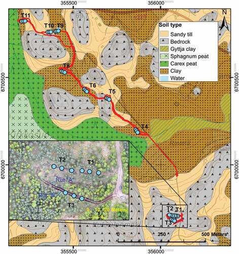
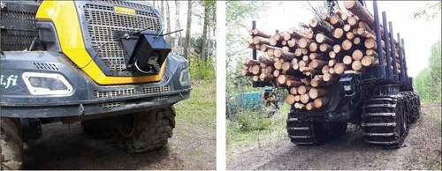
A field study was carried out in mid-May 2016 in Vihti, Southern Finland (X: 355,750 Y: 6,700,250 in ETRS-TM35FIN, 60°24.48ʹN, 24º23.23ʹE in WGS84). A route of 1.3 km (Figure 1) was driven first by an eight-wheeled Ponsse Scorpion King harvester with a mass of 22,500 kg. The rear wheels of each bogie were equipped with chains. Thereafter, a loaded eight-wheeled Ponsse Elk forwarder with a mass of 30,000 kg passed the route 2–4 times with varying driving directions. The rear wheels of the front bogie were equipped with chains and the rear bogie was equipped with Olofsfors Eco Tracks. Tire width was 710 mm in both the harvester and forwarder. The route passed through various soil types: clay, sandy till, and bedrock partly covered by 5–15 cm layer of fine-grained mineral soil and organic material (Figure 1). The terrain profile varied from flat to slightly undulating, and significant soil moisture variations occurred along the route. Part of the route was covered with logging residue.

Figure 1. Field test route (red line) and the ten 20-m-long test sites (light blue dots) located on various soil types. Test sites T1–T3 are enlarged into an aerial photo to show rut “A” and rut “B.” Source for soil map: GSF 1:20,000, for base map: NLS Topographic database 2016).

An outdoor version of a 2D Light Detection and Ranging (LiDAR) sensor (SICK LMS-511) was mounted in the back of the forest machines at a 45 degree angle (Figure 2). In the harvester, it was possible to mount the LiDAR sensor in the middle but in the forwarder, the sensor was mounted above the right-side back wheel. The first pass with the harvester and forwarder was driven in the same direction and every second forwarder pass was driven in the opposite direction ensuring equal scanning of both wheel ruts. The LiDAR sensor measured in 25 Hz frequency the distance and the angle to target ranging over 190 degrees with an angular resolution of 0.1667 degrees. Mounting the sensor at a 45 degree angle enabled the measurement of both the position and the speed independently from the forest machine’s Global Positioning System (GPS) through the identification of objects next to the ruts and above ground level as trees and calculating the distance traveled in relation to those tree objects. The speed measurements are not further dealt with in this article.

Figure 2. The 2D Light Detection and Ranging (LiDAR) sensor mounted on the rear of the Ponsse Scorpion King harvester (left) and on the Ponsse Elk forwarder (right).

For reference measurements, 10 ≈ 20-m long test sites were selected along the 1.3-km route (Figure 1). The rut depths were manually measured at 1-m intervals from both ruts (n ~ 40) after each vehicle pass (n = 3…5) using a horizontal hurdle and a measuring rod (Figure 3) to provide reference for the LiDAR-derived rut depths. Rut depths were measured from the lowest point in the perpendicular section of each measurement spot. Locations of manual measurement were marked on the ground with spray paint to enable consistent consecutive measurements between vehicle passes. Test site T2 was covered with logging residue to examine whether the LiDAR sensor was capable of detecting the ground surface through the brash mat. As this study was part of a larger research project, soil samples were also taken from each test site and analyzed in the laboratory for grain-size distribution, and organic matter fraction. However, only soil type is reported in this article.

Figure 3. Start and end points of the test sites were marked with a detectable structure made of boards (left). The depths of both ruts (“A” & “B”) were manually measured at 1-m intervals with a horizontal hurdle and measuring rod.

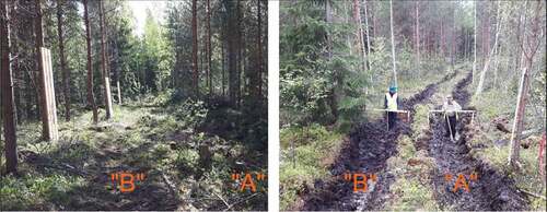
The ruts were labeled as rut “A” and rut “B” and their depth was measured after each pass in constant order despite the changing driving direction. Accurate GPS coordinates of the start and end points of the test sites were recorded, and marked with a structure made of three vertical pieces of board detectable in the point cloud produced by the LiDAR sensor (Figure 3). These structures were attached to remaining trees and the locations of these trees caused the lengths of the test sites to slightly differ from the intended 20 m.

Pre-processing of LiDAR sensor data to produce raw rut depth data

The LiDAR-derived point cloud data were processed with specially designed software developed by Argone Ltd to produce raw rut depth data with x- and y-coordinates. The outputs with 25 Hz frequency (40 ms interval) calculated from 2D LiDAR data included momentary position, vehicle speed and the maximum rut depth for rut “A” and rut “B”. Position and speed were calculated by recognizing the trees on both sides of the track from the point cloud data (Figure 4). This was mainly for allowing the comparison of LiDAR data to manual measurements in the test sites, and such procedure would not be needed for operational rut depth data collection. Test site start and end points were marked manually by the user when detecting the structures in the software.

Figure 4. Point cloud analysis and rut detection. Preliminary terrain level (thin blue line) is adjusted according to the terrain level found between the wheels (thick red line). Ruts were located and tracked with the Monte Carlo localization method. Circles (from left to right) indicate the points located in rut “A” (in green triangles), the points located between the ruts (in red stars) and the points located in rut “B” (in yellow squares). Temporary tree map (vertical cylinders) enables tracking the distance traveled.

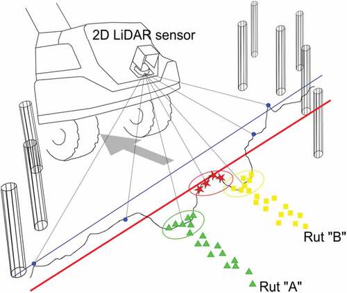
Wheel ruts were located and tracked by using a simple version of the Monte Carlo localization method (Thrun 2002), in which the position of the vehicle is used to forecast consecutive rut locations. The Monte Carlo filtering method limits the possible rut positions using the known tire width. Expected positions and related uncertainties of one standard deviation limited the measurement points that were used for rut depth estimation. The lowest point was selected from this subset of measurement points connected to each rut (green triangles within the green circle for rut “A” and yellow squares within the yellow circle for rut “B” in Figure 4) and this location was then used to forecast the filtered rut locations and uncertainties for the next measurement.

The point cloud data were divided into 1 m subparts perpendicular to the moving direction at each scan, i.e. every 40 ms, and the lowest point in each subpart was considered as representing the terrain level. The lowest 12.5% (1/8) and highest 37.5% (3/8) of these points were excluded and linear least squares method was used to fit a line to the remaining set of the points (thin blue line in Figure 4). This level of the terrain was then lowered or lifted according to the terrain level (thick red line in Figure 4) defined by the points located between the wheels (red star shapes circled in Figure 4) and this adjusted level was used as reference for calculating the rut depths.

Finally, rut depth was calculated simply as the difference between terrain level and the lowest point from the rut.

Data preparation and statistical analyses for comparison

Data for comparing LiDAR and manual rut depth measurements were picked from the raw rut depth data by taking an average of the raw rut depths located at ± 25 cm distance from the manual measurement spot.

The Kolmogorov-Smirnov test, Kruskal-Wallis test and Student’s t-tests (McDonald 2014) were performed for testing the similarity of the rut depth distributions from the manually measured and the LiDAR-derived rut depth data. Then, descriptive statistics were computed for manual and LiDAR measurements at each test site. The statistics included arithmetic average, standard deviation, root mean square error (RMSE) (Equation 1(1) $RMSE=\sqrt{\begin{array}{l}\frac{1}{N}\underset{N\left(pertestsiteandnoofpasses\right)}{\overset{i=1}{{{\displaystyle \sum }}^{\text{}}}}\hfill \\ {\left(LiDARderivedru{t}_i-manuallymeasuredru{t}_i\right)}^2\hfill \end{array}}$(1) ) firstly within the test site after each vehicle pass and secondly across all the test sites and machine passes. In addition to differences in test site means after each pass (Equation 2(2) $dif=\frac{1}{N}\sum _{i=1}^{N\left(pertestsiteofeachpass\right)}LiDARderivedru{t}_i\text{-}\frac{1}{N}\sum _{i=1}^{N\left(pertestsiteofeachpass\right)}manuallymeasuredru{t}_i$(2) ), the absolute differences were explored as percentages of the manually measured average (Equation 3(3) $difas\mathrm{\%}ofmanualaverage=\frac{\left|dif\right|}{manualmeanrut}\times 100$(3) ) and as a percentage of the standard deviation of manually measured ruts (Equation 4(4) $\begin{array}{l}difas\%ofmanualstd=\\ \frac{\left|dif\right|}{\sqrt{\begin{array}{l}\frac{1}{N-1}{\displaystyle {\sum }_{i=1}^{N\left(pertestsiteandnoofpasses\right)} }\\ {\left(manuallymeasuredru{t}_i-manualmeanrut\right)}^2\end{array}}}\times 100\end{array}$(4) ) to explore the differences in relation to magnitude of rut depths.

(1) $RMSE=\sqrt{\begin{array}{l}\frac{1}{N}\underset{N\left(pertestsiteandnoofpasses\right)}{\overset{i=1}{{{\displaystyle \sum }}^{\text{}}}}\hfill \\ {\left(LiDARderivedru{t}_i-manuallymeasuredru{t}_i\right)}^2\hfill \end{array}}$(1)

(2) $dif=\frac{1}{N}\sum _{i=1}^{N\left(pertestsiteofeachpass\right)}LiDARderivedru{t}_i\text{-}\frac{1}{N}\sum _{i=1}^{N\left(pertestsiteofeachpass\right)}manuallymeasuredru{t}_i$(2)

(3) $difas\mathrm{\%}ofmanualaverage=\frac{\left|dif\right|}{manualmeanrut}\times 100$(3)

(4) $\begin{array}{l}difas\%ofmanualstd=\\ \frac{\left|dif\right|}{\sqrt{\begin{array}{l}\frac{1}{N-1}{\displaystyle {\sum }_{i=1}^{N\left(pertestsiteandnoofpasses\right)} }\\ {\left(manuallymeasuredru{t}_i-manualmeanrut\right)}^2\end{array}}}\times 100\end{array}$(4)

A linear model and a linear mixed effects model were fitted to the calculated averages of the test sites per vehicle pass (n = 42 with 3–5 passes in the 10 test sites). If the LiDAR sensor measures the ruts similarly to the manual measurements, the regression slope should have a coefficient close to 1 and the intercept should be 0. We considered the effect of the test sites (e.g. varying soil type, Figure 1) by taking the test site as a random effect to the linear mixed effect model to explore potential site-specific errors that could affect the application of LiDAR-based method in varying sites.

All data processing was conducted in the R software (R Core Team 2017).

Results

Distributions of raw rut depth data

Variability of terrain and stand conditions on the test sites lead to highly varying rut depths. At some sites there were almost no ruts even after five vehicle passes, while almost 30-cm deep ruts were observed already after the first pass on sites most prone to rutting.

The two-sample Kolmogorov-Smirnov test conducted for the manually measured and LiDAR-derived rut depth data gave D = 0.13915 with a p-value of 1.7 × 10⁻¹⁴ indicating that the null hypothesis of same continuous distribution has to be rejected. Figure 5 shows the histograms of the raw ruts depths from both measurement techniques and the quantile-quantile (Q-Q) plots indicating the log-normally distributed manually measured rut depths (n = 1700) and exponentially distributed LiDAR-derived rut depths (n = 1659).

Figure 5. Histograms of manually measured raw rut depths (n = 1700) and LiDAR-derived rut depths (n = 1659) (left). Manually measured rut depths (middle) are log-normally distributed while the Light Detection and Ranging (LiDAR)-derived ruts depths (right) follow the exponential distribution.

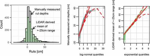
Based on the Kruskal-Wallis test and the Student’s t-test, however, the medians and means of the two rut depth datasets did not differ statistically (p-values for Kruskal-Wallis: 0.4954 and Student’s t-test: 0.2162).

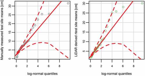
For the test site means of manual and LiDAR-derived datasets the Kolmogorov-Smirnov test gave D = 0.14286 with a p-value of 0.7848, and thus, according to null hypothesis the means calculated for the test sites with both measurement techniques followed the same log-normal distribution (Figure 6).

Figure 6. Log-normal Q-Q plot for manually measured test site means (left) and Light Detection and Ranging (LiDAR)-derived test site means (right). All vehicle passes are considered (n = 42).

Test site averages and descriptive statistics

The descriptive statistics together with the soil information from soil map (GSF 2015) and soil samples taken during the field campaign are shown in Table 1. While the overall RMSE for the mean rut depths across the test sites and vehicle passes was 3.5 (cm), in certain test sites (T2, T3, T10) the errors were higher than in others. Considering the ruts in rough classes of 0–10, 10–20 and deeper than 20 cm, we got five cases out of 42 where the LiDAR-derived ruts would fall in different classes compared to manually measured ruts (highlighted with light red and light blue in Table 1).

Table 1. Descriptive statistics of manually measured and LiDAR-based rut depths at each test site and test site soil characteristics. When classifying ruts to classes of < 10 cm, 10–20 cm and > 20 cm, the differing classification by LiDAR-derived ruts are marked with bold font (wavy underlined when underestimated rut class; double underlined when overestimated rut class).

Test site, soil type	Descriptive statistics	Manual					LiDAR
		1st pass	2nd pass	3rd pass	4th pass	5th pass	1st pass	2nd pass	3rd pass	4th pass	5th pass
T1	mean	3.7	5.2	6.4	6.7	6.9	4.1	5.3	5.5	6.8	6.2
bedrock fine sand moraine	std	4.5	4.5	4.7	4.0	4.4	4.7	6.6	6.7	5.9	6.7
	n	38	38	38	38	38	38	38	38	38	38
	RMSE						6.2	8.4	7.6	6.7	6.7
	dif in means						0.4	0.1	−0.9	0.1	–0.7
	dif as % of manual mean						10%	3%	15%	1%	10%
	dif as % of manual std						8%	3%	20%	3%	16%
T2	mean	1.9	2.1	4.1	4.8	4.6	4.7	8.8	7.0	8.3	7.7
(logging residue): bedrock/ coarse sand moraine fine sand moraine	std	4.5	6.4	5.5	5.4	5.8	10.8	8.6	9.4	9.3	8.1
	n	38	40	40	40	40	38	40	40	40	40
	RMSE						11.4	13.5	10.3	12.8	9.6
	dif in means						2.8	6.7	2.9	3.6	3.1
	dif as % of manual mean						149%	319%	70%	74%	67%
	dif as % of manual std						63%	105%	53%	66%	53%
T3	mean	7.9	11.6	17.8	25.2	30.1	4.9	4.0	16.5	17.8	25.5
bedrock/ clayish coarse sand clayish fine sand	std	6.4	7.8	12.6	14.9	15.6	8.8	10.3 40	16.9	16.2 40	20.4
	n	40	40	40	40	40	40		40		40
	RMSE						10.1	16.1	22.4	26.2	14.8
	dif in means						−3.0	−7.6	−1.2	−7.3	−4.5
	dif as % of manual mean						38%	66%	7%	29%	15%
	dif as % of manual std						46%	97%	10%	49%	29%
T4	mean	3.0	6.6	7.1	8.3	8.4	5.0	5.9	5.8	7.2	8.7
silty clay/clay	std	2.1	2.7	2.7	2.9	2.7	6.5	7.5	7.5	7.4	7.7
	n	42	42	42	42	40	42	42	42	42	40
	RMSE						6.5	7.3	7.1	7.4	6.8
	dif in means						2.0	−0.7	−1.3	−1.1	0.3
	dif as % of manual mean						67%	11%	18%	14%	4%
	dif as % of manual std						95%	26%	46%	39%	11%
T5	mean	2.2	4.2	4.9	5.6	5.7	2.5	6.2	4.2	7.5	4.0
bedrock/san d moraine/fine sand moraine	std	3.9	3.8	4.2	4.9	5.4	11.5	6.0	9.6	7.5	9.0
	n	32	40	40	40	40	32	40	40	40	40
	RMSE						12.4	8.1	11.1	9.2	10.9
	dif in means						0.3	2.1	−0.7	1.9	−1.7
	dif as % of manual mean						12%	50%	14%	33%	29%
	dif as % of manual std						7%	55%	16%	38%	31%
T6	mean	3.6	9.8	15.7	28.1	NA	1.2	7.5	10.4	25.4	NA
clay/ sandy silt	std	4.5	5.0	9.9	18.4		9.3	11.8	10.3	19.1
	n	40	40	38	36		40	40	38	36
	RMSE						11.8	12.5	13.1	23.0
	dif in means						−2.4	−2.3	−5.3	−2.7
	dif as % of manual mean						66%	23%	34%	10%
	dif as % of manual std						53%	45%	54%	15%
T8	mean	2.7	3.8	5.0	5.3	NA	10.0	3.9	3.7	6.9	NA
clayish fine	std	2.5	2.9	2.6	2.9		16.9	6.4	5.9	7.4
silt /clay	n	42	42	40	42		42	42	40	42
	RMSE						18.7	7.6	6.2	7.7
	dif in means						7.3	0.1	−1.5	1.6
	dif as % of manual mean						269%	3%	30%	30%
	dif as % of manual std						290%	3%	58%	56%
T9	mean	10.8	21.3	25.8	NA	NA	9.6	22.3	31.6	NA	NA
clay/ clayish coarse silt	std	7.4	10.3	13.7			12.1	13.1	18.6
	n	35	42	42			35	42	42
	RMSE						12.7	14.5	19.9
	dif in means						−1.2	1.0	5.8
	dif as % of manual mean						11%	5%	22%
	dif as % of manual std						16%	10%	42%
T10	mean	5.5	8.5	11.0	NA	NA	9.6	14.9	19.1	NA	NA
sand moraine/ fine sand	std	5.7	6.6	8.9			14.6 34	18.8 40	14.2
	n	34	40	40					40
	RMSE						17.7	20.5	15.7
	dif in means						4.1	6.5	8.1
	dif as % of manual mean						75%	76%	74%
	dif as % of manual std						72%	98%	91%
T11	mean	2.6	3.4	4.3	NA	NA	0.9	3.7	3.9	NA	NA
clay/ clayish medium silt	std	2.3	2.7	2.8			3.1	4.8	4.8
	n	32	36	42			32	36	42
	RMSE						4.6	5.8	4.5
	dif in means						−1.7	0.3	−0.4
	dif as % of manual mean						65%	10%	8%
	dif as % of manual std						73%	13%	13%
							RMSE per test site averages: 3.5

LiDAR, Light Detection and Ranging; RMSE, root mean square error

Testing performance with linear models and exploring sources of errors

The performance of the LiDAR sensor was further examined by fitting a linear model on the LiDAR-derived rut depth data to explain the manually measured average rut depths per test site after each vehicle pass. The linear model showed that the slope was close to 1 with a statistically significant p-value, while the intercept 0.32 was not significantly different from zero (Table 2). The standard error of residuals was 3.54 (cm). Figure 7 shows the manual rut depths plotted against the LiDAR-derived rut depths with the linear model depicted red line. The distribution of the points across the linear model (i.e. residuals) shows that there was no systematical over- or underestimation by the LiDAR sensor, and residuals were independent of magnitude of rut depth.

Table 2. Summary of linear model (Figure 7.) and linear mixed effect model statistics. T1…T11 are the test sites.

	Estimate	Standard error	t-value	p-value	Additional info:
linear model: manual test site means ~LiDAR-derived test site means	(intercept): 0.32	(intercept): 0.89	(intercept): 0.36	(intercept): 0.72	adj. R2: 0.77
n = 42	LiDAR: 0.93	LiDAR: 0.08	LiDAR: 11.80	LiDAR: 1.32e-14	res standard error: 3.54
mixed effect model: manual test site means ~LiDAR-derived test site means, random	(intercept): 0.83	(intercept): 1.16	(intercept): 0.72	(intercept): 0.48	within group res:
~1 test site	LiDAR: 0.86	LiDAR:	LiDAR:	LiDAR:	med: 0.15
n = 42	T1 intercept: 0.98 T2 intercept: −2.49	0.06	14.52	0.0000	Random effects:
groups:10	T3 intercept: 6.28				StdDev:
	T4 intercept: 1.07				(Intercept): 3.06 Residual: 1.98
	T5 intercept: 0.37
	T6 intercept: 4.39
	T8 intercept: −0.88
	T9 intercept: 1.11
	T10 intercept: −3.53
	T11 intercept: 0.98

LiDAR, Light Detection and Ranging.

Figure 7. Manually measured rut depth [cm] versus Light Detection and Ranging (LiDAR)-derived rut depth and the linear model fitted to the data (gray line).

The linear mixed effect model indicated that the intercept, while varying across the test sites (Table 2), was not statistically different from zero meaning that test site characteristics did not explain the variation better than the linear model. The slope was 0.86 which is further away from 1, and thus a poorer result compared to the slope of the linear model. The test sites with clearly different from zero values for the intercept (Table 2) were the ones where the errors were also the greatest. These test sites represented various conditions and the values were both under- and overestimated showing no pattern in measurement accuracy due to test site characteristics. The residuals of both models were normally distributed.

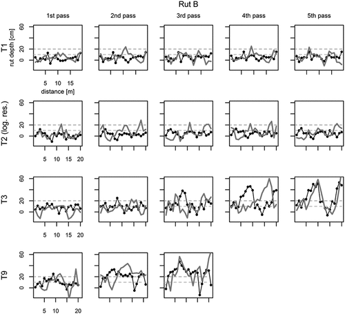
The manually measured and LiDAR-derived rut depths in four test sites are shown point-by-point in Figures 8 and 9. They suggest that in some test sites the LiDAR-derived and manually measured rut depths agreed well (in test site T1 for rut “A” and “B” and in test site T9 rut “A” 3rd pass). In other test sites there were possibly slight locational errors (rut “B” in test site T3 5th pass, rut “A” in test site T9 2nd pass) or clear mismatches (rut “A” in test site T3 3rd pass, for example) stemming from calculation errors. These errors, as will be discussed next, can be caused by poorly defined reference terrain level, errors in location calculation or in measured ruts or missed measurements due to tilting of the forest machine, for example.

Figure 8. Manually measured rut depths (black dotted line) and Light Detection and Ranging (LiDAR)-derived rut depths (thick gray line) on rut “A” in test sites T1, T2, T3, and T9. Test site T2 was covered with logging residue. The horizontal axis shows distance from beginning of the test site.

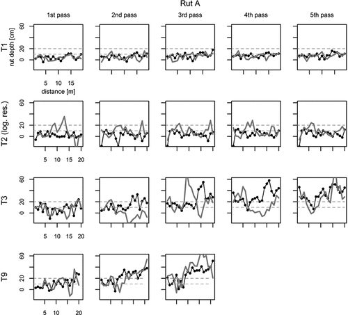
Figure 9. As Figure 8 but for rut “B.”

Discussion

Accuracy of LiDAR-based method and its potential for large-scale rut depth data collection

Based on our results from a single field study, we suggest that a forest machine-mounted LiDAR sensor can, with careful treatment of raw point cloud data, provide an efficient and reliable method for collecting rut depth data at 10–20 m spatial resolution. This resolution would be relevant for developing nationwide forest trafficability maps in Finland. The RMSE in test site averages was less than 3.5 cm for LiDAR compared to manual measurements, which was slightly higher than that of Pierzchała et al. (2016) for the photogrammetric method. Compared to their study, we did not adjust the data with the Iterative Closest Point (ICP) algorithm (that finds the smallest RMSE by rigid transformation to the dataset to be compared). In addition, our measurements were conducted during the harvest operation by a forest machine-mounted device when the measurement conditions are likely to be more challenging compared to post-operation conditions with measurements by a static device. Haas et al. (2016) also achieved more accurate rut depth measurements; however, their measurement setting was static and allowed before-after type comparison, which often leads to less error.

Hyyti and Visala (2013) report a study where two rotated 2D laser scanners were used to measure tree trunks and terrain from a moving all-terrain vehicle. They found the vehicle movement caused outliers to the data, and concluded the “mean” elevation of the 1 m grid terrain model was more robustly predicted by median than arithmetic average terrain level. In our study, no distinct difference between arithmetic average and median rut depths was found.

The test sites were about 20 m long and they varied in their soil and vegetation characteristics and surface topography; yet the LiDAR method provided rather accurate rut depth measurements across all test sites. This was confirmed by the linear model and particularly by the linear mixed effects model that showed no statistical significance for the intercept varying across the test sites (Table 2). These results suggest that the method is applicable across a range of forest conditions, a prerequisite for extensive data collection. While there are differences and clear dislocations, the manual measurements and the LiDAR-derived rut depths agree reasonably well, and that it was possible to distinguish test sites where deep ruts were formed and also those test sites where soil rutting was not occurring (Figures 8 and 9, Table 1). The increase in the rut depths after each pass was also well captured on the test sites where it took place (sites T3, T6, and T9).

The Government Decree on Sustainable Management and Use of Forests (1308/2013) based on the Finnish Forest Act (1093/1996) and related field control instructions by the Finnish Forest Centre (2013) regulate that ruts over 10 cm (mineral soils) and 20 cm (peatlands) are classified as damaged. The results show that the majority of rut depths measured by both methods were below 10 cm (Figures 5 and 7) and generally the errors did not depend on the magnitude of the rut depth. However, we had some test sites where rut depths were under- or overestimated with the LiDAR sensor and those are critical for ensuring reliable rut depth measurements. If we examine the ruts in rough classes of 0–10 cm, 10–20 cm and above 20 cm, five out of 42 cases (or 11.9%) were misclassified (i.e. under- or overestimated) by the LiDAR sensor measurements (Table 1). Considering the uncertainties related to manual measurements, this accuracy seems sufficient enough for collecting large-scale rut depth data at a 10–20 m resolution.

Challenges for rut depth measurements

Based on our results from LiDAR and manual measurements, it seems that difficulties in measuring the rut depth do not relate to the instrument per se but to the difficulty in defining the reference terrain level. In an undulating forest environment this is a difficult task both computationally and conceptually, and concerns both the LiDAR and manual measurements. Due to surface microtopography, dense understory vegetation and logging residue, the calculation of local terrain level is prone to random uncertainties that are reflected in the rut depth data. For instance, rocks and stumps between the wheels cause outlier values in the LiDAR-measured rut depth data. Due to these, rut depths can be overestimated at certain locations. On the other hand, a slight side slope downhill next to the trail can cause a rut depth that could be depicted as negative i.e. a “rut” to be above the reference terrain level. This might be a real case if the wheel dislocates a large amount of soil; however, in our test this occurred also at sites where soil was not displaced and accumulated. Despite the logging residue in test site T2 making the reference terrain level definition and rut depth measuring very challenging, our results showed that the LiDAR-based rut depths still agreed with manual measurements.

In operational applications we can overlook the need to match the LiDAR-derived rut depths to the exact location of manual measurements. However, we still need to consider the limitations to accurate measures stemming from the positioning inaccuracy if the data is being used for trafficability model development. The Global Navigation Satellite System (GNSS) improves the accuracy of the location information but still in some areas at certain times we might have up to a 10 m error in location (Kaartinen et al. 2015). This aspect influences the spatial resolution of the rut depth data, and thus the practical operational resolution would possibly lie somewhere between 10 and 20 m. We obtained our results for the 20 m section, but in some areas a shorter length could be more suitable if we consider that the standard deviation should not be equal to or higher than the mean (as opposite to some test sites in Table 1).

Implications of mounting the LiDAR sensor at a 45 degree angle

Several issues arise from the angle in which the LiDAR sensor is mounted on the forest machine. Firstly, underestimation of the rut depth can be brought by water gathering at the bottom of the rut between the few seconds of passing the point and measuring it due to the angle of the LiDAR sensor. On the wettest sites this is long enough for the water to cover the bottom of the rut. This effect can be minimized by direct downward mounting of the LiDAR sensor since the measurement occurs directly after the wheel has moved from the spot. Secondly, the terrain slope is not considered in the rut depth calculations and this naturally affects the LiDAR measurements as the angle varies along with the tilting of the forest machine. This could be corrected by a separate tilting sensor in the back of the forest machine. Tilting and rocking of the forest machine can cause the LiDAR beam to miss certain areas extending up to 50 cm in length despite the 25 Hz measurement frequency. Again, mounting the sensor facing directly downward would reduce the effect of tilting and rocking to the rut depth measurements and enable the sensor to reach more accurate rut depth results.

However, mounting the sensor directly downward reduces the ability to collect data on speed and location that was used in this study to facilitate point-by-point comparison of manually measured rut depths to the nearest LiDAR-based estimates. In addition, two LiDAR sensors would be required since scanning both ruts is not possible due to limited visibility when scanning directly downward. In mounting the LiDAR sensor at a 45 degree angle, one device is enough as our results (Figures 8 and 9) suggest that the right-side location of the sensor on the forwarder was not clearly detectable when examining the errors in the LiDAR-derived rut depths (the sensor was on top of rut “A” during the 3rd and 5th pass and on top of rut “B” during the 2nd and 4th pass).

Conclusions

Spatially and temporally extensive data on rut depths is needed for post-harvest quality control and for developing trafficability models based on open big data within the forest environment.

Using a tailored field experiment in real harvesting conditions, we evaluated whether forest machine-mounted LiDAR can provide a robust method for measuring rut depths caused by forest operations. We found that at a spatial resolution of 10–20 m, the LiDAR method provided unbiased estimates of rut depths with uncertainty (RMSE) comparable to that of other available methods. The LiDAR method shows great potential for operationalization. As Talbot et al. (2017) also recommend, mounting the LiDAR sensor on an operational forest vehicle can provide a cost-efficient tool for extensive on-site rut depth data collection as part of normal forestry operations.

Acknowledgments

We would like to thank Kalle Einola from Ponsse Oyj and Antti Peltola from Creanex Oy for technical support in data collection and analysis and Mr Ari Ryynänen (LUKE) for assisting in setting up the field study and data collection. Collaboration with Mr Lari Melander and Prof. Risto Ritala from the Technical University of Tampere is also greatly acknowledged. Prof. Juha Heikkinen (LUKE) is acknowledged for the help in refining the statistical methods. The two anonymous reviewers are also thanked for comments and suggestions for improvements. Overall the research project was enabled by the Academy of Finland Grant 295337, FOTETRAF.

Disclosure statement

No potential conflict of interest was reported by the authors.

Additional information

Funding

This works was supported by the Academy of Finland under Grant [295337, FOTETRAF]. Field studies were carried out in collaboration with project “Enhancing efficiency and quality of forest operations by benefitting information related working conditions (Metsäoperaatioiden tehostaminen ja laadun parantaminen olosuhdetiedon hyödyntämisen avulla)” coordinated by Finnish Natural Resources Institute (Luke) and funded by Ministry of Agriculture and Forestry of Finland (Maa- ja Metsätalousministeriö).

References

- Ågren AM, Lidberg W, Ring E. 2015. Mapping temporal dynamics in a forest stream network—implications for riparian forest management. Forests. 6:2982–3001.
- Ågren AM, Lidberg W, Strömgren M, Ogilvie J, Arp PA. 2014. Evaluating digital terrain indices for soil wetness mapping–a Swedish case study. Hydrol Earth Syst Sci. 18:3623–3634.
- Ala-Ilomäki J, Högnäs T, Lamminen S, Sirén M. 2011. Equipping a conventional wheeled forwarder for peatland operations. Int J For Eng. 22:7–13.
- Arbonaut Ltd./MEOLO. 2017. Staattinen kulkukelpoisuusluokitus [Static trafficability classification]. [accessed 2017 Sep 1]. Project website: https://www.luke.fi/projektit/meolo/
- Campbell DMH, White B, Arp PA. 2013. Modeling and mapping soil resistance to penetration and rutting using LiDAR-derived digital elevation data. J Soil Water Conserv. 68:460–473.
- Duncker PS, Raulund-Rasmussen K, Gundersen P, Katzensteiner K, De Jong J, Ravn HP, Smith M, Eckmüllner O, Spiecker H. 2012. How forest management affects ecosystem services, including timber production and economic return: synergies and trade-offs. Ecol Soc. 17:50.
- Finnish Forest Centre. 2013. Suomen metsäkeskuksen maastotarkastusohje [Field control instructions of Finnish Forest Centre]. [accessed 2016 Aug 1]. http://www.metsakeskus.fi/sites/default/files/smk-maastotarkastuohje.2013.pdf. Finnish.
- Forest Act of 1996. Ministry of agriculture and forestry of Finland. Forest Act (1093/1996). [accessed 2017 Aug 1]. http://www.finlex.fi/fi/laki/smur/1996/19961093.
- Forest Stewardship Council (FSC). 2015. FSC® international standard, FSC principles and criteria for forest Stewardship. [accessed 2017 Aug 1]. https://www.fsc.org/
- Geological Survey of Finland (GSF). 2015. Bedrock 1:200 000 and superficial deposits 1:20 000 and 1:50 000. [ accessed Apr 1] https://hakku.gtk.fi/en
- Goutal N, Keller T, Défossez P, Ranger J. 2013. Soil compaction due to heavy forest traffic: measurements and simulations using an analytical soil compaction model. Ann For Sci. 70:545–556.
- Haas J, Ellhöft KH, Schack-Kirchner H, Lang F. 2016. Using photogrammetry to assess rutting caused by a forwarder—a comparison of different tires and bogie tracks. Soil Tillage Res. 163:14–20.
- Hyyti H, Visala A. 2013. Feature based modeling and mapping of tree trunks and natural terrain using 3D laser scanner measurement system. IFAC Proc Vol. 46:248–255.
- Jaboyedoff M, Oppikofer T, Abellán A, Derron M, Loye A, Metzger R, Pedrazzini A. 2012. Use of LIDAR in landslide investigations: a review. Nat Hazards. 61:5–28.
- Jones M-F, Arp PA. 2017. Relating cone penetration and rutting resistance to variations in forest soil properties and daily moisture fluctuations. Open J Soil Sci. 7:149–171.
- Kaartinen H, Hyyppä J, Vastaranta M, Kukko A, Jaakkola A, Yu X, Pyörälä J, Liang X, Liu J, Wang Y, et al. 2015. Accuracy of kinematic positioning using global satellite navigation systems under forest canopies. Forests. 6:3218–3236.
- Kage T, Matsushima K. 2015. Rut detection using lasers and in-vehicle stereo camera. J Adv Control Autom Robot. 1:59–63.
- Klaes B, Struck J, Schneider R, Schüler G. 2016. Middle-term effects after timber harvesting with heavy machinery on a fine-textured forest soil. Eur J For Res. 135:1083–1095.
- Koreň M, Slančík M, Suchomel J, Dubina J. 2015. Use of terrestrial laser scanning to evaluate the spatial distribution of soil disturbance by skidding operations. iForest. 8:386–393.
- Labelle ER, Jaeger D. 2011. Soil compaction caused by cut-to length forest operations and possible short-term natural rehabilitation of soil density. Soil Sci Soc Am J. 75:2314–2329.
- Laurent J, Hébert JF, Lefebvre D, Savard Y 2012. Using 3D laser profiling sensors for the automated measurement of road surface conditions. In: 7th RILEM International Conference on Cracking in Pavements. 157–167. ( RILEM Bookseries, vol. 4)
- Liang X, Kankare V, Hyyppä J, Wang Y, Kukko A, Haggrén H, Yu X, Kaartinen H, Jaakkola A, Guan F, et al. 2016. Terrestrial laser scanning in forest inventories. J Photogramm Remote Sens. 115:63–77.
- Mäkisara K, Katila M, Peräsaari J, Tomppo E. 2016. The multi-source national forest inventory of Finland 2013. Helsinki: Natural Resources Institute Finland.
- McDonald JH. 2014. Handbook of biological statistics. 3rd ed. Baltimore, MD: Sparky House Publishing.
- McDonald TP, Stokes BJ, Aust WM. 1995. Soil physical property changes after skidder traffic with varying tire widths. J For Eng. 6:41–50.
- Murphy G, Brownlie R, Kimberley M, Beets P. 2009. Impacts of forest harvesting related soil disturbance on end-of-rotations wood quality and quantity in a New Zealand Radiata pine forest. Silva Fenn. 43:147–160.
- Murphy PNC, Ogilvie J, Arp P. 2009. Topographic modelling of soil moisture conditions: a comparison and verification of two models. Eur J Soil Sci. 60:94–109.
- Murphy PNC, Ogilvie J, Connor K, Arp PA. 2007. Mapping wetlands: A comparison of two different approaches for New Brunswick, Canada. Wetlands. 27:846–854.
- National Land Survey of Finland (NLS). 2017. The topographic database. [ accessed Apr 1] http://www.maanmittauslaitos.fi/en/e-services/open-data-file-download-service.
- Niemi M T, Vastaranta M, Vauhkonen J, Melkas T, Holopainen M. 2017. Airborne LIDAR-derived elevation data in terrain trafficability mapping. Scand J For Res. 32:762–773.
- Nugent C, Kanali C, Owende PM, Nieuwenhuis M, Ward S. 2003. Characteristic site disturbance due to harvesting and extraction machinery traffic on sensitive forest sites with peat soils. For Ecol Manag. 180:85–98.
- Ordonez C, Chuy OY, Collins EG, Liu X. 2011. Laser-based rut detection and following system for autonomous ground vehicles. J Field Robot. 28:158–179.
- Pierzchała M, Talbot B, Astrup R. 2014. Estimating soil displacement from timber extraction trails in steep terrain: application of an unmanned aircraft for 3D modelling. Forests. 5:1212–1223.
- Pierzchała M, Talbot B, Astrup R. 2016. Measuring wheel ruts with close-range photogrammetry. Forestry. 89:383–391.
- Programme for the Endorsement of Forest Certification (PEFC). 2010. International standard. PEFC Council, Luxembourg. [accessed 2017 Aug 1]. https://www.pefc.org/standards/technical-documentation/pefc-international-standards-2010
- R Core Team. 2017. R: A language and environment for statistical computing. Vienna (Austria): R Foundation for Statistical Computing.
- Saarilahti M. 2002. Soil Interaction model. University of Helsinki, Department of Forest Resources Management. [accessed 2016 Aug 1]. http://ethesis.helsinki.fi/julkaisut/maa/mvaro/publications/31/soilinte.pdf.
- Salmivaara A, Launiainen S, Tuominen S, Ala-Ilomäki J, Finér L. 2017. Topographic wetness index for Finland. Natural resources Institute Finland. Etsin research data finder.[accessed 2017 Aug 1]. http://urn.fi/urn:nbn:fi:csc-kata20170511114638598124
- Sirén M, Ala-Ilomäki J, Mäkinen H, Lamminen S, Mikkola T. 2013. Harvesting damage caused by thinning of norway spruce in unfrozen soil. Int J For Eng. 24:60–75.
- Smith CW, Johnston MA, Lorentz S. 1997. The effect of soil compaction and soil physical properties on the mechanical resistance of South African forestry soils. Geoderma. 78:93–111.
- Solgi A, Naghdi R, Labelle ER, Tsioras PA, Nikooy M. 2016. Effect of varying machine ground pressure and traffic frequency on the physical properties of clay loam soils located in mountainous forests. Int J For Eng. 27:161–168.
- Stenberg L, Tuukkanen T, Finér L, Marttila H, Piirainen S, Kløve B, Koivusalo H. 2016. Evaluation of erosion and surface roughness in peatland forest ditches using pin meter measurements and terrestrial laser scanning. Earth Surf Proc Landforms. 41:1299–1311.
- Suvinen A. 2006. A GIS-based simulation model for terrain tractability. J Terramech. 43:427–449.
- Suvinen A, Tokola T, Saarilahti M. 2009. Terrain trafficability prediction with GIS analysis. For Sci. 55:433–442.
- Talbot B, Pierzchała M, Astrup R. 2017. Applications of remote and proximal sensing for improved precision in forest operations. Croat J For Eng. 38:327–336.