Opportunity cost of several methods for determining forest biomass terminal locations in Northern Sweden

ABSTRACT

Long distance transportation of forest biomass is often unavoidable because the biomass is dispersed over large land areas. This is a problem that limits the development of biorefineries all over the world. The use of biomass terminals where forest biomass is transported to, stored, processed (mostly by mobile machinery), and reloaded can facilitate more environmentally friendly and efficient transportation to a biorefinery. The challenge is to identify the locations that should be selected for terminal establishment in order to minimize the cost of biomass procurement. In this study, locations for terminal establishment are proposed based on an optimization method (Combopt) that simultaneously minimizes the harvesting, transportation, and terminal costs for round wood and logging residues. The outcome of this method was compared with several other methods imitating situations with limited knowledge to estimate potential opportunity costs of potential knowledge deficiency when selecting terminal locations. The results of the Combopt method suggest that six terminals are required in order to minimize the overall cost of satisfying the estimated demand from the biorefineries. The opportunity cost of alternative terminal selection methods ranged from 3.1 to 35.4 million SEK (0.5–6.1% of total procurement cost). Methods that considered biomass relatively close to terminals had lower opportunity costs, together with methods minimizing transportation and terminal cost for the most common wood assortment. The methods and results could be applicable in other parts of the world were similar problems exists in forestry and other industries.

KEYWORDS:

• GIS
• logistics
• mixed integer programming
• transportation costs
• transport optimization
• satellite terminal

Introduction

To reduce the impact of human induced climate change, goals have been set to decrease the use of fossil fuel and feedstocks in the European Union and Sweden (European Commission 2011; Swedish Environmental Protection Agency 2012). This means that a shift to renewable sources is required with respect to both production processes and transportation. These changes rely on an adequate supply of renewable feedstock input, competitive production systems, and long term regulations allowing competition with fossil fuel products (Giuliano et al. 2016).

In Northern Sweden, there is currently a surplus of forest biomass (logs, small trees, logging residues, and stumps) (Fridh and Christiansen 2015; Athanassiadis and Nordfjell 2017). There are also several plans to build new biorefineries or expand existing ones in the area (e.g. Lundin 2017). However, the high costs of biomass procurement systems and lack of long term regulations have so far limited investments in the area (Börjesson et al. 2017). It is, therefore, important to reduce the cost of biomass procurement in order to support competitive alternatives to fossil fuel and feedstocks in Northern Sweden. Similar problems with high procurement costs potentially limiting development of biorefineries have also been noted in other parts of the world (e.g. Xie et al. 2014; Zhang et al. 2016; Broz et al. 2017; Araújo Júnior et al. 2017)

One way to reduce the cost and environmental impact of long-distance transportation of forest biomass is the use of terminals where biomass is reloaded to more environmentally friendly and efficient transportation options such as rail and high capacity trucks (Lindholm and Berg 2005; Tahvanainen and Anttila 2011; Jäppinen et al. 2014). Terminals for the handling and storage of goods have been used in Sweden for a long time. A location near the area that generates the goods and availability of suitable land for the establishment and geographic expansion of the terminal are considered important factors when building terminals (IBI Group 2006; Bergqvist et al. 2007). In addition, good connections to a high capacity and reliable railway system and proximity to major roads are important (IBI Group 2006). Important factors for the establishment of terminals specifically designed for forest biomass include the availability and price of forest biomass; opportunities for product refinement; a market for potential products and transportation facilities between the terminal and potential customers; expected profitability with respect to the market; sufficient expertise and experience in the organization (e.g. an experienced contractor hired for the day to day operation) and in operations management; fulfillment of requirements for safety, health and environmental legislation; and approval and support from local authorities (Dramm et al. 2002, 2004; Woody biomass 2010). These locations can be found through GIS methods that remove locations that do not fulfill the requirements (e.g. Zhang et al. 2011; Johnson et al. 2012), giving a number of potential terminals that can be evaluated further.

The challenge is to identify which terminals should be selected in order to minimize the costs of biomass procurement. There have been several analyses concerning the cost of forest biomass procurement and how to set up effective supply systems involving terminals (e.g. Rauch and Gronalt 2010; Kanzian et al. 2013; Virkkunen et al. 2016). It is relatively well-known that, from a theoretical point of view, mixed integer programming (MIP) that minimizes cost is the best approach to use when choosing between different terminal locations and transportation flows. However, in real situations, it is not always possible to use linear optimization to evaluate which terminals to build, because of the impact of other business decisions or a lack of information or knowledge about these methods. This means that often non-optimal approaches and methods are used to choose which terminal to use or build. This can incur an opportunity cost as the optimal choice might not be selected. It is, therefore, important to investigate how high this opportunity cost may be in order to allow a better trade-off in decisions about gathering information and obtaining knowledge in order to be able to use optimal methods for terminal location.

The aim of the study was to present a new model for locating biomass terminals optimally and optimizing the transportation flow in relation to the resource base, infrastructure, and industry location, and calculate the opportunity cost of using other methods for selecting terminal locations.

Materials and methods

Supply and demand

The supply of round wood (RW) and logging residues (LR) from one forest biomass supplier to meet the demands of three potential biorefineries located in Umeå (latitude 63.87,733, longitude 20.41,859), Örnsköldsvik (latitude 63.28,899, longitude 18.71,319) and Storuman (latitude 65.08615, longitude 17.11,342) in northern Sweden (Table 1) was investigated. Currently, in Umeå and Örnsköldsvik there are industrial facilities (pulpmills, sawmills, and district heating plants) that consume RW and LR, with plans for increased capacity, while the inland location of Storuman is a potential location for the establishment of a biorefinery at an old industry lot. All mass calculations were made on the basis of bone dry tonnes (BDt), see Table 2.

Table 1. Estimated raw material demand for potential biorefineries (in bone dry tonnes).

Source	Storuman	Umeå	Örnsköldsvik	Sum
Logging residues	50,000	120,000	180,000	350,000
Round wood	150,000	500,000	50,000	700,000

Table 2. Values used for conversion to bone dry tonne (BDt) in the study.

Source	Moisture content	BDkg/m^3solid ^C	kg/m^3solid ^C	BDkg/m^3loose ^C	kg/m^3loose^C	m^3top measured^C/ m^3solid^C
Logging residues	50^R	395^R	790^x	-	-	-
Logging residue chips	45^R	-	-	170^C	309^x	-
Roundwood	50^R	409^JC	819^x	-	-	1.56^C

- indicates no value. ^CChristiansen (2015). ^JC indicates that the value is estimated based on pine 408 BDkg/m³solid, spruce 382 BDkg/m³solid and that birch was assumed to be 20% heavier the spruce (458 BDkg/m³solid) (Jonsson 1985), and the proportion of tree species was 48% pine, 33% spruce, and 19% birch (Ringman 1996; Christiansen 2015). ^RRingman (1996). ^x indicates that the value was calculated based on density and moisture content.

The supply area considered was located in the inland part of northern Sweden, more specifically in the regions of Norrbotten, Västerbotten, and Jämtland, and consisted of the biggest forest owner category in terms of land area in the regions, namely all private forest owners and small institutional owners (FOCO).

Harvesting potentials for RW and LR from FOCO areas were extracted from the Skogliga konsekvensanalyser 2015 - SKA 15 (SKA 15) study (Claesson et al. 2015). SKA 15 includes estimates of forest development and forest fuel harvest potential obtained using the Heureka Regwise simulator (Wikstrom et al. 2011). The simulator used the sample plots (both permanent and temporary) of the Swedish forest inventory during the years 2008–2012 (Toet et al. 2007; Fridman et al. 2014; Fältinstruktion 2018). The estimates of the FOCO supply potential were based on sample plots located on FOCO estates. For sample plots, information on potential yearly harvest of RW (m³sub/year), and LR (BDt/year) was available. In total, 153 inventory plots appeared on the FOCO land, resulting in 153 assumed forest supply areas from which an annual biomass volume could be harvested sustainably.

These forest supply areas consisted of thinnings, regeneration felling (RF) and RF with seed trees (RFS). LR were considered for harvesting from RF and RFS with an uptake grade of 80% and 64% of the potential, respectively. These limits correspond to deliveries of LR from 90 of the forest supply areas. RW was assumed to be delivered from thinnings, RF and RFS, with an uptake grade of 100% of the potential. The total sustainable yearly harvestable potential was 779,289 and 399,261 BDt for RW and LR, respectively.

Potential terminals

Locations of potential terminals were identified as follows. First, a dot network with a distance of 10 km between the dots was applied over the region; in total, 217 dots were on FOCO land, and used in the subsequent analysis. Second, a buffer of 5 km was delimited adjacent to public BK1 roads (60 tonnes gross weight limit in trucks) (Swedish Transport Agency 2010) and railway lines, separately, using the Buffer tool in ARC-GIS 10.5 (Esri Inc., Redlands, California, United States). Forty-four dots were located within both buffers and considered as possible locations for building new terminals. Third, a distance matrix tool was created in ARC-GIS 10.5 in order to calculate the distances from each forest supply area to both the 44 potential terminals and the three biorefineries. The tool was also used to calculate the distances between potential terminals and the biorefineries. Different methods for selecting appropriate locations for establishing forest biomass terminals were then formulated, tested (Table 3), and evaluated based on total yearly overall cost in SEK i.e. the sum of overall terminal cost (TEC) in SEK and overall harvesting and transportation costs (PC) in SEK for RW and LR.

Table 3. Description of methods used to select terminals. The distance (D) from the forest to a terminal or between terminals used in stage 1, and the minimum permitted amount of biomass at a selected terminal (min T) is shown. Abbreviations: RW = round wood; LR = logging residues; TC = total cost; PC = overall harvest and transportation cost; TEC = overall terminal cost; MIP = mixed integer programming; LP = linear programming; SBR = Sturman biorefinery; and FSA = forest supply area.

					Explanation
Group	Method	Assortment in stage 1	D (km)	min T (BDt)	Stage one: selecting terminal to build	Stage two: Transportation	Stage 3: TC calculation
	Combopt	RW + LR	-	-	MIP, equation (1)*, for minimisation of TC, for both RW and LR simultaneously.	-	-
1	CtotRW	RW	-	-	MIP, equation (2)^+, for minimisation of PC and TEC for RW.	LP, equation (3)^x minimizing the PC for LR based on the terminals selected in stage 1	Equation (2) + (3)
	CtotLR	LR	-	-	MIP, equation (2)^+, for minimisation of PC and TEC for LR.	LP, equation (3)^x, minimizing the PC for RW based on the terminals selected in stage 1
2	CpcRW	RW	-	36,400	LP, equation (4)^Q, for minimisation of the PC for RW with at least min T at all selected terminals. Calculation of TEC based on the number of selected terminals.	LP, equation (3)^x, to minimize the PC for LR based on the terminals selected in stage 1, with no volume limitation	TEC was given by the number of terminals selected in stage 1. PC for RW by equation (4) and PC for LR by equation (3)
	CpcLR	LR	-	13,406	LP, equation (4)^Q, for minimisation of the PC for LR with at least min T at all selected terminals. Calculation of TEC was based on the number of selected terminals.	LP, equation (3)^x, minimizing the PC for RW based on the terminals selected in stage 1, with no volume limitation	TEC was given by the number of terminals selected in stage 1. PC for LR by equation (4) and PC for RW by equation (3)
3	DbT50	-	50	-	Based on D minimum distance from SBR. Step 1: All potential terminals within D distance of SBR were removed from the pool of potential terminals. Step 2: The nearest terminal in the pool) to SBR was selected, and all potential terminals within D distance of the selected terminal were removed from the pool of potential terminals. Step 3: This procedure was repeated until only selected terminals remained. TEC was calculated based on the number of selected terminals.	LP, equation (3)^x, to minimize the PC for RW and LR based on the selected terminals in stage 1. Deliveries in stage 2 were not bound to any of the constraints used in stage 1.	TEC was given by the number of terminals selected in stage 1. PC for both RW and LR was calculated in stage 2. PC for LR and RW by equation (3)
	DbT75	-	75	-
	DbT100	-	100	-
	DbT125	-	125	-
	DbT150	-	150	-
4	VT50RW	RW	50	36,400	Based on biomass availability within D distance of terminals. In this case SBR was treated as another terminal in step 1. Step 1: All FSA within D distance of a potential terminal were selected. When an FSA was within D distance or more from one potential terminal then all volume was assumed to be delivered to the nearest terminal. Step 2: If any potential terminal had deliveries below min T then the terminal with the smallest total delivery quantity was removed from the poll of potential terminals. Step 3: Steps 1 and 2 were repeated until all potential terminals in the pool had deliveries above min T. TEC is calculated based on the number of selected terminals.
	VT50LR	LR	50	13,406
	VT75RW	RW	75	36,400
	VT75LR	LR	75	13,406
	VT100RW	RW	100	36,400
	VT100LR	LR	100	13,406
5	VTS50RW	RW	50	36,400	Similar to Group 4, but SBR was treated with priority i.e. biomass from FSAs within D distance of SBR was delivered to SBR until the entire demand of SBR was met. First therafter could FSA within D Distances of SBR deliverer to any other terminal. The material closest to SBR was first delivered there before biomass from FSA further away was delivered there. Calculation of TEC was based on the number of selected terminals.
	VTS50LR	LR	50	13,406
	VTS75RW	RW	75	36,400
	VTS75LR	LR	75	13,406
	VTS100RW	RW	100	36,400
	VTS100LR	LR	100	13,406
6	VoltTRW	RW	-	36,400	Based on the assumption that the entire demand of all three biorefineries was delivered to terminals. Step 1: FSA were assigned to supply the investigated assortments to the closest potential terminal one by one based in distance beginning with the shortest distance, until the entire demand of the three biorefineries was satisfied. Step 2: If any terminal had deliveries below min T then the terminal with the smallest delivery quantity was removed from the pool of potential terminals. Step 3: Steps 1 and 2 were repeated until all terminals in the pool had deliveries above min T. These terminals were selected and TEC was calculated based on the number of selected terminals.
	VoltTLR	LR	-	13,406

*Equation (1) was subjected to constraints by Equations (5), (6), (7), (8), and (9). ⁺Equation (2) was constrained by equations (7), (10), (11), (12), and (13). ^xEquation (3) was constrained by Equations (14), (15), and (16). ^QEquation (4) was subjected to constraints by Equations (7), (12), (17), (18), (19), (20), and (21).

A reference method, Combopt, which minimized total yearly overall cost when selecting terminals to build in a one stage procedure considering PC for both assortments as well as TEC using MIP was formulated. An array of different methods that calculated total yearly overall cost in a three stage procedure (Table 3) was also formulated and tested. These methods either first selected terminals to build and minimized the PC for one assortment in stage 1 before minimizing the PC for the other assortment based on the selected terminal in stage 2, or first selected terminals to build in stage 1 and then minimized the transportation cost for both assortments based on the selected terminals in stage 2. In stage 3, total yearly overall cost was calculated based on the PC from stages 1 and 2, and TEC based on the number of selected terminals. The methods were clustered in six groups according to the methodology used to select terminals (Table 3). Several of the methods had limitations on the minimum permitted amount (BDt) of RW or LR at the terminals (Table 3). In the first stage, methods in Group 1 selected new terminal locations that minimized PC and TEC, by means of MIP, for one assortment, while methods in Group 2 selected new terminal locations that minimized PC, using LP, for one assortment with only a minimum volume requirement at selected terminals. In the methods that belong in the other groups, new terminal locations were selected depending on their distance to the potential biorefinery in Storuman as well as each other (Group 3), on biomass availability within a specified distance from a terminal, the potential biorefinery in Storuman and a minimum biomass requirement at selected terminals (Groups 4 and 5) or on the entire demand for biomass that was collected at terminals (Group 6). At the second stage, linear programming (LP) was used to minimize the PC of the second assortment for methods in Groups 1 and 2 and for both assortments for methods in Groups 3, 4, 5, and 6 (Table 3). Methods 3, 4, and 5 considered Storuman in the localization of terminals as Storuman is located in an area with many supply points and possible terminal points, while the other biorefineries are located further away from the possible terminals.

The MIP and LP were run in the Microsoft Excel based tool OpenSolver 2.9.0 using the COIN-OR CBC optimization engine (Mason 2012) (http://opensolver.org). Other calculations of terminal locations in Groups 3–6 were conducted in R (Core Team R 2015) using Rstudio Version 0.99.896 (R Studio Team 2015), and transportation flow was visualized in Rstudio with the ggmap library (Kahle and Wickham 2013).

Definitions of the constants and variables used in Equations (1)–(21) are given in Table 4.

(1) $MinTC=\sum _{i=1}^2\sum _{j=1}^{153}\sum _{k=1}^3\sum _{l=1}^{44}{V}_{ijkl}\ast CH{T}_{ijkl}+\sum _{i=1}^2\sum _{j=1}^{153}\sum _{k=1}^3{V}_{ijk}\ast CH{T}_{ijk}+\sum _{l=0}^{44}T{E}_l\ast CT$(1)

(2) $Min(P{C}_i+TEC)=\sum _{j=1}^{153}\sum _{k=1}^3\sum _{l=1}^{44}{V}_{jkl}\ast CH{T}_{jkl}+\sum _{j=1}^{153}\sum _{k=1}^3{V}_{jk}\ast CH{T}_{jk}+\sum _{l=0}^{44}T{E}_l\ast CT$(2)

(3) $MinP{C}_i=\sum _{j=1}^{153}\sum _{k=1}^3\sum _{l=1}^L{V}_{jkl}\ast CH{T}_{jkl}+\sum _{j=1}^{153}\sum _{k=1}^3{V}_{jk}\ast CH{T}_{jk}$(3)

(4) $MinP{C}_i=\sum _{j=1}^{153}\sum _{k=1}^3\sum _{l=1}^{44}{V}_{jkl}\ast CH{T}_{jkl}+\sum _{j=1}^{153}\sum _{k=1}^3{V}_{jk}\ast CH{T}_{jk}$(4)

(5) $FS{A}_{ij}\ge \sum _{k=1}^3\sum _{l=1}^{44}{V}_{ijkl}+\sum _{k=1}^3{V}_{ijk}\mathrm{\forall }ij$(5)

(6) $B{R}_{ik}\le \sum _{j=1}^{153}\sum _{l=1}^{44}{V}_{ijkl}+\sum _{j=1}^{153}{V}_{ijk}\mathrm{\forall }ik$(6)

(7) $TE\in \left\{0,1\right\}$(7)

(8) $T{E}_l\ast \sum _{i=1}^2\sum _{j=1}^{153}{V}_{ijl}=\sum _{i=1}^2\sum _{j=1}^{153}{V}_{ijl}\mathrm{\forall }l$(8)

(9) $V_{ijk},V_{ijkl},V_{ijl}\ge 0\mathrm{\forall }ijkl$(9)

(10) $FS{A}_j\ge \sum _{k=1}^3\sum _{l=1}^{44}{V}_{jkl}+\sum _{k=1}^3{V}_{jk}\mathrm{\forall }j$(10)

(11) $B{R}_k\le \sum _{j=1}^{153}\sum _{l=1}^{44}{V}_{jkl}+\sum _{j=1}^{153}{V}_{ijk}\mathrm{\forall }k$(11)

(12) $T{E}_l\ast \sum _{j=1}^{153}{V}_{jl}=\sum _{j=1}^{153}{V}_{jl}\mathrm{\forall }l$(12)

(13) $V_{jl},V_{jk},V_{jkl}\ge 0\mathrm{\forall }jkl$(13)

(14) $FS{A}_j\ge \sum _{k=1}^3\sum _{l=1}^L{V}_{jkl}+\sum _{k=1}^3{V}_{jk}\mathrm{\forall }j$(14)

(15) $B{R}_k\le \sum _{j=1}^{153}\sum _{l=1}^L{V}_{jkl}+\sum _{j=1}^{153}{V}_{jk}\mathrm{\forall }k$(15)

(16) $V_{jk},V_{jkl}\ge 0\mathrm{\forall }jkl$(16)

(17) $FS{A}_j\ge \sum _{k=1}^3\sum _{l=1}^{44}{V}_{jkl}+\sum _{k=1}^3{V}_{jk}\mathrm{\forall }j$(17)

(18) $B{R}_k\le \sum _{j=1}^{153}\sum _{l=1}^{44}{V}_{jkl}+\sum _{j=1}^{153}{V}_{jk}\mathrm{\forall }k$(18)

(19) $T{E}_l\ast minT\le \sum _{j=1}^{153}{V}_{jl}\mathrm{\forall }l$(19)

(20) $T{E}_l\ast \sum _{j=1}^{153}\sum _{l=1}^{44}{V_{jl}}_{jl}=\sum _{j=1}^{153}\sum _{l=1}^L{V}_{jl}\mathrm{\forall }l$(20)

(21) $V_{jl},V_{jk},V_{jkl}\ge 0\mathrm{\forall }jkl$(21)

Table 4. Parameters used in the optimization and/or calculation for Equations (1) - (21) and their abbreviation.

Variable	Definition	Comment
RW	Roundwood
LR	Logging residues
Vijkl	Amount (BDt) of assortment i transported from forest supply area j to biorefinery k through terminal l
Vijk	Amount (BDt) of assortment i transported from forest supply area j to biorefinery k
Vjkl	Amount (BDt) transported from forest supply area j to biorefinery k, through selected terminal l for investigated assortment (either RW or LR)
Vjk	Amount (BDt) transported from forest supply area j to biorefinery k for investigated assortment (either RW or LR)
Vijl	Amount (BDt) of assortment i transported to terminal l from forest supply area j
Vjl	Amount (BDt) transported from forest supply area j to terminal l for investigated assortment (either RW or LR)
CHTijkl	Cost (SEK/BDt) of harvesting and transporting assortment i from forest supply area j to biorefinery k through terminal l	CHTijl was added to the least expensive option for transportation between terminal l and biorefinery k.
CHTijk	Cost (SEK/BDt) of harvesting and transporting assortment i from forest supply area j to biorefinery k
CHTjkl	Cost (SEK/BDt) of harvesting and transportation from forest supply area j to biorefinery k, through selected terminal l for the investigated assortment (either RW or LR)	CHTjk was added to the least expensive option for transportation between terminal l and biorefinery k.
CHTjk	Cost (SEK/BDt) of harvesting and transporting from forest supply area j to biorefinery k for the investigated assortment (either RW or LR)
CHTijl	Cost (SEK/BDt) of harvest and transportation of assortment i from forest supply area j to terminal l
TEl	Decision variable to build terminal l
CT	Yearly operating and capital cost (SEK) of building one terminal
L	Selected terminals in stage 1 of the selection method
FSAij	The supply (BDt) of assortment i in forest supply area j
FSAi	The supply (BDt) in supply area j for the investigated assortment (either RW or LR)
BRik	Demand (BDt) of assortment i in biorefinery k
BRk	Demand (BDt) in biorefinery k for the investigated assortment (either RW or LR)
Min T	The minimum amount of the investigated assortment (either RW or LR) at a selected terminal.
TC	Total yearly overall cost (SEK/year)
PCi	Harvesting and transportation cost (SEK/year) for investigated assortment i
TEC	Total over all terminal cost (SEK/year)

The forest to terminal or biorefinery and terminal to biorefinery transportation cost was calculated based on fixed time and costs for different work elements, fixed machine costs and fees, and variable distance-dependent transportation costs. Tables 5 and 6 describe the input variables for calculating the cost of transporting from the forest to a terminal or biorefinery and from ta terminal to a biorefinery with trucks. From forest to terminal or biorefinery, LR had the transportation options of logging residue, chip, or chipper trucks. Logging residue trucks transport loose logging residues (has the sides and bottom of load space on the truck and trailer covered with metal plates), chip trucks transport chips (one chip bin on the truck and one on the trailer), and chipper trucks both comminute logging residue chips to chips and transport them (chipper and small chip bin on the truck and one chip bin on the trailer). RW could only be transported by round wood trucks. From terminal to biorefinery LR could be transported with chip trucks or by train and RW could be transported with round wood trucks or train.

Table 5. Input variables for calculating the cost for transportation of loose logging residues with logging residue trucks (LRT), transportation of logging residue chips with chip trucks or chipper trucks, and transportation of round wood with round wood trucks (RWT) from the forest to a terminal (T) or biorefinery (BR). Also shown are input variables for calculating the cost for transportation of round wood and logging residue chips between a terminal and biorefinery with chip trucks and train.

	From forest to terminal or biorefinery				From terminal to biorefinery
Variable	LRT	Chip truck T/BR	Chipper truck	RWT T/BR	Chip truck	RWT
Fixed machine costs
Investment (M SEK)	2.83^FB	2.5^BL	5.8^BL	2.9243^M	4^S	3.34^L
Service life (year)	5^FS	7^La	7^FS	7^FS	7^FS	7^La1
Interest (%)	5.5	5.5	5.5	5.5	5.5	5.5
Salvage value (SEK)	321,430^J	450,000^S	500,000^FS	157,248^M	600,000^S	179,601^M2
Tax (SEK/year)	40,000^FS	40,000^FS	25,000^NM	34,387^L	40,000^FS	41,402^L
Insurance (SEK/year)	65,000^FS	42,000^FS	70,114^NM	53,045^M	45,000^FS	55,450^L
Other fixed costs (SEK/year)	285,000^FS	39,500^FS	110,000^FS	137,000^L	40,000^FS	137,000^L1
Machine utilization
Workdays (No)	207^S	207^S	207^S	207^S	207^S	207
Shifts (No)	2	2	2	2	2	2
Hours (h/shift)	8.0	8.0	8.0	8.0	8.0	8.0
Utilization rate based on E15-h (%)^3	1.00	1.00	0.95	1.00	1.00	1.00
Operator costs
Personal cost (SEK/operator & year)	420,269	420,269	420,269	420,269	420,269	424,628
Variable machine cost
Fuel price ex. VAT (SEK/l)	12.5	12.5	12.5	12.5	12.5	12.5
Lubrication and hydraulic oil (SEK/l)	39	39	39	39	39	39
Fuel road, (l/10 km)	5.6^J	5.5^La	5.5^FS	5.73^L	4.97^A	5.6^JO
Fuel, loading (l/E15-h)	7.7^J	7^FS	48.7^EP	7^FS	7^FS	7
Fuel, unloading, (l/E15-h)	7.7^J	4^FS	4^FS	7^FS	4^FS	7
Lubrication and oil (l/E15-h)	0.05	0.05	0.05	0.05	0.05	0.05
Maintenance cost (SEK/10 km)	20^N	20^N	8.69^FS	17.2^JV	28.2^EH	27.6^EH4
Consumption material (SEK/BDt)	-	-	10	-	-
Other variable costs, (SEK/10 km)	5	4.61	5^FS	7.6^JV	-
Time consumption
Loading time (min)	47.5^N	77.6^BL	99^T	34^M	29.5^+	23.67^H4
Unloading time (min)	20^N	16.6^BL	20^N	17^M/3.67^H	16.6^Sam	4.69^H4
Waiting (min)	9.5^N	30/15	15	15	15	15
Velocity (km/h)	15–71^R	15–71^R	15–71^R	15–71^R	64^A	62^JV
Load size (BDt)	11.5^N
Load capacity (t)		37^La	28^JG	37.9^L	49.1^A	53.4^L
Load capacity (m^3)		129^La	100^T

-indicates no value. ^AAsmoarp et al. (2015). ^BLBerglund and Larsson (2012). ^EHEngström and von Hofsten (2015). ^EPEliasson and Picchi (2010). ^FBFriberg and Hansson (2012). ^HHamner (2014) ^JJoelsson et al. (2016). ^JGJohansson et al. (2014). ^JOJohansson (2015). ^JVJohansson and von Hofsten (2017). ^LLindström (2014). ^LaLaitila et al. (2016) (two shift). ^LJLaitila (2008). ^MMagnusson (2011) (including crane). ^NNäslund (2006). ^NMNilsson (2015). ^RRanta (2002) varies with transportation distance. ^SSpånberg (2016). ^TTrolin (2013). *indicates that the value is assumed to have the same relative difference as other trucks. ⁺indicates that the value is assumed increase or decrease relative to truck weight. ^Sam indicates that the value is assumed to be the same as for another truck. ^FSindicates that the value is assumed to increase or decrease relative to truck weight.¹ same as reported for 60 tonne truck. ²adjusted to 74 tonne based on the difference between investment cost in Magnusson (2011) and Lindström (2014). ³time, including delays shorter than 15 min. ⁴indicates that the value is assumed to increase relative to truck load in Lindström (2014).

Table 6. Fixed cost (SEK/BDt) for transportation of loose logging residues with logging residue trucks (LRT), transportation of logging residue chips with chip trucks or chipper trucks, and transportation of round wood with round wood trucks (RWT) from regeneration fellings (RF) and thinnings (TIN) to a terminal (T) or biorefinery (BR). Also shown are fixed costs for transporting round wood (RW) and logging residues chips (Chips) from a terminal to biorefinery with truck or train.

	From Forest					From Terminal
				Round wood truck		Truck		Train
Variable	LRT T/BR	Chipper truck T/BR	Chip truck T/BR	RF	TIN	Chips	RW	Chips	RW
Harvesting	-	-	-	130^BA	252^BA	-	-	-	-
Forwarding	209^A	209^A	209^A	98^A	157^A	-	-	-	-
Chipping	-	-	171^T	-	-	-	-	-	-
Loading	-	-	-	-	-	13^T1	7.34^S	13^T	7.34^S
Unloading	-	18^T/7^T	18^T/7^T	2.4^S	2.4^S	8^T1	4.3	8^T	4.3
Comminuting	121^T/96^T	-	-

-indicates no value. ^BBrunberg (2015). ^ABogghed (2013). ^BAindicates that the values were estimated from Bogghed (2013) and Brunberg (2006). ^BTindicates that the values were calculated based on Brunberg (2010) and Tahvanainen and Anttila (2011). ^SSondell (2006). ^TTahvanainen and Anttila (2011).¹ same as reported for trucks and trains.

Sixty tonne gross weight trucks were assumed to be used for transportation between the forest and a terminal or biorefinery, and 74 tonne gross weight trucks between a terminal and a biorefinery. These costs were calculated in the Excel application FLIS 4.0 Flexible lathund för interactive system analyse (Skogforsk 2011). The cost of train transportation of RW was based on Tahvanainen and Anttila’s (2011) cost per railway wagon or railroad car (wagon) and an assumed wagon load of 70 tonne (Engström and Winberg 2009). The calculation of the cost for LR was based on the function reported by Tahvanainen and Anttila (2011). The least expensive option for harvesting and transportation was always chosen. Based on these inputs, transportation costs were calculated. These functions were used to estimate procurement costs. The cost function for transportation from forest to terminal or to biorefinery included harvesting, forwarding, and unloading at the receiver. The cost function for transportation from terminal to biorefinery included loading and unloading costs.

Investment cost for a terminal was assumed to be 50,000,000 SEK, the depreciation period to be 20 years, and interest to be 7%. Other yearly cost of the terminal, regardless of biomass amount and assortments, was assumed to be 500,000 SEK. This resulted in a CT of 4,512,129 SEK/terminal.

Results

The opportunity cost of alternative methods of terminal selection ranged from 3.1 to 35.4 million SEK (Table 7). CtotRW had the lowest opportunity cost, followed by four methods (VTS50LR, VT50RW, VTS50RW, and VT50LR) that applied a minimum restriction on the amount of biomass that had to be delivered to selected terminals and also only considered forest supply areas that were situated 50 km or less from the terminals (Table 7). The methods in Group 3 that only considered distance between terminals had high opportunity costs (Table 7). The CpcLR method had the highest opportunity cost, while CpcRW was comparable to Group 3. In Group 4, methods that selected terminals based on LR availability at a specific distance from the terminal and limitation on the minimum permitted amount of LR at the terminals had a higher opportunity cost than methods based on RW (Table 7). The opposite was the case for Group 5 except that VTS100LR had a higher opportunity cost than VTS100RW. Methods in Groups 1 and 2 that used MIP for minimization of the TEC and PC for RW or LR, and in Group 6 had lower opportunity costs when RW was used in stage 1.

Table 7. The overall cost (kSEK) of harvesting and transporting round wood (RW) and logging residues (LR) from a forest supply area to biorefinery, overall costs for terminals (TEC), overall total cost (TC), and opportunity cost for non-optimal methods. “No” indicates number of selected terminals.

		PC (kSEK)		Terminal
	Method	RW	LR	No	TEC (kSEK)	TC (kSEK)	Opportunity cost (kSEK)
Group	Combopt	339,685	218,197	6	27,073	584,955	-
	CtotRW	346,412	223,565	4	18,049	588,025	3,071
	CtotLR	360,626	225,458	3	13,536	599,620	14,665
	CpcRW	330,766	211,572	13	58,658	600,997	16,042
	CpcLR	329,319	209,820	18	81,218	620,357	35,403
	DbT50km	333,525	213,608	16	72,194	619,327	34,373
	DbT75km	334,053	213,660	12	54,146	601,858	16,904
	DbT100km	339,643	217,394	10	45,121	602,158	17,204
	DbT125km	355,253	227,808	6	27,073	610,134	25,180
	DbT150km	361,629	231,045	4	18,049	610,723	25,768
	VT50RW+	339,320	216,930	8	36,097	592,347	7,392
	VT50LR	337,769	214,399	9	40,609	592,776	7,822
	VT75RW*	332,490	212,940	11	49,633	595,063	10,109
	VT75LR	333,030	211,148	12	54,146	598,324	13,370
	VT100RW*	332,490	212,940	11	49,633	595,063	10,109
	VT100LR	332,710	210,607	14	63,170	606,487	21,532
	VTS50RW+	339,320	216,930	8	36,097	592,347	7,392
	VTS50LR	337,978	215,719	8	36,097	589,794	4,840
	VTS75RW*	332,490	212,940	11	49,633	595,063	10,109
	VTS75LR	333,030	211,978	11	49,633	594,641	9,687
	VTS100RW*	332,490	212,940	11	49,633	595,063	10,109
	VTS100LR	332,710	211,134	12	54,146	597,990	13,035
	VoltTRW*	332,490	212,940	11	49,633	595,063	10,109
	VoltTLR	333,597	211,340	12	54,146	599,082	14,127

+indicates that the same terminals were selected in VT50RW and VTS50RW. * indicates that the same terminals were selected in VT75RW, VT100RW, VTS75RW, VTS100RW, and VoltTRW.

The Combopt method selected six terminals, compared to four and three terminals for the CtotRW and CtotLR methods, respectively (Table 7, Appendix A). In Group 3 the number of selected terminals decreased as the distance between terminals and between terminals and a biorefinery increased. The opposite was the case for methods in Groups 4 and 5 when biomass availability within certain distances from the terminal was considered (Appendix A, Table 7). Some methods with high opportunity costs selected terminals that, when it came to the LP in stage 2, were only used for one assortment or not used at all. This was the case for VT100LR and VTS75LR, where one selected terminal was not used for either RW nor LR in stage 2. VT75LR and VT100LR had one terminal and VoltTLR two terminals that were only used for LR transportation in stage 2 (Appendix A).

There were examples of forest supply areas delivering biomass both to a terminal and directly to a biorefinery in the Combopt method, but also in some of the other methods (Appendix A). There were also examples of forest supply areas delivering RW and LR directly to two biorefineries, e.g. CtotRW. Forest supply areas could also deliver to two different terminals; this occurred in the CtotLR, CtotRW, and DbT150km methods. In most of the methods that selected a small number of terminals, the majority of those delivered material to the biorefineries in Umeå and Örnsköldsvik, while it was more common that terminals only delivered to one biorefinery in methods that selected more terminals.

In all methods, the entire demand of Storuman for RW and LR was delivered directly to the biorefinery in stage 2 (Table 8). The other biorefineries had a varying amount of direct delivery depending on the method of terminal selection. In all methods, the biorefinery in Umeå had some direct delivery of RW. Direct deliveries of LR to Umeå and of RW and LR to Örnsköldsvik only occurred in some of the methods (Table 8).

Table 8. Amount of biomass (BDt) transported directly from forest supply area to biorefineries in Storuman (S.uman), Örnsköldsvik (Övik), and Umeå, and the amount first transported to terminal (Terminal) for reloading before transportation to biorefinery.

	Round wood						Logging residues
	Directly			Through terminal			Directly			Through terminal
Method	S.uman	Övik	Umeå	S.uman	Övik	Umeå	S.uman	Övik	Umeå	S.uman	Övik	Umeå
Combopt	150,000	0	45,132	0	50,000	454,868	50,000	0	15,646	0	180,000	104,354
CtotRW	150,000	19,649	49,867	0	30,351	450,133	50,000	6,365	21,694	0	173,635	98,306
CtotLR	150,000	50,000	52,298	0	0	447,702	50,000	21,704	15,646	0	158,296	104,354
CpcRW	150,000	12,410	5,945	0	37,590	494,055	50,000	0	0	0	180,000	120,000
CpcLR	150,000	0	12,221	0	50,000	487,779	50,000	0	0	0	180,000	120,000
DbT50km	150,000	0	23,751	0	50,000	476,249	50,000	0	0	0	180,000	120,000
DbT75km	150,000	0	12,221	0	50,000	487,779	50,000	0	0	0	180,000	120,000
DbT100km	150,000	0	12,221	0	50,000	487,779	50,000	0	0	0	180,000	120,000
DbT125km	150,000	42,430	45,132	0	7,570	454,868	50,000	19,687	15,646	0	160,313	104,354
DbT150km	150,000	46,574	52,298	0	3,426	447,702	50,000	19,687	21,694	0	160,313	98,306
VT50RW+	150,000	13,515	12,221	0	36,485	487,779	50,000	6,365	0	0	173,635	120,000
VT50LR	150,000	5,205	12,221	0	44,795	487,779	50,000	0	0	0	180,000	120,000
VT75RW*	150,000	0	12,221	0	50,000	487,779	50,000	0	0	0	180,000	120,000
VT75LR	150,000	0	12,221	0	50,000	487,779	50,000	0	0	0	180,000	120,000
VT100LR	150,000	0	12,221	0	50,000	487,779	50,000	0	0	0	180,000	120,000
VTS50LR	150,000	13,515	12,221	0	36,485	487,779	50,000	6,365	0	0	173,635	120,000
VTS75LR	150,000	0	12,221	0	50,000	487,779	50,000	0	0	0	180,000	120,000
VTS100LR	150,000	0	12,221	0	50,000	487,779	50,000	0	0	0	180,000	120,000
VoltTLR	150,000	0	12,221	0	50,000	487,779	50,000	0	0	0	180,000	120,000

+indicates that method VTS50RW also gave the same terminal locations. * indicates that methods VT100RW, VTS75RW, VTS100RW, and VoltTRW also gave the same terminal location.

Discussion

The Combopt method identified the most cost efficient solutions to the terminal location and transportation problem. This was mainly due to the fact that it considered interaction effects between RW and LR when selecting terminals---something that no other method did. The opportunity cost was larger than expected, especially for CtotLR (Table 7). This fact highlights the importance of considering as many assortments as possible when analyzing the terminal and transportation cost and solving optimization problems with MIP. The positive effect of considering more than one assortment has been noted previously (Xie et al. 2014; Abasian et al. 2017). These results indicate that it could be worth the time and money spent on gathering information and gaining knowledge to be able to use MIP methods to consider several assortments simultaneously.

However, in practice, it can be difficult to obtain the information required and a method involving opportunity costs might be applied. Sometimes, it can also occur that a conscious business decision is made to use a method that has opportunity costs because of other business or personal considerations (Bergqvist et al. 2010). In these situations, it is important to know which methods are the most suitable to use. From the results in our study, it appears that the methods that consider biomass availability within 50 km of the terminals have lower opportunity costs than other methods. It also seems important to include other industries in the analysis as the methods in Group 5 had lower opportunity costs than those in Group 4 for LR (Table 7, Appendix A). The reason for the difference was that the biorefinery in Storuman was treated differently in the two groups when selecting terminal locations; thus, no terminal could be selected close to the biorefinery when using a method from Group 5, while this could happen when using the Group 4 methods. When RW was investigated, there were no differences between equal distance methods in Groups 4 and 5, due to the distribution of biomass in the forest supply areas around Storuman and that the annual minimum volume for a terminal was higher for RW than LR. This difference in minimum annual volume led to the situation where almost all methods using volume limitations selected more terminals for LR than for RW (Table 7). The methods in Group 3 that used only distance between terminals as a criterion for terminal selection could be useful in a situation where the biomass is evenly distributed across the area. However, this is not a realistic assumption in most practical applications as the biomass potential is unevenly distributed due to previous management, site productivity, and other land uses and this variation was demonstrated by Lundmark et al. (2015) in Sweden for logging residues and pulpwood.

The methods in Groups 1 and 2, which in stage 1 selected terminals through MIP considering one assortment (Table 5), cannot generally be recommended. Although the opportunity cost for CtotRW was low, the opportunity cost for CtotLR was high. Neither the CpcRW nor the CpcLR methods can be recommended due to their high opportunity cost, unless there is a strong belief that the transportation cost to a terminal will become extremely important in the future. However, such a belief would be better addressed by increasing the transportation cost in a MIP model that, instead of a minimum required volume at a terminal, it includes terminal cost. Furthermore, in Group 2, forest supply areas delivered biomass to more than one terminal only to “unlock a terminal”; i.e. delivering a small volume in order to reach the minimum annual volume, so other forest supply areas could deliver to it. This situation leads to a higher transportation cost than necessary, and it is therefore better to use the terminal construction cost than a minimum volume when analyzing terminal location. This indicates that, if MIP for one assortment is used in stage 1, it should be for the most common assortment. Currently, it is also most common that forest fuel terminals host logging residue chips, loose logging residues, and bark despite the fact that they could accommodate up to 14 different biomass assortments (Kons et al. 2014).

All transportation to Storuman, regardless of method, was made directly to the biorefinery without passing through a terminal, as the plant was located in the middle of a cluster of forest supply areas with short distances to Storuman. These results were in line with previous findings, indicating that the transportation distance using trains had to be sufficient to cover the cost of transferring goods from truck to train (Mahmudi and Flynn 2006; Tahvanainen and Anttila 2011). Some of the RW deliveries to Umeå were also delivered directly from the forest to the biorefinery, regardless of method for the same reason. These results highlight the importance, in the analysis of terminal location, of including direct transportation to plants both near and further away from the biomass supply area. Similar results have been found in previous studies (e.g. Rauch and Gronalt 2010).

The VT100LR and VTS75LR methods selected terminals in stage 1 that were not used in stage 2, as it was less expensive to transport the material elsewhere even though the cost of terminal construction had already been accounted for. A similar situation was observed in other studies where the cost of unloading the truck and reloading to another means of transport was too high to make reloading viable (Mahmudi and Flynn 2006; Tahvanainen and Anttila 2011). This indicates that it is not always optimal to use an existing terminal as the cost of unloading and reloading may outweigh the reduction in transportation cost.

The method of first using GIS to determine possible terminal locations based on different criteria and then using other methods to evaluate the attractiveness of the locations seemed to work well in our study and has been used previously in forest logistics (e.g. Johnson et al. 2012). Similar methods can also be used to evaluate the location of industries and Zhang et al. (2011) demonstrated for a possible biorefinery in Northern Michigan by first finding suitable locations based on infrastructure and then comparing them based on transportation cost. Terminal or industry locations can also be evaluated using e.g. different gravity methods or an analytical hierarchy process (Zettergren and Bergsten 2010; Alam 2013). However most of these values could be included in a MIP model by adding different restrictions. We therefore think that LP or MIP is preferable.

There are several factors that were not considered in our study. First, there are at least four round wood assortments, hard- and softwood pulp, and pine and spruce saw timber. Secondly, there are several more biorefineries, sawmills, and heating plants in the area that affect the flow of biomass. Thirdly, there are also several other forest owners, although some of them supply to their own industry so their biomass may not be available to other plants. These factors could very well influence the total yearly overall cost of different methods. However, we do not believe that it would change which methods are preferable when the Combopt method cannot be used. These factors were therefore not included in the analysis in our study but could be interesting to include in future studies.

Similar problems to the one that we investigated in this study are present in the forest sector in other parts of the world, and in other sectors when considering different terminal locations (e.g. Sörensen et al. 2012; Xie et al. 2014; Zhang et al. 2016; Broz et al. 2017). The difference between the methods should be roughly thesame in other conditions i.e. which method is best to use. Thereshould be differences, however, in the relative or absolute magnitude of the various methods as this depends on the site conditions and industry characteristics.

In conclusion, the reference method that considered both assortments and terminal location in a mixed integer programming model was clearly the best choice. The difference between the reference method and the other methods was large enough to warrant acquiring knowledge and collecting information to allow the use of a mixed integer programming model for similar situations. If only one assortment is used in a MIP model, then the largest assortment should be the one examined. When using trivial methods, using the volume within about 50 km or less from the terminal seemed to be most advantageous, even though it was far worse than the reference model.

Disclosure statement

No potential conflict of interest was reported by the authors.

Additional information

Funding

The study was funded partly by the Interreg Botnia-Atlantica programme and partly by Österbottens förbund (FI), Region Västerbotten (SE), Naturresursinstitutet (FI), Länsstyrelsen Västernorrland (SE), Sveriges lantbruksuniversitet (SE), Terminalen i Bastuträsk (SE), Biofuel Region Brf AB (SE), Seinäjoki yrkeshögskola (FI) and Keski-Pohjanmaan koulutusyhtymä (FI).

Appendix A: Biomass flow

short-legendFigure A1.

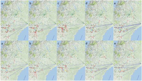
The biomass flow from forest to biorefinery for roundwood (top) and logging residues (bottom). Panel A Combopt method, panel B CtotRW method, panel C CtotLR method, panel D RWtrpcT method, and panel E, LRtrpcT method. Green dots represent forest supply areas, red dots represent selected terminals, orange dots represent potential terminals that were not selected, blue dots represent biorefineries, green lines represent biomass flow from forest supply areas to terminals, red lines represent biomass flow between forest supply areas and terminal, and blue lines represent biomass flow between terminals and biorefinery.

short-legendFigure A2.

The biomass flow from forest to biorefinery for roundwood (top) and logging residues (bottom). Panel A DbT50 km method, panel B DbT75 km method, panel C DbT125 km method, panel D VT50RW and VTS50RW methods, and panel E, VT75RW, VT100RW, VTS75RW, VTS100RW, and VoltTRW methods. Green dots represent forest supply areas, red dots represent selected terminals, orange dots represent potential terminals that were not selected, blue dots represent biorefineries, green lines represent biomass flow from forest supply areas to terminals, red lines represent biomass flow between forest supply areas and terminal, and blue lines represent biomass flow between terminals and biorefinery.

short-legendFigure A3.

The biomass flow from forest supply areas to biorefinery for roundwood (top) and logging residues (bottom). Panel A VT50LR method, panel B VT75LR method, panel C VT100LR method, panel D VTS75LR method, and panel E, VoltTLR method. Green dots represent forest supply areas, red dots represent selected terminals, orange dots represent potential terminals that were not selected, blue dots represent biorefineries, green lines represent biomass flow from forest supply areas to terminals, red lines represent biomass flow between forest supply areas and terminal, and blue lines represent biomass flow between terminals and biorefinery.

References

- Abasian F, Rönnqvist M, Ouhimmou M. 2017. Forest fibre network design with multiple assortments: a case study in Newfoundland. Can J For Res. 47(9):1232–1243.
- Alam SA. 2013. Evaluation of the potential locations for logistics hubs: a case study for a logistics company [master’s thesis]. Stockholm: Royal Institute of Technology, Department of transport science.
- Araújo Júnior CA, Leite HG, Soares CPB, Binoti DHB, de Souza AP, Santana AF, Torre CMME. 2017. A multi-agent system for forest transport activity planning. Cerne. 23(3):329–337.
- Asmoarp V, Jonsson R, Funck J. 2015. Fokusveckor 2015-Bränsleuppföljning för ett 74 tons flisfordon inom projektet ETT-Flis [Focus weeks 2015 - Fuel consumption follow -up for a 74 tonne chip truck within the project ETT-Flis]. Uppsala: Skogforsk. Arbetsrapport 890. Swedish.
- Athanassiadis D, Nordfjell T. 2017. Regional GIS-based evaluation of the potential and supply costs of forest biomass in Sweden. Front Agr Sci Eng. 4(4):493–501.
- Berglund M, Larsson J. 2012. En jämförande kostnadsanalys av maskinsystem för upparbetning och transport av GROT [A comparative cost analysis of machine systems for chipping and transport of logging residues]. Umeå: Swedish University of Agricultural Sciences, Department of Forest Resource Management. Arbetsrapport 366. Swedish.
- Bergqvist R, Falkemark G, Woxenius J. 2007. Etablering av kombiterminaler [Establishing intermodal terminals]. Göteborg: Chalmers University of Technology, Division of Logistics and Transportation. Meddelande 124. Swedish.
- Bergqvist R, Falkemark G, Woxenius J. 2010. Establishing intermodal terminals. World Rev Intermodal Transp Res. 3(3):285–302.
- Bogghed A. 2013. Skogsbrukets kostnader 2013 - Norra, mellersta och södra Sverige [Forestry costs 2013 – north, mid and south Sweden]. Gävle: Lantmäteriet. Rapport. 2013:4. Swedish.
- Börjesson P, Hansson J, Berndes G. 2017. Future demand for forest-based biomass for energy purposes in Sweden. For Ecol Manag. 383:17–26.
- Broz D, Durand G, Rossit D, Tohmé F, Frutos M. 2017. Strategic planning in a forest supply chain: a multigoal and multiproduct approach. Can J For Res. 47:297–307.
- Brunberg T. 2006. 2005’ – stormens år [2005 – the year of the storm]. Uppsala: Skogforsk. Resultat 11. Swedish.
- Brunberg T. 2010. Skogsbränsle: metoder, sortiment och kostnader 2009 [Forest fuel: methods, assortments and costs 2009]. Uppsala: Skogforsk. Resultat 12. Swedish.
- Brunberg T. 2015. Skogsbränsle - trender över 5 år [Forest fuel trends over 5 years]. In: Iwarson-Wide M, Palmer CH, editors. Skogensenergi -en källa till hållbar framtid [Forest energy for source to sustainable future]. Uppsala: Skogforsk; p. 36–37. Swedish.
- Christiansen L, editor. 2015. Skogsstatistisk årsbok 2014 [Swedish statistical yearbook of forestry]. Jönköping: Swedish Forest Agency. Swedish.
- Claesson S, Duvemo K, Lundström A, Wikberg P-E. 2015. Skogliga konsekvensanalyser 2015 – SKA 15 [Forest consequence analysis 2015 - SKA 15]. Jönköping: Swedish Forest Agency. Rapport 10. Swedish.
- Core Team R. 2015. R: A language and environment for statistical computing. Vienna (Austria): The R Foundation for Statistical Computing.
- Dramm J R, Govett R, Bilek T, Jackson GL. 2004. Log sort yard economics, planning, and feasibility. Madison (WI): U.S. Department of Agriculture, Forest Service, Forest Products Laboratory.
- Dramm JR, Jackson G, Wong J. 2002. Review of log sort yards. Madison (WI): U.S. Department of Agriculture, Forest Service, Forest Products Laboratory. Report FPL−GTR−146.
- Eliasson L, Picchi G. 2010. Huggbilar med lastväxlare och containrar [Cipper trucks with container system]. Uppsala: Skogforsk. Arbetsrapport 715: 2010. Swedish.
- Engström J, Winberg P. 2009. Systemtransporter av skogsbränsle på järnväg [System transports of forest fuels on train]. Uppsala: Skogforsk. Arbetsrapport 678:2009 Swedish.
- Enström J, von Hofsten H. 2015. ETT-Flis 74-ton - En projektrapport över drifttagande och ett års uppföljning av tre 74-tons flisfordon [ETT-Chips 74-tonne trucks - Three 74-tonne chip trucks monitored in operation over one year]. Uppsala: Skogforsk. Arbetsrapport 888:2015 Swedish.
- European Commission. 2011. A Roadmap for moving to a competitive low carbon economy in 2050. Brussels: Communication from the commission to the european parliament, the council, the european economic and social committee and the committee of the regions. COM(2011) 112 final.
- Fältinstruktion. 2018. Fältinstruktion 2018 RIS-Riksinventeringen av skog [Field instructions 2018 RIS- national inventory of forest]. Umeå: Swedish University of Agricultural Sciences, Department of Forest Resource Nanagement and Swedish University of Agricultural Sciences, Swedish Forest Soil Inventory. Swedish.
- Friberg G, Hansson J. 2012. Kostnadskalkyl för flis med terminalhantering på Basamyran [Cost calculation for wood chips with terminal handling at Basamyran]. Umeå: Swedish University of Agricultural Sciences, Department of Forest Resource Management. Arbetsrapport 372. Swedish.
- Fridh M, Christiansen L. 2015. Rundvirkes- och skogsbränslebalanser för år 2013 – SKA 15 [Roundwood and forest fuel balances for year 2013 - SKA 15]. Jönköping: Swedish forest agency. Meddelande 3. Swedish.
- Fridman J, Holm S, Nilsson M, Nilsson P, Ringvall AH, Ståhl G. 2014. Adapting national forest inventories to changing requirements – the case of the Swedish national forest inventory at the turn of the 20th century. Silva Fenn. 48(3): 1-29.
- Giuliano A, Poletto M, Barletta D. 2016. Process optimization of a multi-product biorefinery: the effect of biomass seasonality. Chem Eng Res Des. 107:236–252.
- Hamner J. 2014. En jämförande kostnadsstudie mellan ETT-fordonet och konventionella gruppbilar i Norrlands inland [A comparative cost study between the ETT vehicle and a conventional group truck in the inland areas of northern Sweden]. Umeå: Swedish University of Agricultural Sciences, Department of Forest Biomaterials and Technology. Arbetsrapport 30. Swedish.
- IBI Group. 2006. Inland container terminal analysis: final report. British Columbia: IBI Group.
- Jäppinen E, Korpinen OJ, Ranta T. 2014. GHG emissions of forest-biomass supply chains to commercial-scale liquid-biofuel production plants in Finland. GCB Bioenergy. 6(3):290–299.
- Joelsson J, Di Fulvio F, De La Fuente T, Bergström D, Athanassiadis D. 2016. Integrated supply of stemwood and residual biomass to forest-based biorefineries. Int J For Eng. 27(2):115–138.
- Johansson F. 2015. Kontinuerlig uppföljning av drivmedelsförbrukning och lastfyllnadsgrad för ETT- och ST-fordon 2014 [Continual monitoring of fuel consumption and load utilisation of ETT and ST vehicles]. Uppsala: Skogforsk. Arbetsrapport 886:2015 Swedish.
- Johansson F, Grönlund Ö, von Hofsten H, Eliasson L. 2014. Huggbilshaverier och dess orsaker [Chipper truck breakdowns and their causes]. Uppsala: Skogforsk. Arbetsrapport 836:2014 Swedish.
- Johansson F, von Hofsten H. 2017. HCT-kalkyl – en interaktiv kalkylmodell för att jämföra lastbilsstorlekar [HCT-kalkyl – an interactive cost calculation model for comparing trucks of different sizes]. Uppsala: Skogforsk. Arbetsrapport 950:2017. Swedish.
- Johnson D, Jenkins T, Zhang F. 2012. Methods for optimally locating a forest biomass-to-biofuel facility. Biofuels. 3(4):489–503.
- Jonsson Y. 1985. Teknik för tillvaratagande av stubbved [Technology for harvesting of stumps]. Uppsala: Forskningsstiftelsen Skogsarbeten. Redogörelse 3. Swedish.
- Kahle D, Wickham H. 2013. ggmap: spatial visualization with ggplot2. The R J. 5:144–162.
- Kanzian C, Kuhmaier M, Zazgornik J, Stampfer K. 2013. Design of forest energy supply networks using multi-objective optimization. Biomass Bioenergy. 58:294–302.
- Kons K, Bergström D, Eriksson U, Athanassiadis D, Nordfjell T. 2014. Characteristics of Swedish forest biomass terminals for energy. Int J For Eng. 25(3):238–246.
- Laitila J. 2008. Harvesting technology and the cost of fuel chips from early thinnings. Silva Fenn. 42(2):267–283.
- Laitila J, Asikainen A, Ranta T. 2016. Cost analysis of transporting forest chips and forest industry by-products with large truck-trailers in Finland. Biomass Bioenergy. 90:252–261.
- Lindholm EL, Berg S. 2005. Energy requirement and environmental impact in timber transport. Scand J For Res. 20(2):184–191.
- Lindström J. 2014. Analys av potentiell kostnadsbesparing vid införande av ST-kran [Analysis of the potential cost savings when implementing ST-kran]. Umeå: Swedish University of Agricultural Sciences, Department of Forest Biomaterials and Technology. Arbetsrapport 16. Swedish.
- Lundin K. 2017. Svenskt flis lockar kineser [Swedish wood chips attracts the Chinese]. Stockholm: Dagens Industri; [accessed 2017 Apr 23]; http://www.di.se/nyheter/svenskt-flis-lockar-kineser/?utm_campaign=unspecified&utm_content=unspecified&utm_medium=email&utm_source=apsis-anp-3. Swedish.
- Lundmark R, Athanassiadis D, Wetterlund E. 2015. Supply assessment of forest biomass. A bottom-up approach. Biomass Bioenergy. 75:213–226.
- Magnusson A. 2011. Ekonomisk värdering av användandet av underbett på timmerbilar [An economic evaluation of truck-mounted scrapers for road maintenance]. Umeå: Swedish University of Agricultural Sciences, Department of Forest Resource Management. Arbetsrapport 338. Swedish.
- Mahmudi H, Flynn PC. 2006. Rail vs truck transport of biomass. Appl Biochem Biotechnol. 129(1–3):88–103.
- Mason A J. 2012. OpenSolver - An open source add-in to solve linear and integer progammes in excel. In: Klatte D, Lüthi HJ, Schmedders K, editors. Proceedings of the Operations Research. Berlin (Heidelberg): Springer
- Näslund M. 2006. Vägtransport av lös och buntad grot [Road transport of logging waste, loose and bundled respectively]. Sollefteå: Energidalen i Sollefteå AB.
- Nilsson M. 2015. Kostnadseffektiv skogsbränslehantering-Hur ska vi hantera skogsbränslet för bästa ekonomiska resultat? [Cost-effective wood-fuel handling-How shall we handle wood-fuel for best economic result?] [bachelor’s thesis]. Växjö: Linnaeus University, Department of Forestry and Wood Technology. Swedish.
- Ranta T. 2002. Logging residues from regeneration fellings for biofuel production – a GIS-based availability and cost supply analysis [dissertation]. Finland (Lapppeenranta): Lappeenranta University of Technology.
- Rauch P, Gronalt M. 2010. The terminal location problem in the forest fuels supply network. Int J For Eng. 21(2):32–40.
- Ringman M. 1996. Trädbränslesortiment- Definitioner och egenskaper [Wood fuel assortments - definitions and properties]. Uppsala: Swedish University of Agricultural Sciences, Department of Forest Products. Rapport. 250. Swedish.
- R Studio Team. 2015. RStudio: integrated development for R. Boston (MA): RStudio, Inc.
- Skogforsk. 2011. FLIS 4.0 Flexibel lathund för interaktiv systemanalys [FLIS 4.0 Flexibel aid for interactive systems analysis]. Uppsala: Skogforsk. Swedish.
- Sondell J. 2006. Operation Gudrun - Erfarenheter och förslag till förbättringar [Operation Gudrun - Experiences and suggestions for improvement]. Uppsala: Skogforsk. Resultat 7. Swedish.
- Sörensen K, Vanovermeire C, Busschaert S. 2012. Efficient metaheuristics to solve the intermodal terminal location problem. Comput Oper Res. 39:2079–2090.
- Spånberg K. 2016. Logistiskstudie Av ett flissystem med 74 tons flisekipage [Study of the logistics for a communication system with a 74-tonne chip truck] [bachelor’s thesis]. Skinnskatteberg: Swedish University of Agricultural Sciences, The School for Forest Management. Examensarbete 13. Swedish.
- Swedish Environmental Protection Agency. 2012. Uppdrag färdplan: sverige utan klimat utsläpp år 2050 Sammanfattning av delrapport [Mission itinary: sweden without climate emission 2050 Summery of reports]. Bromma: Swedish Environmental Protection Agency. Swedish.
- Swedish Transport Agency. 2010. Legal loading. Weight and dimension regulations for heavy vehicles 2010. Norrköping: Swedish Transport Agency.
- Tahvanainen T, Anttila P. 2011. Supply chain cost analysis of long-distance transportation of energy wood in Finland. Biomass Bioenergy. 35(8):3360–3375.
- Toet H, Fridman J, Holm S. 2007. Precisionen i Riksskogstaxeringens skattningar 1998–2002 [Precision in forest inventory estimations 1998–2002]. Umeå: Swedish University of Agricultural Sciences, Department of Forest Resource Management. Arbetsrapport 167. Swedish.
- Trolin H. 2013. En jämförande studie av fem lastbilsmonterade flishuggar [A time study of five truck-mounted wood chippers] [bachelor’s thesis]. Skinskateberg: Swedish University of Agricultural Sciences, The School for Forest Management. Examensarbete 5. Swedish.
- Virkkunen M, Raitila J, Korpinen O-J. 2016. Cost analysis of a satellite terminal for forest fuel supply in Finland. Scand J For Res. 31(2):175–182.
- Wikstrom P, Edenius L, Elfving B, Eriksson LO, Lamas T, Sonesson J, Ohman K, Wallerman J, Waller C, Klinteback F. 2011. The Heureka forestry decision support system: an overview. Math Comput For Nat Resour Sci. 3(2):87–94.
- Woody biomass. 2010. Woody biomass feedstock yard business development guide - a resource and business guide to developing a woody biomass collection yard. USA: The Federal Woody Biomass Utilization Working Group Chartered under the Biomass Research and Development Board.
- Xie F, Huang Y, Eksioglu S. 2014. Integrating multimodal transport into cellulosic biofuel supply chain design under feedstock seasonality with a case study based on California. Bioresour Technol. 152:15–23.
- Zettergren M, Bergsten S 2010. Terminallokalisering med tyngdpunktsberäkning och kostnadsanalys [Terminal location with center of gravity calculation and analysis of cost] [bachelor’s thesis]. Jönköping: Jönköping University, School of Engineering.
- Zhang F, Johnson DM, Sutherland JW. 2011. A GIS-based method for identifying the optimal location for a facility to convert forest biomass to biofuel. Biomass Bioenergy. 35(9):3951–3961.
- Zhang F, Johnson DM, Wang J. 2016. Integrating multimodal transport into forest-delivered biofuel supply chain design. Renew Energy. 93:58–67.