Tensile forces and deflections on skylines of cable yarders: comparison of measurements with close-to-catenary predictions

ABSTRACT

Cable-based technologies are the backbone of timber harvesting on steep slopes. To simplify the cable road design process, the QGIS plugin Seilaplan was recently developed. Seilaplan is tailored for Central European cable yarder technology, with standing skylines. To analyze and predict the load path and occurring forces, the close-to-catenary Zweifel approach is implemented in Seilaplan. The aim of this study was to validate the catenary analyses (deflection and skyline tensile force) under realistic, heavy load conditions for multi-span cable roads. The main finding is that sufficient accuracy, for practical applications under real loading configurations and cable road settings, can be achieved by applying the Zweifel approach. This holds for both the predicted static skyline tensile force, for which a deviation of −3.5 % to +12.7 % was measured (root mean square error [RMSE] = 7 kN), and for the deflection, which deviated from measured values by −0.73 m to +0.9 m (RMSE = 0.5 m). A slight limitation of the implemented Zweifel approach is the missing aspect of the mainline loading, in particular for steep spans.

KEYWORDS:

• Forest operation
• Seilaplan
• standing skyline
• steep terrain
• timber harvesting
• Zweifel

Introduction

Cable yarding is the most commonly used extraction technique in steep terrain (Bont and Heinimann 2012; Dupire et al. 2016; Mologni et al. 2019). It is widely used in Central Europe (Heinimann et al. 2006), along the Pacific West Coast (Canada, USA) and in New Zealand (Visser and Harrill 2017). It is also becoming increasingly relevant for logging on sensitive soils in flat terrain (Erber and Spinelli 2020; Schweier et al. 2020; Schweier and Ludowicy 2020).

Table 1. Support positions in the length profile. IS: intermediate support; TS: tail spar; z_cs: z-coordinate of the cable shoe (= z_bs,i + h_s,i); x_s,i: x-coordinate of the cable shoe; w_i: width of span i; z_b,si: vertical distance from the coordinate origin to the bottom of the support i (Figure 1); h_s,i: height of cable shoe i from ground (Figure 1). BW: Buriwand; KB: Koebelisberg; BL2 and BL3: Banzenloecher Lines 2 and 3

Cable road		Yarder Tower	IS 1	IS 2	TS	Anchor
BW	zcs [m]	12	168.1	216.9	255.6	260.9
	xs [m]	0	241.14	326.24	391.78	421.02
		Yarder Tower	IS	Anchor
KB	zcs [m]	11.5	−27.4	−128.2
	xs [m]	0	88.63	371.87
		Yarder Tower	IS	TS	Anchor
BL2	zcs [m]	11.5	98.5	115.3	114.3
	xs [m]	0	345.52	407.42	439.40
		Yarder Tower	IS 1	IS 2	TS	Anchor
BL3	zcs [m]	9.4	50.5	94.4	131.6	129.7
	xs [m]	0	170.52	341.23	471.69	506.68

Table 2. Span dimensions. w: span width; h: span height; BW: Buriwand; KB: Koebelisberg; BL2 and BL3: Banzenloecher Lines 2 and 3

		Span Number
Cable road		1	2	3	4
BW	w [m]	241.14	85.10	65.54	29.24
	h [m]	156.11	48.83	38.63	5.29
KB	w [m]	88.63	283.24
	h [m]	−38.93	−100.75
BL2	w [m]	345.52	61.90	31.98
	h [m]	86.96	16.81	−0.92
BL3	w [m]	170.52	170.71	130.46	34.99
	h [m]	40.68	43.93	37.14	−1.88

Different silvicultural restrictions have influenced the development of yarder types and yarding practice (Bont and Church 2018). In particular, in Central Europe relatively small, but highly mobile, machines with standing skyline configurations (fix-spanned skyline at both ends) have been developed. Standing skyline configurations are the result of serviceability requirements, in particular for logging in thinning or single-tree selections. This requires that the vertical deflection of a skyline remains within acceptable limits to ensure enough ground clearance, with the aim to prevent damage to the remaining stand (Heinimann 2003). Consequently, this requirement applies not only to European forests, but also to any forest where thinning or single-tree selection operations take place. In contrast, the North American and Southern Hemisphere developments have tended toward larger, taller and more powerful yarders with running skyline configurations. Besides providing the required serviceability, cable road configurations also have to guarantee structural safety. It must be ensured that the technically admissible forces, in particular the skyline tensile forces, are not exceeded. Further, suitable support and anchor trees must be identified.

Finding an efficient cable road layout is a complex combinatorial problem. A major challenge lies, in particular, in predicting the mechanical behavior of the skyline. To calculate the exact forces in standing skyline configurations, as well as the load path curve, a system of equations with several non-linear equations has to be solved (catenary). Early approaches to skyline modeling linearized catenary equations, which provided explicit solutions but overestimated the skyline deflection (Pestal 1961). Zweifel (1960) introduced a close-to-catenary approach that made use of Taylor series to make equations tractable by hand. He assumed that the skyline has elastic properties and that the skyline is freely fed over supports as the load moves from one span to the next (multi-span configurations).

With the introduction of computers into businesses and research units after the 1970s, numerical methods became more prominent, especially in the Anglo-Saxon part of the world (Carson and Mann 1970; Kendrick and Sessions 1991). These numeric approaches considered the elasticity of the skyline and the effect of additional line segments, such as haulbacklines and mainlines. However, in contrast to the approach of Zweifel (1960), a solution for multi-span configurations was not provided. Dupire et al. (2016) presented an approach based on Irvine’s catenary equations (Irvine 1981) that considered multi-span configurations, as well as the influence of the mainline and friction between the skyline and the jack on the supports. Nevertheless, the approach of Dupire et al. (2016) still relies on simplifications, for example the assumption that the cartesian coordinates of the carriage when it is held with a mainline do not differ significantly from the coordinates when the carriage is clamped onto the skyline. Further, the attack angle of the mainline at the carriage is required as input. Dupire et al. (2016) demonstrated, with one field example, that the incorporation of the tensile force of the mainline and the friction at the supports leads to slightly more accurate results. All these approaches to predict both the tensile forces and the load path curve are static cases, yet these approaches effectively represent a dynamic problem. Only a few dynamic approaches have been developed, such as that proposed by Carson (1973), because the carriage runs at a relatively low speed.

Besides attempts to model the cable mechanics, efforts have been made to measure the forces in cable yarding systems. Sessions (1976) compared two methods for measuring skyline tensile forces on loaded skylines. Visser (1998) carried out field tests on two cable yarders, i.e. the Koller K-301 and the Mayr-Melnhof Syncrofalke. The cable tensions were continuously monitored at five sites, including uphill and downhill logging, as well as at a construction site with two intermediate supports. Measurements on the skyline tensile forces were recorded by Fabiano et al. (2011) using load cells for 69 single and multi-span cable roads. Mologni et al. (2019) measured and analyzed skyline tensile forces in 502 work cycles during ordinary cable logging operations on 12 different cable roads in the Italian Alps. Further, field observations of skyline tensile forces were made by the same authors in a later study (Mologni et al. 2021), which included 103 work cycles recorded over four cable roads in standing skyline configuration. Spinelli et al. (2021) compared conventional single-hitch versus horizontal double-hitch suspension carriages and measured skyline tensile forces and dynamic loading during 74 and 75 load cycles for each carriage type.

None of the studies mentioned above linked skyline tension with load path. One of the few concurrent measurements of deflection and tensile forces was performed by Dupire et al. (2016). They developed a model for the set-up of cable yarding systems where inputs are operational field data and outputs are load path and tensile forces, and they validated the model with field experiments. The field experiments consisted of small-scale models including seven single-span and three double-span configurations, with all spans having relatively flat slopes of less than 16% and one real cable road with a total horizontal length of the profile of about 260 m and a vertical length of about 150 m, with an average chord slope of the spans of about 60%. The total suspended weight was 1430 kg (carriage = 410 kg and load = 1020 kg). However, the measurements were made only under small loads, and relatively small maximum tensile forces of 80 kN were reported. They concluded that there is a lack of field data on both tensile forces and deflection because such field acquisitions are expensive and require very specific equipment. They further proposed the establishment of an international database with measurements on cable yarding operations.

The work presented here results from the development of the cable road design tool “Seilaplan” (see Appendix for further software information; Bont et al. 2022). Seilaplan is designed as a state-of-the-art tool for cable road planning. It (1) is integrated into a GIS (QGIS) and thus simplifies the planning process by using and integrating remote sensing data, (2) contains an accurate cable mechanics module for calculating deflection and tensile forces, (3) is easy and intuitive to use, (4) is transparent (open-source), and (5) contains an optimization algorithm to check all possible intermediate support combinations and to suggest the best solution.

The skyline analysis in Seilaplan is based on the approach of Zweifel (1960). It assumes a fix-anchored skyline configuration, and it considers the elastic properties of the skyline and multi-span configurations. However, it does not consider the friction between the skyline and the jack at the supports. The approach of Zweifel (1960) considers the influence of the support ropes (mainline and haulbackline) in such a way that the self-weight is added to the log load and the carriage self-weight, but the support ropes cannot absorb any tensile forces and therefore cannot hold the carriage in position, as implemented in Dupire et al. (2016). Implementation of the approach of Dupire et al. (2016) would require knowledge of the attack angle of the mainline at the carriage, which is difficult to obtain. The friction between the jack and the skyline is also difficult to predict, as the greasing of the rope has a great influence. Furthermore, the assumption that the anchors are completely fixed is not entirely correct. For example, based on the data collected by Pyles et al. (1991), stumps used as anchors show a linear-elastic behavior up to an elongation of about 1 cm. One could therefore assume that the anchors are linear-elastic and set a permissible movement as a constraint. This uncertainty has not been considered in any approach yet. In addition, Seilaplan does not predict dynamic peak values, which are caused mainly by inhaul or lateral skidding, as shown by Mologni et al. (2019). This aspect is very demanding to integrate and only a few approaches exist that consider it, such as the one introduced by Carson (1973). Furthermore, there is considerable uncertainty associated with the prediction of dynamic forces (Mancuso et al. 2018), since the occurrence of dynamic forces can be reduced with good logging practice, for example by avoiding situations where loads come into contact with the ground (partial suspension), suddenly become completely suspended after a terrain edge, and then start to swing. Spinelli et al. (2021) concluded that highly dynamic loads in a well-managed standing skyline operation are less frequent and extreme than expected. Nonetheless, it is imperative for safety reasons to have a tool that also accurately predicts the deflection in order to design an efficient and safe cable road.

For the reasons mentioned above, we hypothesized that the Zweifel (1960) approach is appropriate for a planning tool with the aim of accurately predicting tensile forces and deflection. As mentioned above, there are more accurate methods available; however, in order to benefit from them, the relevant input parameters would also need to be known, which is difficult in practical applications.

The overall objective of this study was to validate the theoretical computations of the Zweifel (1960) approach implemented in Seilaplan and to help fill the measurement data gap regarding concurrent deflection and tensile forces under real operating conditions.

Our specific aims were (1) to validate the theoretical computations of the QGIS Plugin Seilaplan (using the approach of Zweifel (1960) with realistic load configurations to cover a wide range of situations (uphill/downhill/multi-span/different slopes); (2) to identify uncertainties and their impact, e.g. to model simplifications or imprecise parameters (E-modulus); (3) to compare the Zweifel (1960) method with other approaches, such as the still frequently used Pestal (1961) approach; and (4) to establish a community for providing open data for other researchers and practitioners, for validating further developments. As the outputs of the cable road design tool are static values, we also measured static values.

This introduction is followed by a detailed description of the experimental layout and the measurements. Results are then presented, including the measured skyline tensile forces and the deflection and a comparison with theoretical values. The results are then discussed, in particular reasons for close fits and discrepancies between measurements and computations. The paper concludes with a general discussion, an outlook and open research questions.

Materials and methods

Study sites

The study was conducted during spring and autumn 2020 on four cable roads in the Swiss Alps: Buriwand (BW), Koebelisberg (KB), and Banzenloecher Line 2 (BL2) and Line 3 (BL3). The cable roads were chosen in such a way that different varieties of cable road configurations were represented: uphill and downhill yarding in both very steep and moderately steep terrain. All cable roads were multi-span configurations with two to four spans of different lengths. The measurements were done in collaboration with two experienced and well reputed contractors.

Cable road properties

The structural components (Figure 1) of the cable roads were measured after the set-up of the cable roads using a GPS (GeoXH 6000 with GNSS antenna Tornado; Trimble Inc., Sunnyvale, CA, USA) and a total station combining an electronic theodolite with an electronic (laser) distance meter (Tables 1 and 2). The saddle height at the supports was measured with the Vertex Laser GEO (Haglöfs, Sweden) from the bottom of the support tree to the skyline on the cable jack. Furthermore, the horizontal centers of the spans were located (Table 3). At these positions, referred to as measurement points hereafter, the carriage with a load was stopped and the measurements were performed. Additionally, the positions were adjusted after the measurements with a differential GPS, as not all marked span center points lay exactly at the exact span center. However, the analysis was carried out for the measurement point surveyed in the field and not for the theoretical center point; therefore, we refer to the measurement point in this manuscript.

Figure 1. Cable road properties.

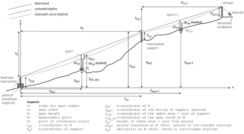
Table 3. Position and properties of the measurement points. x_m: horizontal distance from the head spar to the measurement point [m]; z_m: vertical distance from the bottom of the head spar to the measurement point [m]; z_{ch_m}: vertical distance from the bottom of the head spar to the corresponding height of the span chord at the measurement point [m]; d_{g_ch_m}: distance span-chord to ground [m] (= z_{ch_m –}z_m). BW: Buriwand; KB: Koebelisberg; BL2 and BL3: Banzenloecher Lines 2 and 3

Cable road	Span number	1	2	3
BW	xm [m]	122.50	283.80	365.80
	zm [m]	66.78	177.44	228.59
	zch_m [m]	91.30	192.58	240.22
	dg_ch_m [m]	24.52	15.14	11.63
KB	xm [m]	45.00	207.64
	zm [m]	−22.68	−111.50
	zch_m [m]	−8.27	−69.73
	dg_ch_m [m]	14.41	41.77
BL3	xm [m]	85.40	250.00	406.40
	zm [m]	9.30	45.53	92.87
	zch_m [m]	29.77	70.95	112.95
	dg_ch_m [m]	20.47	25.42	20.08
BL2	xm [m]	130.47	375.71
	zm [m]	11.25	89.44
	zch_m [m]	44.34	106.70
	dg_ch_m [m]	33.09	17.26

Rope and machine properties

Three different tower yarders from the manufacturers Konrad (Konrad Forsttechnik GmbH, Preitenegg, Austria), Koller (Koller GmbH, Schwoich/Kufstein, Austria) and Mayr-Melnhof (MM Forsttechnik GmbH, Frohnleiten Austria) were used. Details on the tower yarders, carriages and ropes can be found in Table 4.

Table 4. Rope and machine properties. BW: Buriwand; KB: Koebelisberg; BL2 and BL3: Banzenloecher Lines 2 and 3

Factor	Unit	BW	KB	BL2	BL3
Yarder type		Syncrofalke – 4 t (Mayr- Melnhof)	KMS 12 (Konrad)	K507 (Koller)	K507 (Koller)
Carriage type		Sherpa U4 XL (Mayr-Melnhof)	Liftliner (Konrad)	Hansliner (in-house construction Abächerli AG)	Skytiger ST 50 (Seik)
Carriage weight	kg	720	790	850	1200
Skyline type		Styria Forst 2 (Haase)	Python Super (Jakob) 8S, 22 mm	Performance, F-30, (Teufelberger) 20.5 mm	Performance, F-30, (Teufelberger) 20.5 mm
Skyline minimum breaking force	kN	430.95	442.80	453.00	453.00
Skyline E-modulus (range, used for sensitivity analysis)	kN mm^−2	100–130	95–105	95–105	95–105
Skyline E-modulus (used for analysis)	kN mm^−2	115	100	100	100
Skyline self-weight	kN m^−1	0.0228	0.0223	0.0205	0.0205
Skyline diameter	mm	22	22	20.5	20.5
Skyline fill factor	[]	0.78	0.68	0.78	0.78
Mainline type		Teufelberger, F20	Teufelberger, FSS 2–619S 3AY, 12 mm	Teufelberger,F-20 (6x25) 12 mm	Teufelberger,F-20 (6x25) 12 mm
Mainline self-weight	kN m^−1	0.0072	0.0074	0.0073	0.0073

Of all the parameters used, the modulus of elasticity (E-modulus) is the parameter with the greatest uncertainty. The E-modulus is a material parameter of the rope, which describes the relationship between the tension and elongation of the rope and shows an S-shaped curve with increasing force application (Feyrer 2015). Therefore, depending on the percentage of the minimum breaking load applied to the rope, the difference in the E-modulus can be large and non-linear. In addition, the E-modulus is dependent on the type of rope. The ISO 12076 (2002) standard therefore recommends that the E-modulus of a specific rope be determined experimentally at a load between 10% and 30% of the minimum breaking force in the entirely settled state (i.e. no additional settlement occurs during a further loading cycle). In this range, the curve is approximately linear. Since an experimental evaluation of the E-modulus was not possible, as part of the rope would have had to be cut out, the rope manufacturers provided us with their value ranges of the E-modulus for the analysis (Table 4). Therefore, a sensitivity analysis of the E-modulus parameter was carried out to quantify the effect of varying this value.

Experimental layout

For the measurements, different load configurations were formed, which were regularly graded and extended up to the maximum recommended payload of the cable yarder. For this purpose, suitable single logs were selected (Figure 2) and composed for the required loads. The single logs were weighed with the scale of a truck crane. The load configuration varied between 7 and 35 kN, including logs and carriage (Table 5).

Figure 2. Weighed logs for load formation at the Buriwand (BW) cable road. The numbers on the logs indicate the weight of the single logs in tons [t]. Please note that both comma and point are used as a decimal point and that the 0.8 is upside-down (reads 8.0 but is 0.8 in reality) (photo: Leo Bont).

Table 5. Load (Q) of different load configurations (LC) at the different test sites. Load configuration LC1 was the carriage only, whereas LC2 to LC4 were composed of the carriage and different log combinations. BW: Buriwand; KB: Koebelisberg; BL2 and BL3: Banzenloecher Lines 2 and 3

Cable road	Carriage (LC1) [kN]	LC2 [kN]	LC3 [kN]	LC4 [kN]
BW	7.06	17.85	26.68	35.02
KB	7.75	18.15	25.41	32.67
BL2	8.34	12.56	19.42	30.31
BL3	11.77	22.66	29.53	33.75

During the measurements, the cable yarder operator was responsible for operating the cable yarder and attaching and detaching the load logs. The researchers had the following tasks: one was responsible for reading the skyline tensile forces on the load cell and another one or two measured the ground clearance at the measurement points. There was radio contact between all people involved.

For every span, the ground clearance at the measurement point and the skyline tensile force were measured simultaneously for each load configuration. For the measurement of the mounting tension (pre-stress tensile force of unloaded skyline) and the ground clearance of the unloaded skyline, the carriage without load was positioned as close as possible to the tower of the yarder (about 1 m distance). For the other measurements, the carriage was stopped at the respective measurement point. In each span, one measurement was carried out with each load configuration. The carriage was not clamped onto the skyline; it was only held in position by the mainline or the haulbackline to eliminate force effects exerted by the mainline or haulbackline on the skyline. The measurement took place when the load of the carriage no longer oscillated.

Please note that the loading conditions between the modeled system and the real system are different. When calculated according to Zweifel (1960), the algorithm incorporates the self-weight of the support ropes (mainline and haulbackline) as an additional weight to the load besides that of the logs. However, it does not consider the loading effect of the support ropes, which means that the support ropes cannot absorb any tensile forces from the carriage. This corresponds to a situation in which the carriage is clamped onto the skyline. In the model, the tensile forces generated by the carriage’s downhill slope force are all conducted to the skyline. The differences between Zweifel’s (1960) assumptions and the measured configuration are visualized in Figure 3. Figure 3A shows Zweifel’s (1960) assumptions, in which the skyline tensile forces and the load Q_Z (carriage weight, load and mainline self-weight for half a span) are included in the equilibrium equation of the carriage. Figure 3B displays the measured situation in which the carriage is held by the mainline. In this case, the skyline and the mainline/haulbackline tensile forces and the load Q_M (carriage-weight and load) are included in the equilibrium equation of the carriage.

Figure 3. Free body diagram of forces acting in the equilibrium equation of the carriage. (A) Situation for the Zweifel (1960) assumptions, in which the carriage is clamped onto the skyline. Zweifel (1960) includes the skyline tensile forces and the load Q_Z (carriage weight, load and mainline self-weight) in the equilibrium equation of the carriage. The equilibrium equation is as follows: Q_Z + V_S,L+ V_S,R = 0 and H_S,L = H_S,R. (B) Measured situation in which the carriage is held by the mainline. In this case, the skyline and the mainline/haulbackline tensile forces and the load Q_M (carriage-weight and load) are included in the equilibrium equation of the carriage. The equilibrium equation is as follows: Q_M + V_S,L+ V_S,R+ V_M,L+ V_M,R = 0 and H_S,L + H_M,L = H_S,R+ H_M,R.V_S: vertical component of the skyline tensile force, V_M: vertical component of the mainline tensile force, H_S: horizontal component of the skyline tensile force, H_M: horizontal component of the mainline tensile force, R: right, L: left.

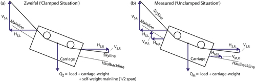
We intentionally measured the situation in which the carriage is not clamped onto the skyline. This verifies the phase of travel of the carriage over one or more spans during which the carriage is not clamped. The carriage is ultimately only clamped during lateral yarding and hooking.

Measurements were started in the span closest to the tower yarder. Then, in each span, all load configurations were tested, starting with the lightest load. When all measurements in one span were completed, the measurements in the next span were carried out. The mounting tension was measured anew each time a switch was made to a new span. The measured mounting tensions are reported in Table 6.

Table 6. Measured mounting tension for each project site. To measure the mounting tension, the unloaded carriage was located 1 m from the tower. The basic skyline tensile force (mounting tension) was measured anew each time a switch was made to a new span

	Measurement place [M = mountain, V = valley]	Mounting tension ($T_{0,E}$) [kN] (measured value of load cell before measurement in span)
Cable road		1	2	3
BW	M	83.48	80.64	79.46
KB	V	88.19	91.72
BL2	M	124.59	120.07
BL3	M	116.54	112.23	110.07

A GoPro camera (GoPro, Inc., San Mateo, CA, USA) was used to observe the yarder tower during the entire measurement period in order to detect any movements of the tower, because even small movements of the tower could violate the basic assumption that a standing skyline has fixed anchors on both ends.

Since the mounting tension was measured at the end point ($T_{0,E}$), the mounting tension at the start point ($T_{0,S}$), which served as input for the calculations, was derived according to Equation 1(1) $T_{0,S}=T_{0,E}-\mathrm{\Delta }{z}_{E,S}\ast q_S$(1) , based on Zweifel (1960). For this purpose, the friction between the jack and skyline was neglected (Zweifel 1960).

(1) $T_{0,S}=T_{0,E}-\mathrm{\Delta }{z}_{E,S}\ast q_S$(1)

with

$q_S$ self-weight of the skyline [kN m⁻¹]

$\mathrm{\Delta }{z}_{E,S}$ difference between z-coordinate of the endpoint and z-coordinate of the start point [m]

Measurement of skyline tensile forces and ground clearance and derivation of deflection

To determine the deflection, which is defined as the vertical distance between the skyline and the chord joining the jacks (cable shoes) of the adjacent supports (or top of the tower), the ground clearance (distance between the ground and the skyline) was measured (Figure 4). The reference point for the skyline was the first wheel on the valley side of the carriage. Based on the ground clearances, the deflections in the individual spans were derived.

Figure 4. Sketch of the measurement layout. The ground clearance is calculated based on the distances and angles to the transponder and the skyline.

A Vertex Laser Geo (Haglöfs, Sweden) was used for the height measurements. The transponder used as a reference point (Figure 4) for the ultrasonic measurement was placed on a tripod directly under the axis of the cable road. All measurements were made by the same person and repeated at least three times. The location for the measurements was chosen to be perpendicular to the course of the cable road. The distance to the cable road was chosen so that the angle relative to the skyline was between 50 g and 70 g, as this range has been demonstrated to yield the most precise measurements (Düggelin and Keller 2017).

The deflection at the measurement point y_m,i was then calculated according Equations 2(2) $y_{m,i}=z_{ch\mathrm{\_}m,i}-g{c}_{m,i}-z_{m,i}$(2) and 3(3) $z_{ch\mathrm{\_}m,i}=z_{cs,i}+h_i\left(\frac{x_{m,i}-x_{s,i}}{w_i}\right)$(3) (see also Figure 1 for an illustration of the variables). As visualized in Figure 1, the variables z and x are aligned in a coordinate system with the origin at the bottom of the head spar, and z can also take negative values for uphill yarding cases.

(2) $y_{m,i}=z_{ch\mathrm{\_}m,i}-g{c}_{m,i}-z_{m,i}$(2)

with

(3) $z_{ch\mathrm{\_}m,i}=z_{cs,i}+h_i\left(\frac{x_{m,i}-x_{s,i}}{w_i}\right)$(3)

$z_{ch\mathrm{\_}m,i}$: z-coordinate of the span chord at the measurement point i [m]

z_m,i: z-coordinate of the measurement point i [m]

x_m,i: horizontal distance from the head spar to the measurement point [m]

w_i: span width [m]

h_i: span height [m]

z_cs,i: z-coordinate of the cable shoe i = z_bs,i + h_s,i [m]

h_s,i: height of cable shoe i from the ground [m]

z_bs,i: z-coordinate of the bottom of the support i [m]

x_s,i: x-coordinate of the cable shoe i = $\sum _i{w}_i$ [m]

gc_m,i: ground clearance at measurement point

Although the deflection at the measurement point y_m,i was not measured directly, but rather derived from the measurement of the ground clearance, we will refer to the measured deflection or absolute measured deflection (AMD = y_m,i), as an approximation for the remainder of the paper.

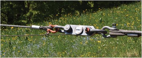
The skyline tensile force was measured at the anchor of the skyline on the opposite side of the tower yarder. For the measurement at the skyline anchor, the load cells (manufactured by PAT Messtechnik AG, Sachseln, Switzerland) were mounted with shackles between the skyline and the anchor (Figure 5). The force was read on an external display box. The load cell is designed to measure tensile forces up to 196 kN and was tested for correctness in the construction laboratory from the Institute of Structural Engineering of ETH Zurich in June 2020.

Figure 5. PAT load cell at the mountain anchor of the Buriwand (BW) cable road (photo: Fritz Frutig).

Mechanical analysis

The deflection and the static skyline tensile forces that occur were calculated according to the approach of Zweifel (Zweifel 1959, 1960). According to that approach, calculations for skyline properties under a load involve three steps:

• Step 1 (unloaded situation): Calculate the unstretched length of the skyline without a load $U_L\left(T_{0,S}\right)$ for a given mounting tension ($T_0$).

• Step 2 (load in the center of span i): Calculate the entire unstretched length of the skyline over all spans under a load at the center of span i $\left(U_{Vi}\right)$ and perform an iterative search for a new mounting tension ${T_{0,Si}}^{\prime }=T_{0,S}+\mathrm{\Delta }{T}_i$ such that $U_L\left(T_{0,S}\right)\approx U_{Vj}\left({T_{0,Si}}^{\prime }\right)$. This step must be repeated for each span i.

• Step 3: Determine the skyline properties under a load (deflection of the load path). It is assumed that the intermediate support is immovable and that no friction exists between the skyline rope and the jack.

For a comparison with the approach usually applied in practice thus far, the deflection according to Pestal (1961) was also computed.

Statistical analysis

To denote the accuracy of the theoretical calculations, we compared the theoretical values with the measured ones. For analyzing the deflection, we mainly used the differences in relative deflection ($\mathrm{\Delta }{y}_{ZM,rel}$) to interpret the results, as described later in the results section. We define the differences in relative deflection according to Equation 4(4) $\mathrm{\Delta }{y}_{ZM,rel}=RTD-RMD$(4) , with the relative measured deflection (RMD) and relative theoretical deflection (RTD) as input (Equations 5(5) $RMD=AMD-AM{D}_{UL}$(5) and 6(6) $RTD=ATD-AT{D}_{UL}$(6) ).

(4) $\mathrm{\Delta }{y}_{ZM,rel}=RTD-RMD$(4)

(5) $RMD=AMD-AM{D}_{UL}$(5)

(6) $RTD=ATD-AT{D}_{UL}$(6)

The measured (AMD), as well as the theoretical (ATD), absolute deflections of the loaded skyline (with the various load configurations) are subtracted from the measured (AMD_UL) or theoretical (ATD_UL) unloaded absolute deflection for this purpose. To analyze the skyline tensile force, the difference between measured and theoretical values ($\mathrm{\Delta }{T}_{ZM}$) is defined in Equation 7(7) $\mathrm{\Delta }{T}_{ZM}=T_{ZT}-T_{MT}$(7) as absolute values [kN] and in Equation 8(8) $\mathrm{\Delta }{T}_{ZM}=\frac{T_{ZT}-T_{MT}}{T_{MT}}\ast 100$(8) as relative values [%]:

(7) $\mathrm{\Delta }{T}_{ZM}=T_{ZT}-T_{MT}$(7)

(8) $\mathrm{\Delta }{T}_{ZM}=\frac{T_{ZT}-T_{MT}}{T_{MT}}\ast 100$(8)

with

T_MT: Skyline tensile force at the top anchor. Measurement value for BW, BL2 and BL3. The value for KB was derived with Equation 1(1) $T_{0,S}=T_{0,E}-\mathrm{\Delta }{z}_{E,S}\ast q_S$(1) from the bottom-anchor measurement.

T_ZT: Theoretical (Zweifel) skyline tensile force at the top anchor.

The following metrics were calculated: root mean square error (RMSE), relative root mean square error (RMSE_P), mean absolute error (MAE) and mean absolute percentage error (MAPE). RMSE was based on a leave-one-out cross-validation and derived according to Equation 9(9) $RMSE=\sqrt{\frac{{\sum }_{x\in s}{\left(\hat{Y}\left(x\right)-Y\left(x\right)\right)}^2}{n}}$(9) .

(9) $RMSE=\sqrt{\frac{{\sum }_{x\in s}{\left(\hat{Y}\left(x\right)-Y\left(x\right)\right)}^2}{n}}$(9)

where $Y\left(x\right)$ is the observed value for one measurement setting $x\in \left(s\right)$ [kN] or [m], $\hat{Y}\left(x\right)$ is the theoretical value for one measurement setting $x\in \left(s\right)$, and s is the dataset composed of n measurement settings.

The relative RMSE, defined as the RMSE relative to the mean y_mean of the observed values, is defined in Equation 10(10) $y_{mean}=\frac{1}{n}\sum _{x\in s}Y\left(x\right)$(10) :

$RMSE\left[\mathrm{\%}\right]=\frac{RMSE}{y_{mean}}\ast 100$, with

(10) $y_{mean}=\frac{1}{n}\sum _{x\in s}Y\left(x\right)$(10)

Further, MAE and MAPE are calculated according to Equations 11(11) $MAE=\frac{1}{n}\sum _{x\in s}\left|\hat{Y}\left(x\right)-Y\left(x\right)\right|$(11) and 12(12) $MAPE\left[\mathrm{\%}\right]=\frac{MAE}{y_{mean}}\ast 100$(12) :

(11) $MAE=\frac{1}{n}\sum _{x\in s}\left|\hat{Y}\left(x\right)-Y\left(x\right)\right|$(11)

(12) $MAPE\left[\mathrm{\%}\right]=\frac{MAE}{y_{mean}}\ast 100$(12)

We further investigated whether the payload, the width or the slope of the span influence the difference between measured and theoretical values. As the observations were clustered we had a single cluster structure, as shown later in the results section; a pure regression was not valid and mixed models (random intercept models) had to be used to account for the non-independent variables. We assumed that there were span-specific effects (caused mainly by measurement inaccuracies and model simplifications), which were introduced as an additional source of variance. The random intercept model is formulated in Equation 13(13) $Y_{ij}\left(x\right)={\beta }_0+{\beta }_1{Z}_{1,ij}+{\beta }_2{Z}_{2,ij}+\dots +{\beta }_p{Z}_{p,ij}+{\epsilon }_{ij}\left(Z\right)+u_j$(13) :

(13) $Y_{ij}\left(x\right)={\beta }_0+{\beta }_1{Z}_{1,ij}+{\beta }_2{Z}_{2,ij}+\dots +{\beta }_p{Z}_{p,ij}+{\epsilon }_{ij}\left(Z\right)+u_j$(13)

with error term ${\epsilon }_{ij}\left(Z\right)\sim N\left(0,{\sigma }_{\epsilon }^2\right)i.i.d.$ and $u_j\sim N\left(0,{\sigma }_u^2\right)i.i.d.$ (j: random effect of the intercept of the j-th span, i: i-th measurement), where $Y_{ij}\left(x\right)$ is the response, ${\beta }_0\dots {\beta }_p$ are the regression coefficients, $Z_{1,ij}\dots Z_{p,ij}$ denote the predictor variables, and p is the number of predictor variables. Due to the relatively small number of observations, we chose a single variance estimate for the random intercept $u_j$. However, to test whether the variance varied by level, we performed an additional ANOVA between the response $Y_{ij}\left(x\right)$ and the j-th span. The analysis was done by applying the lmertest package (Kuznetsova et al. 2017) in R (R Core Team 2021), which also provides p values for the F and t tests. Two random intercept models (rim) were formulated, the first with the response “difference in deflection” ($\mathrm{\Delta }{y}_{ZM,rel}$) [m] (rim #1) and the second with “difference in skyline tensile force” ($\mathrm{\Delta }{T}_{ZM}$) [%] (rim #2), both with the predictors “slope of the span,” “span width” and “load.” A backward stepping approach was used to identify the significant variables. Non-significant variables were removed from the model.

In addition, it was important to determine whether there was a correlation in the differences of the measured and theoretical values between the deflection and the skyline tensile force. For this purpose, a simple linear regression was fitted with the response $\mathrm{\Delta }{T}_{ZM}$ and the predictor $\mathrm{\Delta }{y}_{ZM,rel}$ (lm #1). The R function “lm” was used for this purpose.

Results

A total of 50 settings were monitored and analyzed, including 10 spans in 4 cable roads, with 4 loaded and 1 unloaded configuration in each span. The raw data can be found in the appendix (Table A1).

Skyline tensile forces

Figure 6A illustrates the measured skyline tensile force (measured at the top-anchor with the load at the measurement point). The skyline tensile force increased with heavier loads and longer cable spans and even achieved double the value of the mounting tension force of the unloaded skyline, as seen for span 1 in BW, where an increase from 77.8 kN to 154.0 kN was observed.

Figure 6. (A) Measured skyline tensile forces (T_MT) in the cable roads and spans for the different load configurations. The bottom end of each line indicates the mounting tension/pre-stress tensile force. (B) Absolute measured deflection (AMD) of the skyline [m], derived from the measured ground clearance, for the different load configurations and the respective spans. Cable road abbreviations: BW: Buriwand, KB: Koebelisberg, BL2 and BL3: Banzenloecher Lines 2 and 3.

The differences between measured and theoretical (Zweifel) skyline tensile forces ($\mathrm{\Delta }{T}_{ZM}$) are displayed in Figure 7A and the corresponding metrics are given in Table 7. The differences amounted to a mean absolute percentage error (MAPE) of 3.2% or a root mean square error (RMSE) of 6.7%. Larger deviations of more than 3.5% occurred in the long spans (span width > 100 m) of the steep cable roads of BW and KB only (Figure 7A). In these cases (BW span 1, KB span 2), the cable tensile forces were always overestimated when the approach of Zweifel (1960) was applied, with a maximum value of up to 12.7% for the heaviest load configuration. In this most extreme case (BW span 1), the measured skyline tensile force was 154.0 kN, whereas the computed tensile force was 173.6 kN (+ 12.7%).

Figure 7. (A) Differences between the measured skyline tensile force and the theoretical values (ΔT_ZM) [%]. The measured value serves as a reference. A positive ΔT value means that the theoretical skyline tensile forces are higher than the measured ones. Only loaded skyline configurations are displayed. (B) Differences between the theoretical (RTD) and the measured relative (RMD) skyline deflection for loaded situations (Δy_ZM,rel) [m]. A positive value means that the theoretical deflection values are higher than the measured ones. Cable road abbreviations: BW: Buriwand, KB: Koebelisberg, BL2 and BL3: Banzenloecher Lines 2 and 3.

Table 7. Root mean square error (RMSE), mean absolute error (MAE), mean absolute percentage error (MAPE) and root mean square error in percent (RMSE_P) for the skyline tensile force calculations compared with the measured values. The metrics were computed for each cable road separately and for all cable roads together (overall)

Cable road	RMSE [kN]	MAE [kN]	MAPE [%]	RMSE_P [%]
BL2	1.45	1.13	0.69	0.87
BL3	3.02	2.71	1.82	2.01
BW	8.25	5.86	4.65	6.07
KB	10.6	8.1	5.9	7.4
Overall	6.75	4.39	3.22	4.78

In the cable roads BL2 and BL3, with “moderate” steepness, the average deviations were only 1.3% (MAPE) and 1.4% (RMSE), respectively, while the approach of Zweifel (1960) slightly underestimated the cable tensile forces, with a maximum underestimation of 3.5% in span 3 of cable road BL3.

In Figure 8A, the differences of the skyline tensile forces ($\mathrm{\Delta }{T}_{ZM}$) are compared with the slope of a span. Our first impression was that with an increasing slope of a span, the skyline tensile force was overestimated by the theoretical computation (Zweifel). However, this trend was not statistically significant over all observations, indicated by the random intercept model #2 (rim #2) (see Appendix for the complete model output, ANOVA table and residual plot, Figure A2,A4), which only showed a significant influence of the payload (p-value = 0.00047) on the differences in the skyline tensile forces ($\mathrm{\Delta }{T}_{ZM}$) between measured and theoretical values.

Figure 8. (A) Comparison of the differences in the skyline tensile forces (ΔT_ZM) [%] (theoretical vs. measured) and (B) the relative difference in deflection (Δy_ZM,rel) [m] (theoretical vs. measured) compared with the slope for each span. Cable road abbreviations: BW: Buriwand, KB: Koebelisberg, BL2 and BL3: Banzenloecher Lines 2 and 3.

Skyline tensile forces according to Pestal (1961) were not computed, as this method does not make any statements about the skyline tensile forces that occur. Its basic assumption is that the horizontal force component does not change when the carriage passes over a span.

Deflection

The results of the deflection measurements (AMD) for all spans and load configurations are shown in Figure 6B. The deflection increased with heavier loads and longer spans. The largest measured deflections were found with the heaviest load configurations in span 1 for cable roads BW and BL2 and in span 2 for KB. Surprisingly, we found a negative deflection in span 2 of BW.

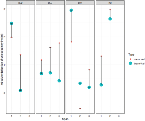
A comparison of the measured and theoretical absolute deflections showed that there were differences between measured and theoretical deflections already in the unloaded case (Figure 9). In our opinion, these differences in the unloaded deflection were also caused by measurement inaccuracies. The Vertex measurements of the jack/cable shoe heights, the GPS height measurements at the bottom end of the supports and at the measurement points, and the Vertex measurements (distance from ground to skyline) at the measurement points are included in the calculation of the absolute measured deflection. All these measurements are subject to inaccuracies that can accumulate. In our experience, erroneous GPS signals in particular are a major source of error. Although differential GNSS (dGNSS) receivers were used, positional errors must still be expected under a closed canopy (Lamprecht et al. 2017). These devices account for atmospheric diffraction effects, but precise measurements require a logging time of approximately 20 minutes (Naesset and Jonmeister 2002; Hauglin et al. 2014). According to the same authors, however, the measured dGNSS positional errors still vary between 0.49 and 3.60 m for basal areas (BAs) below 30 m² ha⁻¹ and between 2.15 and 5.60 m for BAs above 45 m² ha⁻¹.

Figure 9. Deflection of the unloaded skyline. Comparison of absolute measured deflection (AMD) and absolute theoretical deflection (ATD). Cable road abbreviations: BW: Buriwand, KB: Koebelisberg, BL2 and BL3: Banzenloecher Lines 2 and 3.

For the reasons mentioned above, we used the differences in relative deflection to interpret the results ($\mathrm{\Delta }{y}_{ZM,rel}$), according to Equation 4(4) $\mathrm{\Delta }{y}_{ZM,rel}=RTD-RMD$(4) . Thus, we eliminated the inaccuracies in measuring the support heights and all z-coordinates (vertical-coordinates), except for the Vertex measurement of the ground clearance. Inaccuracies related to the measured x-coordinates (horizontal coordinates), however, still remained.

The differences between measured and theoretical relative deflections ($\mathrm{\Delta }{y}_{ZM,rel}$) were between +0.9 m and −0.73 m (Figure 7B), where a + sign means that the theoretical relative deflection was larger than the measured one, or, in other words, that the deflection was overestimated when applying the approach of Zweifel (1960) (the measured value always serves as a reference). Overall, there were equal numbers of spans in which the deflection was overestimated or underestimated in the calculation (five in each case). The difference was most pronounced for the heavy loads. For practical applications, the large spans were of particular interest, since large and relevant deflections occurred in these spans (BL2: 1; BL3: 1, 2, 3; BW: 1; KB: 2). Looking only at these spans with horizontal lengths greater than 100 m, a slight underestimation was found in the “steep” spans of BW and KB and a slight overestimation in the spans of BL2 and BL3 with “moderate” steepness, again with differences having a range of +0.9 m to −0.73 m (Figure 6B).

Table 8 shows the corresponding metrics for $\mathrm{\Delta }{y}_{ZM,rel}$. The MAE amounted to 0.39 m and the RMSE to 0.47 m over all spans, and the best accuracy occurred in cable road BW, with a MAE of 0.25 m and a RMSE of 0.31 m. The “worst values” corresponded to the cable road KB, with a MAE of 0.55 m and a RMSE of 0.6 m (Figure 7B).

Table 8. Root mean square error (RMSE), mean absolute error (MAE), mean absolute percentage error (MAPE) and root mean square error in percent (RMSE_P) for the deflection calculations compared with the measured values. The metrics were computed for each cable road separately and for all cable roads together

Cable road	RMSE [m]	MAE [m]	MAPE [%]	RMSE_P [%]
BL2	0.32	0.26	4.89	5.42
BL3	0.56	0.49	7.48	8.64
BW	0.31	0.25	4.96	7.22
KB	0.60	0.55	8.99	10.49
Overall	0.47	0.39	6.55	8.14

In Figure 8B, the differences in relative deflections ($\mathrm{\Delta }{y}_{ZM,rel}$) are compared with the slope of a span. As a first impression, a slight trend was observed that is similar to the behavior of the skyline tensile force: with increasing slope of a span, the deflection tended to be underestimated by the theoretical computation (Zweifel). However, this trend was not significant and, consequently, “slope” was removed as a predictor from the fitted random intercept model #1 (rim #1) (see Appendix for the complete model output, ANOVA table and residual plot, Figure A1,A3). On the other hand, there was a significant influence of the load, with a p-value of 0.00247, as was already the case for the skyline tensile force.

Figure 10 shows the relationship between differences in the skyline tensile forces ($\mathrm{\Delta }{T}_{ZM}$) and deflection ($\mathrm{\Delta }{y}_{ZM,rel}$) (lm #1). As we had clustered data, the relationships were plotted and analyzed for each cable road separately. A clear and significant correlation (p-value = 0.003) was only identified for KB, with an R_adj value of 0.75 (see also model outputs in the Appendix, Figure A5). For BW, BL2 and BL3, the response ($\mathrm{\Delta }{T}_{ZM}$) was independent of the deflection ($\mathrm{\Delta }{y}_{ZM,rel}$). An overestimation of the skyline tensile forces was observed in only one cable road, with an underestimation of the deflection.

Figure 10. Comparison of the differences in the skyline tensile forces (ΔT_ZM) [%] (theoretical vs. measured) and the relative difference in deflection (Δy_ZM,rel) [m] (theoretical vs. measured) with regression line for each cable road. Cable road abbreviations: BW: Buriwand, KB: Koebelisberg, BL2 and BL3: Banzenloecher Lines 2 and 3.

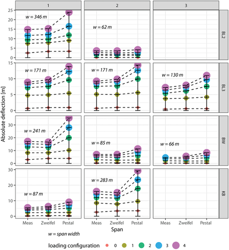
Figure 11 depicts the absolute deflections of the loaded and unloaded skyline for the approaches of Zweifel (1960) and Pestal (1961), as well as for the measured values. The theoretical deflections according to Zweifel (1960) were smaller than those according to Pestal (1961). The difference between the two methods increased with heavier loads and longer spans. The approach of Zweifel (1960) led to more realistic results.

Figure 11. Absolute deflections for the loaded (loading configurations 1–4) and the unloaded skyline (loading configuration 0) for the approaches of Zweifel (1960) and Pestal (1961) and for the measured values (Meas). Cable road abbreviations: BW: Buriwand, KB: Koebelisberg, BL2 and BL3: Banzenloecher Lines 2 and 3.

Sensitivity analysis of the E-modulus

Figure 12 shows the influence of the uncertainty in the E-modulus on the results. For each span and load configuration, a range from the lowest (95 kN mm⁻² for BL2, BL3 and KB; 100 kN mm⁻² for BW) to the highest E-modulus (105; 130 kN mm⁻²) was displayed. For both tensile force and deflection, the range increased with heavier loads and longer span widths. By visualizing the skyline tensile force (Figure 12A), we noticed that the resulting uncertainty range caused by the E-modulus had approximately the same magnitude as the difference between measured and theoretical values. However, we also observed that the clear overestimation of the skyline tensile force in the spans of cable roads BW and KB, which was already observed earlier, was not caused by the E-modulus alone. By looking more closely at Figure 12B, where the deflection is depicted, one can see that the overestimation of the deflection in cable roads (BL2 and BL3 all spans, KB span 1) did not change much with variation in the E-modulus. The underestimation of the deflection in BW span 1 could instead be caused by an inaccurate E-modulus.

Figure 12. Sensitivity analysis for varying E-modulus (displayed for all load configurations). (A) Range for the difference between theoretical and measured skyline tensile force (ΔT_ZM) [%]. (B) Range for the relative difference between theoretical and measured deflection (Δy_ZM,rel) [m]. In A, the upper bound of the “error bar” represents the highest E-modulus (105 for BL2, BL3 and KB; 130 for BW) [kN mm⁻²], whereas the lower bound represents the lowest E-modulus (95; 100) [kN mm⁻²]. The point in the center indicates the mean of the range (100; 115) [kN mm⁻²]. In B, the displayed E-modulus values are exactly the other way around: the upper bound of the “error bar” represents the lowest E-modulus. Cable road abbreviations: BW: Buriwand, KB: Koebelisberg, BL2 and BL3: Banzenloecher Lines 2 and 3.

Discussion

Accuracy of deflection and tensile force predictions

The skyline tensile force was predicted with an accuracy of 5.35 % or 7.43 kN (both RMSE), and all values were within a range of −3.5% to +12.7% deviation from the measured values. The prediction was better in flat spans than in steep spans. In the latter, a clear overestimation of the predicted tensile force was observed, which could not be explained by variation in E-modulus alone. The RMSE between measured and predicted deflection was 0.47 m, or 8.14%, and the MAE was 0.39 m. All predicted values were within a range of deviation of −0.73 m to +0.9 m, taking the measurements as a reference.

The results (RMSE) can only be compared with caution with the findings of Dupire et al. (2016), since other span configurations (flatter and fewer spans) and, most importantly, much heavier load configurations were used in our study. However, our results are consistent with the previous findings. Dupire et al. (2016) report RMSE values of 0.15 m to 0.44 m for the prediction of the entire load path and 1 to 2 kN for the skyline tensile forces. In contrast to our results, Dupire’s RMSE is based not only on values in the mid-span, but also on values along the entire span. Thus, it also contains values from locations that are very close to the supports and consequently do not show large variation by design.

Uncertainties and their impact on the results

Several aspects had an influence on the accuracy of our results:

• Mechanical assumptions: the friction between the skyline and the jack is not considered in the approach of Zweifel (1960). Furthermore, the aspect of the loading of the support ropes (mainline and haulbackline) is not considered. Additionally, the anchors at both ends are not entirely fixed in reality, as assumed, and the intermediate support trees likewise are not completely fixed elements.

• Measurement inaccuracies: inaccuracies occur, in particular for the measurement of the deflection. The exact determination of the absolute deflection, taking the span chord as a reference, is rather difficult. Therefore, we used the relative differences in the deflection measurements, taking the unloaded situation as a reference, to interpret the results. However, measurement errors could still have occurred.

• Imprecise parameters, such as the E-modulus and the load weight, can influence the accuracy.

The only relevant deviation from the model predictions was the observed overestimation of the skyline tensile force in the steep and long spans (BW span 1, KB span 2). However, across all observations in all spans, this observation was statistically not significant. Simultaneously, we found that this overestimation of the tensile forces was not correlated with an over or underestimation of the deflection, although this was observed in cable road KB. As shown by Dupire et al. (2016), neglecting the effect of the loading of the mainline leads to a higher modeled tensile force in the skyline in steep spans. This can be explained by the fact that in a steep span, the load hangs more on the mainline, which takes some of the load of the carriage off the skyline. The steeper the span, the greater the effect. This is one obvious explanation for the observed overestimation of the skyline tensile forces in the steep spans. Furthermore, neglecting the effect of the friction between the skyline and jack at the intermediate supports in the model leads to higher modeled tensile forces in the skyline, as shown by Dupire et al. (2016). This behavior can be explained by the fact that the friction on the supports absorbs part of the tensile force.

As mentioned above, there was no significant relationship between the overestimation of the skyline tensile force and an over or underestimation of the deflection over all spans. For this relationship, several superimposed effects can play a role, which can also have opposing effects or even cancel each other out, which makes an exact analysis challenging. For example, the higher the tensile force, the lower the deflection should be. If the tensile force is overestimated, then the deflection should be underestimated. Another effect to consider concerning this relationship is the fact that the maximum deflection in steep spans does not occur at mid-span (as assumed by Zweifel), but is shifted somewhat upslope (Dupire et al. 2016; Knobloch and Bont 2021). Further influencing factors, such as the friction between the skyline and jack, are mentioned at the beginning of this section.

In addition, we observed a certain variance in the differences between the measurements and the theoretical calculations (for both tensile forces and deflection), which may be caused by several superimposed effects: (1) elastic anchors that are not completely fixed result in a configuration that behaves similar to shorter spans, but with the same unstretched skyline length. Therefore, based on this effect, one would expect larger deflections and smaller skyline tensile forces in reality than predicted by the model. Since each anchor behaves independently, this may explain some of the variance. (2) The not entirely accurate value of the E-modulus can also explain part of the variance in the values, both in the deflection and in the tensile forces. In deflection, the E-modulus leads to an uncertainty range of ± 20 cm, but in some cases it can be up to ± 50 cm. (3) Measurement inaccuracies also contribute to the variation.

Comparison of the approaches of Zweifel and Pestal

The deflections were considerably overestimated with the approach of Pestal (1961), especially for heavy loads and long spans. These situations are particularly important for the design of cable roads. For shorter spans, the differences are not as pronounced. We therefore do not recommend the use of the approach of Pestal (1961) for the design of long cable roads.

Significance of the results for practice

The results of this study are of high practical relevance. Provided that a proper set-up is carried out, the model assumptions (fixed skyline anchors at both ends) are valid and reasonable results can be achieved even with larger, realistic load configurations.

The model predictions agree well with reality and appear to be sufficiently accurate for practical purposes and without systematic bias. For the deflection, an accuracy of about one meter can be expected. This statement is based on the analysis of relative deflections, for which we found the deviations between the measured and theoretical values to be between −0.73 and 0.9 m. In steep spans, the static skyline tensile force is overestimated in the model. It must be noted that we measured the case in which the carriage is not clamped onto the skyline but is held by the mainline or haulbackline. We assume that if the carriage is clamped onto the skyline (such as during hook and lateral yarding), the skyline tensile force is no longer overestimated by the model. The unclamped carriage would lead to a lower skyline tensile force than for the clamped carriage, as the clamped carriage would no longer be held entirely by the mainline. This means that, for the clamped situation, the tensile force in the mainline decreases and shifts to the skyline, in which it increases.

As mentioned above, a limitation of the implemented approach of Zweifel (1960) is that it does not consider the mainline loading, in particular for steep spans. However, the use of more accurate methods, such as that of Dupire et al. (2016), would require additional input parameters that are difficult to gather, such as the angle between the skyline and the mainline at the carriage.

Limitations

A limitation of this study is the rather small number of measurements: 50 settings were monitored and analyzed, composed of 10 spans in 4 cable roads. In order to make more precise statistical statements, we therefore recommend carrying out further measurements of deflections and skyline tensile forces.

Outlook

For future field acquisitions, we recommend that a wide range of situations be covered. As mentioned by Dupire et al. (2016), we also recommend that further experimental measurements concern the friction at the intermediate supports and the variation in tension caused by partial suspension of the logs. For this purpose, it would be helpful to measure skyline tensile forces not only at one end of the skyline, but at both ends. Further, it would be interesting to measure and compare the forces and deflections for different carriage connections to the skyline (clamped, held only at the mainline).

It also became apparent during our study that accurate measurements of the spans, especially the deflection measurement, are a challenge. The method presented by Dupire et al. (2016), with a total station and a sensor on the carriage, is certainly accurate but has been found to be impractical for long multi-span configurations. Also, GPS measurements are not sufficiently accurate in the forest. With our method, we think that the absolute values might be subject to errors but that the relative values are more reliable. Finally, it would be advantageous to have a method for measuring absolute deflection with high precision.

Acknowledgements

We are very grateful to the Federal Office for the Environment (FOEN), the Swiss Forest and Wood Research Fund (WHFF-CH), and the professorship of Prof. Dr. H.R. Heinimann (ETHZ) for the financial support of this project. We also thank the forest contractors Nüesch und Ammann AG (Eschenbach SG) and Abächerli Forstunternehmen AG (Giswil OW) for dedicated cooperation during the measurements and for the testing of Seilaplan in daily business, the forest enterprise Tössstock (state forest Zurich) and Ortsgemeinde Lichtensteig for the permission to carry out measurements at their sites, and the forestry company Untervaz GR for constructive feedback on Seilaplan. We further thank Pfeifer Isofer AG for valuable input on cable properties and for the loan of a load cell, the forestry company Mayr-Melnhof for information on the cable equipment and for testing the measurement protocol during an internship, and Wyssen Seilbahnen AG (Reichenbach BE) for answering our questions about support saddles, cable properties and cable yarders. We are grateful to Roxana Zehtabchi and Marielle Fraefel for field measurement assistance. Last but not least, we thank Melissa Dawes for English editing assistance.

Disclosure statement

No potential conflict of interest was reported by the author(s).

Additional information

Funding

This research was partially funded by the Swiss Forest and Wood Research Fund (WHFF-CH) [Project 2019.04].

Appendix

Software Installation (Seilaplan)

Seilaplan can be installed via the QGIS plugin menu under Plugins > Manage and Install Plugins. A new repository must be added under Settings. The address of the repository is: https://raw.githubusercontent.com/piMoll/SEILAPLAN/master/plugin.xml

The plugin can be installed under version 3.6 or newer of QGIS, but updating to a current version of QGIS is advised. To let QGIS automatically check for plugin updates, the corresponding setting under Manage and Install Plugins > Settings has to be activated. Whenever an update for a plugin is available, a notification will appear at the bottom of the QGIS interface.

The plugin supports four languages: German, French, Italian and English. Seilaplan automatically adopts the language settings of QGIS (Settings > Options > General > Locale menu). If the language of QGIS cannot be adopted, Seilaplan will be displayed in English. To change the language of the plugin manually, the language settings in QGIS have to be adjusted and then QGIS has to be restarted.

Software availability (Seilaplan)

Name of software: Seilaplan

Software required: QGIS 3.6 or newer

Program language: Python 3

Developers: Leo Bont (cable mechanics, optimization), Patricia Moll (GUI),

Software license: GNU – General Public License

Contact address: Sustainable Forestry Group, Swiss Federal Institute for Forest, Snow and Landscape Research (WSL), Zuercherstrasse 111, CH 8903 Birmensdorf, Switzerland

E-Mail: [email protected]

Availability: https://seilaplan.wsl.ch/ (website, documentation) or http://pimoll.github.io/SEILAPLAN/ (source code)

Table A1:

Raw Data

Raw measurement data. The deflection measurement data were derived from ground clearance measurements; (* = not measured at top-anchor, derived from bottom-anchor measured value according to Equation 1(1) $T_{0,S}=T_{0,E}-\mathrm{\Delta }{z}_{E,S}\ast q_S$(1) )

					Skyline tensile force			Deflection (difference from span chord to skyline at measurement point)
Cable road	Span	Load configuration	Load (Q)	Mounting tension (T_0,S)	Zweifel (top-anchor, TZT)	Meas. (top-anchor, TMT)	Meas. (bottom-anchor)	Zweifel (ATD)	Pestal	Meas. (AMD)	Zweifel/Pestal (unloaded skyline)(ATDUL)	Measured (unloaded skyline) (AMDUL)
			[kN]	[kN]	[kN]	[kN]		[m]	[m]	[m]	[m]	[m]
BW	1	1	7.063	77.82	102.67	100.16		8.26	10.25	7.12	2.95	1.82
BW	1	2	17.85	77.82	131.92	123.90		12.42	19.98	11.72	2.95	1.82
BW	1	3	26.68	77.82	154.11	141.26		14.81	27.94	14.22	2.95	1.82
BW	1	4	35.02	77.82	173.61	154.02		16.63	35.46	16.02	2.95	1.82
BW	2	1	7.063	74.98	86.39	86.82		2.47	2.65	1.94	0.35	−0.56
BW	2	2	17.85	74.98	102.33	101.04		4.70	5.99	4.04	0.35	−0.56
BW	2	3	26.68	74.98	116.51	115.56		6.01	8.73	5.24	0.35	−0.56
BW	2	4	35.02	74.98	129.70	122.63		6.98	11.32	6.04	0.35	−0.56
BW	3	1	7.063	73.80	83.71	83.48		1.80	1.89	2.73	0.20	0.83
BW	3	2	17.85	73.80	96.84	93.20		3.61	4.38	4.23	0.20	0.83
BW	3	3	26.68	73.80	109.27	101.34		4.70	6.42	5.23	0.20	0.83
BW	3	4	35.02	73.80	120.96			5.53	8.34		0.20	0.83
KB	1	1	7.75	91.30	96.68	98.27*	95.16	2.31	2.45	3.31	0.29	1.31
KB	1	2	18.15	91.30	110.61	112.98*	109.87	4.30	5.21	4.91	0.29	1.31
KB	1	3	25.41	91.30	121.61	123.09*	119.98	5.36	7.15	5.61	0.29	1.31
KB	1	4	32.67	91.30	132.68	135.54*	132.44	6.24	9.08	6.51	0.29	1.31
KB	2	1	7.75	94.83	116.27	109.06*	105.95	7.85	9.63	8.87	2.64	2.97
KB	2	2	18.15	94.83	145.15	131.62*	128.51	11.65	17.83	12.37	2.64	2.97
KB	2	3	25.41	94.83	164.33	146.34*	143.23	13.59	23.55	14.57	2.64	2.97
KB	2	4	32.67	94.83	182.46	164.48*	161.37	15.21	29.28	16.27	2.64	2.97
BL2	1	1	8.339	122.48	143.23	145.19		7.90	9.02	6.99	2.48	1.99
BL2	1	2	12.56	122.48	153.73	155.19		9.72	11.89	8.89	2.48	1.99
BL2	1	3	19.42	122.48	171.23	173.64		12.18	16.55	11.19	2.48	1.99
BL2	1	4	30.31	122.48	198.36	196.20		15.26	23.94	14.29	2.48	1.99
BL2	2	1	8.339	117.97	122.34	122.43		1.21	1.23	2.56	0.09	1.36
BL2	2	2	12.56	117.97	124.84	124.59		1.73	1.80	2.96	0.09	1.36
BL2	2	3	19.42	117.97	130.03	129.88		2.51	2.71	3.96	0.09	1.36
BL2	2	4	30.31	117.97	140.34	139.79		3.57	4.17	4.86	0.09	1.36
BL3	1	1	11.77	114.09	129.02	130.08		4.91	5.44	5.27	0.69	1.17
BL3	1	2	22.66	114.09	146.83	148.33		7.60	9.61	7.67	0.69	1.17
BL3	1	3	29.53	114.09	158.64	160.69		8.95	12.23	8.77	0.69	1.17
BL3	1	4	33.75	114.09	165.89	166.77		9.68	13.85	9.37	0.69	1.17
BL3	2	1	11.77	109.77	125.26	128.51		5.03	5.62	6.02	0.71	1.62
BL3	2	2	22.66	109.77	143.51	147.15		7.75	9.92	8.52	0.71	1.62
BL3	2	3	29.53	109.77	155.45	158.92		9.10	12.63	9.52	0.71	1.62
BL3	2	4	33.75	109.77	162.76	166.77		9.84	14.30	10.12	0.71	1.62
BL3	3	1	11.77	107.61	119.98	121.64		3.87	4.22	5.08	0.43	1.78
BL3	3	2	22.66	107.61	135.29	137.34		6.17	7.59	6.78	0.43	1.78
BL3	3	3	29.53	107.61	145.73	149.11		7.33	9.71	7.78	0.43	1.78
BL3	3	4	33.75	107.61	152.17	157.74		7.96	11.01	8.58	0.43	1.78

Model outputs

Figure A1. Residual plot for the random intercept model #1 (rim #1).

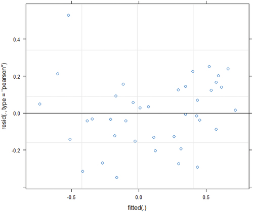
Figure A2. Residual plot for the random intercept model #2 (rim #2).

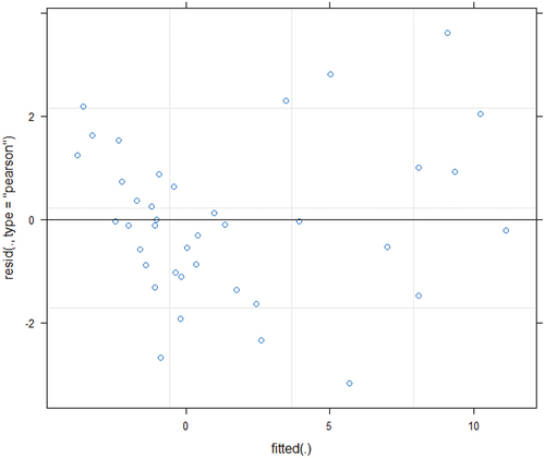
Figure A3. R command and summary model output for the random intercept model 1 (rim #1).Variables: y_norm_Delta: ‘difference in relative deflection’ (RTD - RMD) [m]; delta_T_perc: ‘diff. in skyline tensile force (STF)’(theor. STF – meas. STF) / meas. STF * 100 [%]; slope: ‘slope of the span’ []; Span_Width: ‘spanwidth’ [m]; Q:‘load’ [kN].

Figure A4. R command and summary model output for the random intercept model 2 (rim #2).

Figure A5. R command and summary model output for the simple linear regression model (lm #1).

References

- Bont L, Heinimann HR. 2012. Optimum geometric layout of a single cable road. Eur J Forest Res. 131(5):1439–1448. doi:10.1007/s10342-012-0612-y.
- Bont LG, Church RL. 2018. Location set-covering inspired models for designing harvesting and cable road layouts. Eur J For Res. 137(6):771–792. doi:10.1007/s10342-018-1139-7.
- Bont LG, Moll PE, Ramstein L, Frutig F, Heinimann HR, Schweier J. 2022. SEILAPLAN, a QGIS plugin for cable road layout design. Croat J For Eng.
- Carson WW. 1973. Dynamic characteristics of skyline logging cable systems [PhD Thesis]. University of Washington, Mechanical Engineering.
- Carson WW, Mann CN. 1970. A technique for the solution of skyline catenary equations. Portland (Oregon): USDA For.Serv.Res.Pap. PNW–110. 18.
- Düggelin C, Keller M. 2017. Schweizerisches Landesforstinventar. Feldaufnahme-Anleitung 2017. Birmensdorf (Switzerland): Eidg. Forschungsanstalt für Wald, Schnee und Landschaft WSL.
- Dupire S, Bourrier F, Berger F. 2016. Predicting load path and tensile forces during cable yarding operations on steep terrain. J For Res. 21:1–14. doi:10.1007/s10310-015-0503-4.
- Erber G, Spinelli R. 2020. Timber extraction by cable yarding on flat and wet terrain: a survey of cable yarder manufacturer’s experience. Silva Fenn. 54:20. doi:10.14214/sf.10211.
- Fabiano F, Marchi E, Neri F, Piegai F 2011. Skyline tension analysis in yarding operation: case studies in Italy. Pushing the boundaries with research and innovation in forest engineering. FORMEC 2011, Proceedings of the 44th International Symposium on Forestry Mechanisation; Graz, Austria: Citeseer, p. 9–13.
- Feyrer K. 2015. Wire ropes under tensile load. In: Feyrer K, editor. Wire ropes: tension, endurance, reliability. Berlin (Heidelberg): Springer; p. 59–177.
- Hauglin M, Lien V, Næsset E, Gobakken T. 2014. Geo-referencing forest field plots by co-registration of terrestrial and airborne laser scanning data. Int J Remote Sens. 35(9):3135–3149. doi:10.1080/01431161.2014.903440.
- Heinimann HR. 2003. Holzerntetechnik zur Sicherstellung einer minimalen Schutzwaldpflege: Bericht im Auftrag des Bundesamtes für Umwelt, Wald und Landschaft (BUWAL). Interner Bericht/ETH For Eng. 12:53.
- Heinimann HR, Stampfer K, Loschek J, Caminada L. 2006. Stand und Entwicklungsmöglichkeiten der Mitteleuropäischen Seilkrantechnik - Perspectives on Central European Cable Yarding Systems. Austrian J For Sci. 123:121–139.
- Irvine MH. 1981. Cable structures. Cambridge: The MIT Press. 259.
- Kendrick D, Sessions J. 1991. A solution procedure for calculating the standing skyline load path for partial and full suspension. For Prod J. 41:57–60.
- Knobloch C, Bont LG. 2021. A new method to compute mechanical properties of a standing skyline for cable yarding. PLoS ONE. 16:e0256374. doi:10.1371/journal.pone.0256374
- Kuznetsova A, Brockhoff PB, Christensen RHB. 2017. lmerTest Package: tests in Linear Mixed Effects Models. J Stat Softw. 82:1–26. doi:10.18637/jss.v082.i13
- Lamprecht S, Hill A, Stoffels J, Udelhoven T. 2017. A machine learning method for co-registration and individual tree matching of forest inventory and airborne laser scanning data. Remote Sens. 9(5):505. doi:10.3390/rs9050505.
- Mancuso A, Belart F, Leshchinsky B. 2018. Operative loading in cable yarding systems: field observations of static and dynamic tensions in mobile anchor systems. Can J For Res. 48:1406–1410. doi:10.1139/cjfr-2018-0219
- Mologni O, Lyons CK, Zambon G, Proto AR, Zimbalatti G, Cavalli R, Grigolato S. 2019. Skyline tensile force monitoring of mobile tower yarders operating in the Italian Alps. Eur J Forest Res. 138(5):847–862. doi:10.1007/s10342-019-01207-0.
- Mologni O, Marchi L, Lyons KC, Grigolato S, Cavalli R, Röser D. 2021. Skyline tensile forces in cable logging: field observations vs. software calculations. Croat J For Eng. 42(2):227–243. doi:10.5552/crojfe.2021.722.
- Naesset E, Jonmeister T. 2002. Assessing point accuracy of DGPS under forest canopy before data acquisition, in the field and after postprocessing. Scand J For Res. 17(4):351–358. doi:10.1080/02827580260138099.
- Pestal E. 1961. Seilbahnen und Seilkräne für Holz- und Materialtransporte. Wien und München: Georg Fromme & Co.
- Pyles MR, Anderson JW, Stafford SG. 1991. Capacity of second-growth douglas-fir and Western Hemlock stump anchors for cable logging. J For Eng. 3:29–37. doi:10.1080/08435243.1991.10702631
- R Core Team. 2021. R: a language and environment for statistical computing. Vienna (Austria): R Foundation for Statistical Computing. https://www.R-project.org/.
- Schweier J, Klein M-L, Kirsten H, Jaeger D, Brieger F, Sauter UH. 2020. Productivity and cost analysis of tower yarder systems using the Koller 507 and the Valentini 400 in southwest Germany. Int J For Eng. 31(3):172–183. doi:10.1080/14942119.2020.1761746.
- Schweier J, Ludowicy C. 2020. Comparison of a cable-based and a ground-based system in flat and soil-sensitive area: a case study from Southern Baden in Germany. Forests. 11:611. doi:10.3390/f11060611
- Sessions J. 1976. Field measurement of cable tensions for skyline logging systems. Corvallis OR (USA): Forest Research Laboratory, School of Forestry, Oregon State University.
- Spinelli R, Magagnotti N, Cosola G, Grigolato S, Marchi L, Proto AR, Labelle ER, Visser R, Erber G. 2021. Skyline tension and dynamic loading for cable yarding comparing conventional single-hitch versus horizontal double-hitch suspension carriages. Int J For Eng. 32(sup1):31–41. doi:10.1080/14942119.2021.1909322.
- Visser R. 1998. Tensions monitoring of forestry cable systems [PhD Thesis]. BOKU. Vienna
- Visser R, Harrill H. 2017. Cable yarding in North America and New Zealand: a review of developments and practices. Croat J For Eng. 38:209–217.
- Zweifel O. 1960. Seilbahnberechnung bei beidseitig verankerten Tragseilen. Schweiz Bauztg. 78:11.
- Zweifel O. 1959. Näherungslösungen für die Lastwegkurve einer Einzellast bei beidseitiger Verankerung der Tragseile. Int Seilbahn Rundsch. 2:8.