A multi-objective optimization strategy for timber forwarding in cut-to-length harvesting operations

ABSTRACT

Optimization of forwarding work on the trail network created by the harvester in cut-to-length operations carries much potential for increasing the efficiency and reducing the environmental impact of timber removal. While several approaches to this optimization task have been proposed, existing methods focus on optimizing a single objective at a time. In this work, a heuristic multi-objective optimization strategy for the problem is presented, where the route length, operation duration, and soil damage can be optimized simultaneously. The strategy is based on a tailored version of ant colony optimization and linear scalarization of the full multi-objective problem. The relative importance of the objectives can be set via tunable weights, and the approach is of a modular nature. Results on a realistically sized clearcut harvest site indicate that the strategy produces promising results and gives the expected qualitative behavior when optimizing either a single objective or two objectives at a time.

KEYWORDS:

• Forest machine route optimization
• ant colony optimization
• forwarding productivity
• sustainable forestry

Introduction

Timber removals are increasing globally, as demand for wood products escalates due to growing populations and incomes (FAO 2020). Wood products also have a key role in strategies for transitioning to low-carbon economies (United Nations 2019). In light of these observations, both operational efficiency and environmental aspects of timber harvesting deserve increasing emphasis (Iasevoli and Massi 2012). In forest engineering, efficiency is usually defined as the amount of time, energy, or other input per produced unit for a given production system (Björheden and Thompson 1995). Efficiency has long been a driver for much forest engineering research. Recently, however, environmental considerations have gained attention (Koŝir et al. 2015; Marchi et al. 2018; Salmivaara et al. 2018; Holm et al. 2020; Flisberg et al. 2021; Palander and Kärhä 2021).

In the Nordic cut-to-length (CTL) harvesting system, a harvester first fells and processes trees into logs of various dimensions and qualities based on customer requirements. The timber assortments (or products) are bucked into separate piles to be forwarded for roadside storage. At the roadside landing, the forwarder unloads the logs into assortment-specific delivery piles for subsequent long-distance transport. The number of assortments can be high, which makes the work of the forwarder operator challenging. The complexity comes from both stand properties and essential decision-making (Manner et al. 2013). In Nordic follow-up studies, the average number of timber assortments harvested per logging unit has varied from 3.1 to 8.8, with a maximum of 16 assortments (Eriksson and Lindroos 2014; Jylhä et al. 2019). The productivity of forwarding tends to increase with increasing total log volume concentration and decrease with increasing number of assortments and forwarding distance (Manner et al. 2013; Eriksson and Lindroos 2014; Manner 2015).

Harvesting with heavy machinery can have a detrimental impact on the environment through soil rutting, erosion, and compaction, particularly when soil bearing capacity is limited (Salmivaara et al. 2018). Rising temperatures and increasing precipitation will further contribute to poor soil bearing capacity (Lehtonen et al. 2019; Chugunkova and Pyzhev 2020). Soil damage is predominantly affected by soil moisture content, the number of machine passes, and the amount of protecting slash (Han et al. 2006), with peat soils being particularly sensitive to damage (Nugent et al. 2003). Modern technologies may enhance the sustainability of forest operations. For example, soil damage could be controlled by minimizing traffic on sensitive sites through utilizing geospatial data, hydrological modeling, and sensor technology (Ala-Ilomäki et al. 2020; Picchio et al. 2020; Salmivaara et al. 2020; Flisberg et al. 2021; Hoffmann et al. 2022). Currently, the computer onboard a modern forwarder visualizes the logging site, and the operator working at the site has a real-time view of the processed assortments and available driving routes (John Deere; Komatsu Forest; Ponsse). Manual input is still required for pointing out sensitive trail sections.

While cutting trees, the harvester creates a strip road or trail network for subsequent machine traffic. Solving the forwarder-routing problem (FRP), i.e., optimizing the loading order of log piles and forwarder routing on this trail network, is considered a means of improving the productivity of harvesting (Väätäinen et al. 2013; Müller et al. 2019; Seppälä 2020). Inexperienced forwarder operators in particular are expected to benefit from guidance systems (Ylimäki et al. 2012; Väätäinen et al. 2013; Seppälä 2020). The harvester’s sensors collect standardized data on created assortments, which, along with a trail based on the Global Navigation Satellite System (GNSS), is recorded in the StanForD 2010 format (Skogforsk 2022). Through combining these with geospatial data on site properties, decision support systems for forwarder routing for operationally efficient and environmentally sustainable operations could be constructed. Route planning methods are also needed for the development of autonomous forwarders (Ringdahl et al. 2011; Müller et al. 2019).

Relatively few attempts at solving the FRP have been published. The approach of Flisberg et al. (2007) is based on a repeated matching algorithm for minimizing total duration in forwarding. They reported savings of 8% in the distance traveled, but environmental aspects were not considered. Westlund (2011) maximized profit from forwarding of logging residue through minimizing total time of forwarding, using an updated version of the method of Flisberg et al. (2007). The approach of Flisberg et al. (2007) was integrated into a machine trail network design method that seeks to minimize impact of harvesting on soil and water (Friberg 2014). The optimization is two-staged: first the strip road network is designed based on LiDAR measurements and digital terrain models to minimize terrain damage, then the FRP is solved by minimizing total driving time. Flisberg et al. (2021) presented a multi-stage optimization method where the trail network is first designed using a multi-objective approach, taking into account forwarding time, fuel consumption, slope, and soil damage. Then, the FRP is solved on the network by minimizing total forwarding distance.

Previous attempts at solving the FRP have sought to minimize either total time or total distance. A multi-objective approach to the FRP appears to be completely unexplored. It seems clear, however, that the FRP could be solved to provide a compromise between several conflicting objectives, operational and ecological, subject to the constraint that the machine moves on the existing trail network. Therefore, it should be a fruitful approach to treat the FRP as a multi-objective optimization problem with individual objective weights tuned to produce a satisfactory result for all stakeholders of a harvesting operation. Such an approach would also align well with the prevailing and increasingly popular philosophy of multiple-use forestry, where forest management is planned to satisfy multiple, potentially conflicting economical and ecological objectives in an optimal way (Başkent 2018; Hoogstra-Klein et al. 2017).

The aim of this work was to construct a strategy for solving the FRP through multi-objective optimization. The objectives of total driving distance, total forwarding duration, and soil damage were to be considered either separately or simultaneously in the route planning. For this purpose, a modular method pipeline, which takes as input standard harvester data and outputs an optimized path for the forwarder on an existing network of piles and strip roads, was created. The effectiveness and sensibility of the approach was finally validated by performing optimizations on small model systems and on a real, large-scale clearcut site.

Materials and methods

Formalization of the FRP

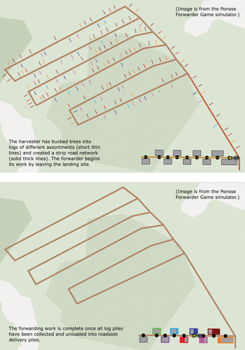
The FRP is defined here as follows. The harvester fells and bucks the trees into piles, each composed of a single assortment. The forwarder moves at constant speed along the strip roads. Due to its fixed carrying capacity, to complete the work, the forwarder must perform a series of tours. A tour starts with the forwarder at the roadside, then proceeds with the forwarder picking up piles until its capacity is full, after which the machine returns to the roadside and unloads the logs into delivery piles. Once the forwarder has unloaded the logs into delivery piles, the tour ends. Each tour is an ordered list of piles that the forwarder loads in succession. The route of the forwarder is the full, ordered list of piles required to complete the work. The forwarder always stops for loading and unloading. The work terminates when all logs from the harvesting site have been collected into delivery piles (Figure 1).

Figure 1. Schematic description of forwarding work at a CTL harvesting site.

The optimization goal is to minimize total distance traveled (D(r)), total time used (T(r)), and soil damage created (S(r)) with respect to the route r. As the time required for loading and unloading increases with the number of assortments (Manner et al. 2013; Figure 2), which generally happens with decreasing route length, and avoiding areas of a site susceptible to soil damage generally increases route length, the three objectives are conflicting. Thus, this FRP constitutes a multi-objective optimization problem (Jozefowiez et al. 2008) in which the vector-valued objective function (Eq. 1(1) $\left(D\left(r\right),T\left(r\right),S\left(r\right)\right)$(1) )

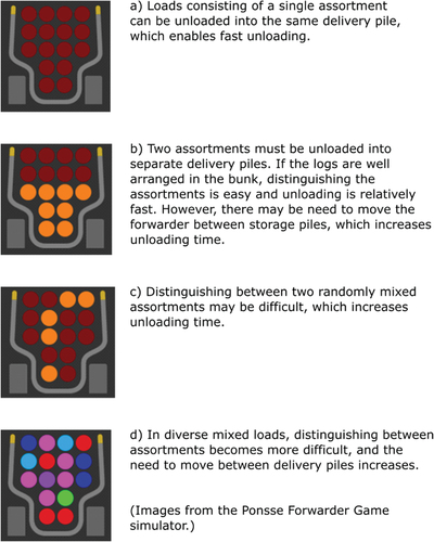
Figure 2. Illustration of the effect of the number of assortments on forwarder unloading time.

(1) $\left(D\left(r\right),T\left(r\right),S\left(r\right)\right)$(1)

is to be minimized. The FRP is treated here as a reverse vehicle routing problem (VRP; Toth and Vigo 2002; Jozefowiez et al. 2008) – instead of delivering resources from a depot to nodes that constitute a network, resources are gathered from the network to the depot.

Estimating the network of strip roads and piles

The FRP was modeled on a graph of log piles and strip roads deduced from real StanForD 2010 harvester data (HPR files; Skogforsk 2022). The network was composed of loading nodes, edges between these, and an unloading node. Each loading node corresponded to a unique log pile of a single assortment. The edges between loading nodes depicted strip roads along which the forwarder could move. The unloading node represented the delivery piles.

The HPR data does not directly contain data on created piles. Instead, for each processed stem, the volumes and assortments of created logs are recorded, paired with the GNSS location of the machine cabin when felling the stem. Therefore, the volumes and locations of piles needed to be estimated.

First, all produced logs labeled by their assortment were placed onto the easting-northing plane. Then, the positions and sizes of piles were estimated using a clustering algorithm (Figure 3).

Figure 3. The algorithm used for estimating the sizes and positions of assortment-specific log piles created by the harvester. The function “add neighbors” is separately expanded on the right.

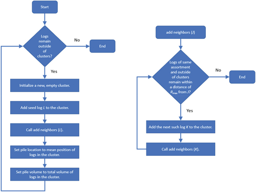
The clustering algorithm can be tuned through the parameter R_max (see Figure 3). Based on the available harvester data, R_max = 1.5 m produced piles of reasonable size in terms of number of logs in a pile, pile volume, and largest log-to-log distance in a pile (extent of pile). Piles smaller than 0.010 m³ in volume were discarded. These never constituted more than 1% of the piles at a harvest site.

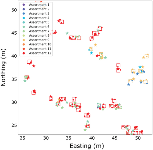
The logs processed by the harvester are assigned the position of the base machine. To diminish the possibility of placing two piles of different assortments on top of each other, a uniformly random displacement of −1.0 to 1.0 m in each coordinate dimension was added to every pile position. An example of the clustering is illustrated in Figure 4.

Figure 4. Example of estimating pile positions from harvester data. Squares represent the recorded position of the harvester cabin when felling a stem. This position is recorded for all logs from that stem. Dots depict the positions of the logs, to which small random noise has been added for purely visual purposes in this image. Stars depict the final, estimated pile positions.

The harvester data originated from four harvesting sites in South Finland. One spatially isolated, distinct area (system) of piles was cropped from each site for further processing. The properties of these systems are summarized in Table 1. As seen in Table 1, the clustering method occasionally created piles unrealistically large for typical Nordic cut-to-length harvesting operations (several m³ in volume, several m in spatial extent). However, they represented a minority, and the mean pile properties were reasonable.

Table 1. Summary of the harvester data used in this work. The area of each system and the removal per hectare are estimates. The system used for producing the route optimization results presented in the Results section is highlighted with italics. DBH stands for diameter at breast height, std for standard deviation.

System	Type of harvest	Number of piles	Number of logs in a pile	Volume of piles (m^3)	Pile extent (m)	Mean DBH (mm)	Species distribution	Total volume of harvested timber (m^3)	Area (ha)	Harvested timber per hectare (m^3/ha)	Total number of assortments
1	Thinning	448	1 to 33, mean 4.6, std 5.1	0.010 to 2.0, mean 0.27, std 0.30	0.00 to 7.3, mean 0.53, std 1.0	144	79.7% pine, 18.7% birch, 1.6% spruce	121	1.18	103	8
2	Clearcut	821	1 to 29, mean 3.1, std 2.9	0.013 to 7.3, mean 0.65, std 0.78	0.00 to 5.7, mean 0.34, std 0.74	282	95.5% spruce, 3.1% birch, 1.3% pine	537	1.97	273	9
3	Clearcut	2410	1 to 36, mean 2.8, std 2.6	0.011 to 2.0, mean 0.20, std 0.19	0.00 to 7.1, mean 0.31, std 0.70	155	45.0% spruce, 38.5% birch, 16.5% pine	487	5.16	94	13
4	Clearcut	1863	1 to 61, mean 3.2, std 4.3	0.012 to 3.3, mean 0.28, std 0.27	0.00 to 9.3, mean 0.45, std 0.95	179	92.8% pine, 5.7% spruce, 1.5% birch	516	4.30	120	10

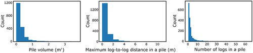
All systems described in Table 1 were used to develop and optimize the data pre-processing steps, in which logs were clustered into piles and the piles connected into networks. For the route optimization stage, systems 1, 2, and 3 were used to tune the parameters of the optimization algorithm. Finally, the optimization method was applied to system 4 (test system). Statistics on the created piles for system 4 are visualized in Figure 5.

Figure 5. Statistics on the created piles for system 4 (see Table 1).

The network of strip roads was estimated from the harvester GNSS data. As the GNSS measurements contain noise, they were smoothed using a sliding window of 7 m x 7 m over the position data. Within each window, the average position of points was computed and deduced to belong to a strip road at that position (road point).

Next, each pile was projected onto the trail. The projected locations of the piles described the locations where the forwarder was to stop for loading. For a given pile, the closest trail point (primary road point) was determined. Then, the three closest road points to the primary road point (secondary road points) were found, and a natural cubic spline was fitted through the primary and secondary road points. Finally, the pile was moved to the closest point P to it on the spline. For the studied systems 1–4, this projection procedure shifted the pile positions on average by 1.03 m, 1.17 m, 1.11 m, and 1.02 m, with a standard deviation of 0.833 m, 0.971 m, 0.883 m, and 0.819 m, respectively. Occasionally, two piles i and j ended up at the same position, in which case a distance of 0.5 m was assigned to the distance matrix element $D_{ij}$ in order to avoid numerical problems in the optimization. Over all studied systems and subproblems (see below), the mean fraction of distance matrix elements that were corrected in this way was too low (0.07% with a standard deviation of 0.1%) to be considered significant to the actual routing.

Having projected the piles onto the estimated strip road, the next step was to connect the piles to one another to form a network. The edges between piles, i.e., segments of strip roads between them, were created as follows. For a given pile i, the nearest pile j within a maximum distance D_max was found, and pile i was connected to j via the edge ij. Thereafter, an attempt to find the second-nearest neighbor k was made, requiring that k lie within a sector of angle α₀ on the opposite side of i and within a distance of D_max from i. If no such neighbor was found, the sector angle was increased by an amount Δα and the search repeated, until the sector spanned 360°. If k was found through this procedure, the edge ik was added. Finally, the length of each edge was set to the Euclidean distance between the two nodes. Tests on all four systems using D_max = 5, 10, …, 50 m; α₀ = 35, 40, …, 90°; Δα = 5, 10, 20, 30, 45, 90° showed that D_max = 30 m, α₀ = 65°, and Δα = 45° produced graphs that looked reasonably realistic. A single unloading node was then created by setting its location to the point on the nearest real-world forest road (deduced using a map) closest to the first felled stem. The real-life graph resulting from this procedure is illustrated in Figure 6(a) for system 4. It describes, within limits of approximation, the real network of piles and strip roads at the harvest site.

Figure 6. (a) The real-life graph created from a set of loading nodes and an estimate of the roadside delivery node location (gray dot) for system 4 (see Table 1) (b) Decomposition of the real-life graph into a disjoint set of region graphs.

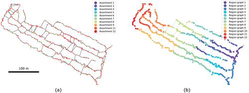
The aim here was not to strictly solve the FRP optimally for the full harvest area, because in practice, the forwarder typically works only on a region of the site at a time, starting out some time after the harvester. It is therefore more appropriate to optimize the forwarding work for a single region at a time. To reflect this, the real-life graph was decomposed into a set of disjoint region graphs for solving the total FRP as a set of independent subproblems. This decomposition operation is described in Figures 7 and 8.

Figure 7. The first part of the algorithm for decomposing the real-life graph into a set of disjoint region graphs. In this part of the algorithm, the set of subgraphs, which will be used to create the decomposition in the second part of the algorithm, is formed and then ordered by increasing distance from the unloading node.

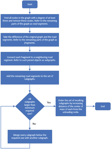
Figure 8. The second part of the algorithm for decomposing the real-life graph into a set of disjoint region graphs. In this part of the algorithm, the actual decomposition is constructed from the subgraphs created and ordered in the first part of the algorithm.

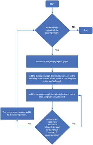
To keep solution times moderate, the mean number of nodes in a region graph was constrained to lie between 125 and 175. Tests performed on all four systems with the maximum allowed number of nodes in a region graph (see Figure 8) N^{max, nodes}_{region graph} = 50, 75, …, 300, and the minimum required number of nodes in a subgraph (see Figure 7) N^{min, nodes}_subgraph = 10, 15, 20, 30, 40, 50, 60, 70, 80, 90, 100 indicated that N^{max, nodes}_{region graph} = 125 and N^{min, nodes}_subgraph = 30 generally produced reasonable decompositions (Figure 6(b)). Finally, each resulting region graph was turned into a fully connected graph for solving the FRP independently for that region of the harvest site.

Modeling

A single tour of the forwarder consisted of picking up piles from a set of loading nodes and finally delivering these to the unloading node. More precisely, the ith tour was equal to the ordered list of nodes (0, n₁ⁱ, n₂ⁱ, …, 0) that the vehicle visits, beginning and ending with the unloading node (denoted by 0). The route that the forwarder takes to fully complete the work was the concatenated sum of these tours (0, n₁ⁱ⁼¹, n₂ⁱ⁼¹, …, 0, n₁ⁱ⁼², n₂ⁱ⁼², …, 0, …, 0). Visiting a loading node meant loading the entire pile at that node. A loading node was characterized by the assortment and total volume of logs that it holds. The roadside landing was described by an unloading node with no characteristics beyond those of a time consumption model for unloading.

For computing the real-life distance along strip roads between nodes i and j in the fully connected region graph, the shortest path between i and j in the connected real-life graph was found using Dijkstra’s algorithm (Dijkstra 1959; Hagberg et al. 2008) and tabulated into the matrix $D_{ij}$. Over all studied systems, the mean nearest-neighbor distance between loading nodes in a region graph ranged from 0.44 to 1.1 m. For computing the travel time $T_{ij}$ between any two nodes, the traversed distance was simply divided by the constant speed (Nurminen et al. 2006) of the forwarder (1 m/s).

Ground damage created when traversing the (shortest) path between nodes i and j was quantified as (Eq. 2(2) $S_{ij}=G_{ij}\left(1+\frac{V_{load}}{V_0}\right)=H_{ij}{D}_{ij}\left(1+\frac{V_{load}}{V_0}\right)$(2) ):

(2) $S_{ij}=G_{ij}\left(1+\frac{V_{load}}{V_0}\right)=H_{ij}{D}_{ij}\left(1+\frac{V_{load}}{V_0}\right)$(2)

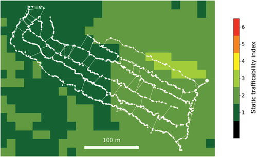
Here $G_{ij}=H_{ij}{D}_{ij}$, where $H_{ij}$ is the mean harvestability, i.e., mean trafficability along the path of length $D_{ij}$ along the strip roads, computed as the mean of the static trafficability index (Finnish Forest Centre 2020; Figure 9) under the nodes of the path. This index, provided on a grid of 16 m x 16 m cells throughout Finland, is an ordinal-scale six-class trafficability classification system from 1 (best bearing capacity, accessible even during spring thaw) to 6 (lowest bearing capacity, accessible only during the coldest periods of winter). The trafficability classes are predicted using soil type (mineral soil or peatland), average ground water height, the Topographic Wetness Index (TWI), and estimates of vegetation based on tree height distributions provided by the Finnish national laser scanning inventories (Bergqvist et al. 2018). While the static trafficability index is not a quantitative measure of the susceptibility of the ground to damage, it was treated as such here to quantify soil damage. Correspondingly, the created damage was interpreted as an index, not an empirically measurable quantity.

Figure 9. The static trafficability index for system 4 (see Table 1). The trafficability index is open data distributed by the Finnish Forest Centre (2020)

In Eq. 2(2) $S_{ij}=G_{ij}\left(1+\frac{V_{load}}{V_0}\right)=H_{ij}{D}_{ij}\left(1+\frac{V_{load}}{V_0}\right)$(2) , the term $\left(1+\frac{V_{load}}{V_0}\right)$ describes the effect of forwarder mass through the current load volume $V_{load}$ and the constant scaling factor $V_0$, the latter set here to 10 m³. The purpose of this term was to allow the damage to increase linearly with the load volume. One way of viewing the model is that $H_{ij}\left(1+\frac{V_{load}}{V_0}\right)$ describes the damage created by the machine per one meter of traveling between nodes i and j. The weaker the ground trafficability, and the greater the forwarder load, the more severe the rate of damage. The total damage from moving from i to j, for each pass, was then quantified by the product of damage per distance and traveled distance (Eq. 2)(2) $S_{ij}=G_{ij}\left(1+\frac{V_{load}}{V_0}\right)=H_{ij}{D}_{ij}\left(1+\frac{V_{load}}{V_0}\right)$(2) . The effect of multiple passes is not considered here.

Time consumed in loading (Eq. 3)(3) $t_{load}\left(n\right)=0.008336n^2+0.06435n+0.8678$(3) and unloading (Eq. 4)(4) $t_{unload}\left(n\right)=0.00792n^2+0.2312n+0.0909$(4) was modeled using the results of Manner et al. (2013):

(3) $t_{load}\left(n\right)=0.008336n^2+0.06435n+0.8678$(3)

(4) $t_{unload}\left(n\right)=0.00792n^2+0.2312n+0.0909$(4)

where time is in productive, delay-free machine minutes (treated here as regular time) per processed m³ of logs, and $n$ denotes the number of assortments in the load. Through these models, the time of loading or unloading was computed for a single, full load at a time. In the experimental setup behind these models, the configuration of delivery piles corresponded to average conditions.

Scalarization of the multi-objective optimization problem

For solving the FRP, the full harvest site was first decomposed into disjoint regions. Then, for each region, the multi-objective optimization problem of minimizing $\left(D\left(r\right),T\left(r\right),S\left(r\right)\right)$ (Eq. 1)(1) $\left(D\left(r\right),T\left(r\right),S\left(r\right)\right)$(1) was solved. To this end, a linear scalarization (Bowerman et al. 1995) of the multi-objective problem was first formulated using the cost function (Eq. 5(5) $c^{\prime }\left(r\right)=w_{distance}D\left(r\right)+w_{time}T\left(r\right)+w_{damage}S\left(r\right)$(5) ):

(5) $c^{\prime }\left(r\right)=w_{distance}D\left(r\right)+w_{time}T\left(r\right)+w_{damage}S\left(r\right)$(5)

where the scalars $w_{distance}$, $w_{time}$, and $w_{damage}$ are the weights given in the optimization to distance, duration, and soil damage, respectively. Through choosing values for the weights, the user can decide the importance of each objective in the optimization. $D\left(r\right)$ gives total distance traveled by the forwarder, i.e., the sum of $D_{ij}$ along the route. $T\left(r\right)=T_{load}\left(r\right)+T_{unload}\left(r\right)+T_{travel}\left(r\right)$ gives total time used for loading, unloading, and traveling, respectively. $T_{travel}\left(r\right)$ is equal to the sum of $T_{ij}$ along the route. $S\left(r\right)$ gives the total amount of ground damage created, i.e., the sum of $S_{ij}$ along the route.

The path connecting any two nodes in the region graph was fixed to the shortest path between these in the real-life graph, which placed a constraint on minimizing ground damage. However, the optimization algorithm was free to vary the order of visiting nodes, which should make it possible to avoid areas of poor trafficability to some degree, and furthermore to decrease total ground damage by considering load volume or by choosing a shorter route.

The routes that minimize $c^{\prime }\left(r\right)$ (Eq. 5)(5) $c^{\prime }\left(r\right)=w_{distance}D\left(r\right)+w_{time}T\left(r\right)+w_{damage}S\left(r\right)$(5) are Pareto optimal solutions to the original multi-objective problem. However, using Eq. 5(5) $c^{\prime }\left(r\right)=w_{distance}D\left(r\right)+w_{time}T\left(r\right)+w_{damage}S\left(r\right)$(5) directly in the optimization is problematic, as the different objective components inherently have different units and scales of magnitude (Bowerman et al. 1995). Therefore, components are normalized using their estimated average values in the region graph to arrive at the following cost function (Eq. 6)(6) $c\left(r\right)=w_{distance}\frac{D\left(r\right)}{\bar{D}}+w_{time}\frac{T\left(r\right)}{\bar{T}}+w_{damage}\frac{S\left(r\right)}{\bar{S}}$(6) :

(6) $c\left(r\right)=w_{distance}\frac{D\left(r\right)}{\bar{D}}+w_{time}\frac{T\left(r\right)}{\bar{T}}+w_{damage}\frac{S\left(r\right)}{\bar{S}}$(6)

Here $\bar{D}$, $\bar{T}$, and $\bar{S}$ are estimates for total distance, total duration, and total damage, respectively, for an “average” route. For total distance, the estimate was computed as (Eq. 7(7) $\bar{D}=2⟨D_{nn}⟩N_{nodes}^{subproblem}+\frac{4⟨D_{rsn}⟩V_{piles}^{subproblem}}{V_{capacity}^{forwarder}}$(7) ):

(7) $\bar{D}=2⟨D_{nn}⟩N_{nodes}^{subproblem}+\frac{4⟨D_{rsn}⟩V_{piles}^{subproblem}}{V_{capacity}^{forwarder}}$(7)

where $D_{nn}$ is the mean nearest-neighbor distance of piles in the region graph, $N_{nodes}^{subproblem}$ is the number of nodes in the region graph, $D_{rsn}$ is the direct distance from the unloading node to the mean position of piles in the region graph, $V_{piles}^{subproblem}$ is the total volume of piles in the region graph, and $V_{capacity}^{forwarder}$ is the forwarder loading capacity. For total duration, the estimate was computed as (Eq. 8(8) $\bar{T}=\frac{\bar{D}}{v_{forwarder}}+\left(t_{load}\left(n_{typical}\right)+t_{unload}\left(n_{typical}\right)\right)V_{piles}^{subproblem}$(8) ):

(8) $\bar{T}=\frac{\bar{D}}{v_{forwarder}}+\left(t_{load}\left(n_{typical}\right)+t_{unload}\left(n_{typical}\right)\right)V_{piles}^{subproblem}$(8)

where $v_{forwarder}$ is the speed of the forwarder and $n_{typical}$ is an estimate for a typical amount of assortments in a load, equal to $\mathrm{m}\mathrm{i}\mathrm{n}\left\{6,n_{subproblem}\right\}$, where $n_{subproblem}$ is the total number of different assortments in the region graph. For total damage, the estimate was computed as (Eq. 9(9) $\bar{S}=\left(2⟨H⟩⟨D_{nn}⟩N_{nodes}^{subproblem}+4⟨H⟩⟨D_{rsn}⟩V_{piles}^{subproblem}/V_{capacity}^{forwarder}\right)\left(1+\frac{V_{capacity}^{forwarder}/2}{V_0}\right)$(9) ):

(9) $\bar{S}=\left(2⟨H⟩⟨D_{nn}⟩N_{nodes}^{subproblem}+4⟨H⟩⟨D_{rsn}⟩V_{piles}^{subproblem}/V_{capacity}^{forwarder}\right)\left(1+\frac{V_{capacity}^{forwarder}/2}{V_0}\right)$(9)

where $⟨H⟩$ is the mean harvestability under the nodes of the region graph. The normalization in Eq. 6(6) $c\left(r\right)=w_{distance}\frac{D\left(r\right)}{\bar{D}}+w_{time}\frac{T\left(r\right)}{\bar{T}}+w_{damage}\frac{S\left(r\right)}{\bar{S}}$(6) cast the three objective components to dimensionless quantities each roughly of value 1, which made setting the importance of each component straightforward in the optimization.

The optimization algorithm

Due to the large number of piles, the FRP was solved using heuristic optimization. Ant Colony Optimization (ACO; Dorigo and Gambardella 1997; Bonabeau et al. 2000) was chosen as the underlying framework due to its flexibility and documented success in solving the VRP (Bullnheimer et al. 1999; Reimann et al. 2004). N_ants ants were first placed on the graph, each on a randomly chosen loading node. Then, in succession, one by one the ants independently completed a route through the graph, using as many tours as was necessary, visiting each loading node exactly once. A candidate list ${\mathrm{\Omega }}_i$, i.e., a list of the N_candidates nearest loading nodes for each node i, was employed. During the construction of a route, an ant located at node i moved to node j according to the following transition rule. Provided that unvisited nodes still remained in the candidate list of node i, the ant moved to node j with probability (Eq. 10(10) $p_{ij}=\left\{\begin{array}{c}\frac{{\tau }_{ij}^{\alpha }{\eta }_{ij}^{\beta }}{\sum {\tau }_{ij}^{\alpha }{\eta }_{ij}^{\beta }},j\in {\mathrm{\Omega }}_i\\ 0,otherwise\end{array}\right.$(10) ):

(10) $p_{ij}=\left\{\begin{array}{c}\frac{{\tau }_{ij}^{\alpha }{\eta }_{ij}^{\beta }}{\sum {\tau }_{ij}^{\alpha }{\eta }_{ij}^{\beta }},j\in {\mathrm{\Omega }}_i\\ 0,otherwise\end{array}\right.$(10)

where ${\eta }_{ij}$ is the heuristic desirability of node j as seen from node i, and ${\tau }_{ij}$ is the (asymmetrical) amount of virtual pheromone along the edge ij. If no unvisited nodes remained in the candidate list, the ant moved to the node of highest heuristic desirability. The desirability was computed as (Eq. 11(11) ${\eta }_{ij}=\frac{1}{w_{distance}\frac{D_{ij}}{\bar{d}}+w_{time}\frac{T_{ij}}{\bar{t}}+w_{damage}\frac{S_{ij}}{\bar{s}}}$(11) ):

(11) ${\eta }_{ij}=\frac{1}{w_{distance}\frac{D_{ij}}{\bar{d}}+w_{time}\frac{T_{ij}}{\bar{t}}+w_{damage}\frac{S_{ij}}{\bar{s}}}$(11)

Here $\bar{d}$, $\bar{t}$, and $\bar{s}$ are estimates of the average value of the distance between two nodes, the time of traversing an edge, and the damage created when traversing an edge, respectively. For distance, the estimate was computed as (Eq. 12(12) $\bar{d}=\frac{⟨D_{ij}⟩}{2}$(12) ):

(12) $\bar{d}=\frac{⟨D_{ij}⟩}{2}$(12)

where $D_{ij}$ is the mean of the distance matrix elements for the region graph. For time, the estimate was computed as (Eq. 13(13) $\bar{t}=\frac{\bar{d}}{v_{forwarder}}$(13) ):

(13) $\bar{t}=\frac{\bar{d}}{v_{forwarder}}$(13)

For soil damage, the estimate was computed as (Eq. 14(14) $\bar{s}=\bar{d}⟨H⟩\left(1+\frac{V_{capacity}^{forwarder}/2}{V_0}\right)$(14) ):

(14) $\bar{s}=\bar{d}⟨H⟩\left(1+\frac{V_{capacity}^{forwarder}/2}{V_0}\right)$(14)

The normalization constants cast each of the three components in the denominator of ${\eta }_{ij}$ to dimensionless quantities roughly of value 1.

After each transition from node i to j, the pheromone concentration on the edge ij was updated via (Eq. 15(15) ${\tau }_{ij}=\left(1-\rho \right){\tau }_{ij}+\rho {\tau }_0$(15) ):

(15) ${\tau }_{ij}=\left(1-\rho \right){\tau }_{ij}+\rho {\tau }_0$(15)

where $\rho$ is a parameter governing the rate of pheromone decay, and ${\tau }_0$ is the value that the pheromone concentration on all edges was originally initialized to (here 1/(N_nodesC_typical), where N_nodes is the number of nodes and C_typical is the cost of an “average” quality solution). After all ants had completed a route, one iteration of the algorithm was complete. Then, pheromone values were updated on all edges belonging to the route of the lowest cost $C^{\ast }$ so far via (Eq. 16(16) ${\tau }_{ij}=\left(1-\rho \right){\tau }_{ij}+\frac{\rho }{C^{\ast }}$(16) ):

(16) ${\tau }_{ij}=\left(1-\rho \right){\tau }_{ij}+\frac{\rho }{C^{\ast }}$(16)

As the iterations continued, one kept track of the route of lowest cost, this constituting the iteratively improving solution to the FRP. The purpose of the desirability (Eq. 11)(11) ${\eta }_{ij}=\frac{1}{w_{distance}\frac{D_{ij}}{\bar{d}}+w_{time}\frac{T_{ij}}{\bar{t}}+w_{damage}\frac{S_{ij}}{\bar{s}}}$(11) was to guide the search for solutions according to the objective weights in the cost function (Eq. 6)(6) $c\left(r\right)=w_{distance}\frac{D\left(r\right)}{\bar{D}}+w_{time}\frac{T\left(r\right)}{\bar{T}}+w_{damage}\frac{S\left(r\right)}{\bar{S}}$(6) . Pheromone replenishment (Eq. 16(16) ${\tau }_{ij}=\left(1-\rho \right){\tau }_{ij}+\frac{\rho }{C^{\ast }}$(16) ) was controlled by the cost of the best route found so far, which similarly directed the search according to the objective weights.

The desirability ${\eta }_{ij}$ can be viewed as a measure of how good the transition from i to j appears to the ant from a local viewpoint. The pheromone ${\tau }_{ij}$ along the edges represents how good the transition from i to j has generally proven as part of a route. The constants $\alpha$ and $\beta$ can be used to tune the relative contribution of desirability and pheromone in the transition probabilities.

The optimization algorithm code was written in Python 3 and is freely available at https://github.com/ekholmst/smartlog_aco.

Computations

A set of optimizations was first performed on an artificial system of ten piles and two assortments. This was done to verify the intuitively correct behavior of the algorithm for each objective component. The pile volumes, forwarder capacity, and forwarder speed were chosen for each case of the objective component so that the optimal solution would be clear beforehand, and that the correct functioning of the optimization algorithm would therefore be easily verifiable. Then, multi-objective optimization was done for distance and duration using an artificial system of 50 piles and five assortments, to verify the expected trade-off between the two objectives. 500 iterations, a constant harvestability of 1, and $\rho =0.01$ was used in these runs. The parameters $\alpha$ and $\beta$ were separately optimized for each case.

Next, to find generally well-performing values for $\alpha$, $\beta$, and $\rho$ for real harvest sites, a grid search was performed with $\alpha$ = 0, 1, …, 6; $\beta$ = 0, 1, …, 6; $\rho$ = 0.01, 0.05, 0.10, 0.25, 0.50, 0.75 on systems 1, 2, and 3. A total of 50 iterations were run using five random initializations for each set of parameter values for each system, optimizing separately for distance, duration, and damage. These results were analyzed to find fixed values for $\alpha$, $\beta$, and $\rho$ that should produce good results over different systems and choices of objective metrics.

Finally, using the optimized values of $\alpha$, $\beta$, and $\rho$, the full optimization strategy was applied to the test system. Optimization was first done separately each objective. For reference, the equivalent runs were also performed using a uniformly random search ($\alpha =\beta =0$). Then, multi-objective optimization was performed for pairs of objective metrics. The results were averaged over 10 random initializations in single-objective optimization and 50 initializations in multi-objective optimization. In these computations, 500 iterations were used.

In all runs throughout this work, N_ants was set to the number of loading nodes considered in the optimization, and N_candidates was set to 20.

Results

Optimization on small model systems

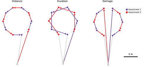
Results of single-objective optimization on the artificial model system are presented in Figure 10. The volume of each pile was 2 m³. For the case of distance minimization, forwarder capacity was set to 20 m³ and speed to 1 m/s. As expected, distance was minimized by picking up the piles in succession along the circular road. The optimal solution was always found with $\beta \ge 2$. In minimizing duration, to illustrate the effect of loading and unloading time, the forwarder speed was set to infinite and capacity to 10 m³. In the best solution, all piles of assortment 1 were picked up in the first tour and all piles of assortment 2 in the second tour. This optimal solution was found generally with $\beta =0$ and in some cases with $\beta =2$. For the case of damage minimization, the forwarder speed was set to 1 m/s and capacity to 10 m³. The algorithm correctly guided the forwarder to drive out empty and then to pick up piles as it approached the roadside node. This optimal solution was found generally with $\beta \ge 2$. The value of $\alpha$ was not significant in the optimizations of these simplistic systems.

Figure 10. Optimized routes on the artificial model system. The solutions illustrate how the optimization algorithm separately minimizes distance, duration, and damage. The color of the arrow indicates the assortment of the destination node at each step of the route.

The system used for verifying multi-objective optimization is presented in Figure 11. Each pile had a volume of 1 m³. Speed and capacity of the forwarder were set to 1 m/s and 10 m³, respectively. The weight values were $w_{distance}$ = 0.5, $w_{time}$= 0.5, and $w_{damage}$ = 0.0. The values $\alpha =4$, $\beta =2$ proved optimal here. For comparison, single-objective optimization runs for distance and duration were made. For the former, high $\beta$ was a good choice. For the latter, best results were obtained with a high $\alpha$ and low $\beta$.The results, presented in Table 2, show that multi-objective optimization produced a trade-off between distance and duration, as well as the number of assortments in the loads.

Figure 11. Artificial model system used to illustrate multi-objective optimization.

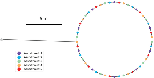
Table 2. Multi-objective optimization results for distance and duration on the artificial model system, and corresponding single-objective results for comparison.

Optimization criteria	Route length (m)	Duration (h)	Number of assortments in load
Distance	204.2	2.4	5
Distance and duration	230.5	1.9	3 to 4
Duration	275.6	1.5	2 to 3

Optimizing the ACO parameters for real harvest sites

In the parameter search on real harvest site data, it was found that generally, $\alpha =\beta =0$, i.e., a uniformly random search, gave the worst results. Making $\alpha$ nonzero generally improved the results, and making $\beta$ nonzero further improved the results. However, pheromone alone was not a strong driver in the search for solutions, and in many cases, the uniformly random search found better solutions than when using $\alpha =1,\beta =0$. Still, using any combination of $\alpha \ne 0,\beta \ne 0$, i.e., running the full optimization algorithm, gave significantly better results than a uniformly random search. In the grid search, the best parameter values provided an improvement of 5% to 10% in duration and 20% to 40% in distance or damage with respect to the random search.

These parameter optimization results showed that optimizing solely for distance or damage was done most efficiently with a large value of $\beta$ and a slightly smaller value of $\alpha$. In contrast, optimizing for duration was most efficient with a large value for $\alpha$ and a slightly smaller value for $\beta$. This is reasonable, as optimizing either distance or damage should benefit from emphasizing transitions between loading nodes close to one another, as dictated by $\beta$. Conversely, “learning” routes that minimize loading and unloading times, as is relevant in minimizing duration, is solely up to the pheromone, as dictated by $\alpha$. This reflects the findings on the small model systems presented in the previous subsection. Overall, a good compromise of parameter values was $\alpha$ = 5, $\beta$ = 4, $\rho$ = 0.01.

All essential parameter values used in producing the results of the next two subsections are presented in Table 3.

Table 3. Essential parameter values used in optimizing the test system.

Parameter	Value
Forwarder loading capacity	12 m^3
Forwarder speed	1 m/s
$V_0$ in the ground damage model	10 m^3
$\rho$	0.01
$\alpha$	5
$\beta$	4
Number of ants	Number of loading nodes in the region graph
Length of candidate list	20
Number of ACO iterations	500

Single-objective optimization on a real harvest site

The single-component optimization results for the test system are summarized in Table 4. As expected, the best value for each objective was found where that particular objective was being minimized. In Table 4, the mean number of unique assortments over the forwarder loads is also reported. On average, optimizing duration led to loads having a lower number of assortments, in comparison to the case of optimizing distance or damage. Loading and unloading consumed more time the more assortments were involved (Equations 3(3) $t_{load}\left(n\right)=0.008336n^2+0.06435n+0.8678$(3) and 4(4) $t_{unload}\left(n\right)=0.00792n^2+0.2312n+0.0909$(4) ). Therefore, for optimizing duration, it was beneficial to pick up fewer different assortments on a tour, although this implied longer routes. The reference runs performed using a uniformly random search ($\alpha =\beta =0$) showed that using the full ACO algorithm improved the results by 8–25% depending on the objective.

Table 4. Results for optimizing forwarder work in the test system using a single objective at a time. The best value for each metric is set in italics. Each result is an average over 10 randomly initialized optimizations. The error is the standard error of the mean.

Optimization criterion	Distance (km)	Duration (h)	Damage	Mean number of assortments in load
Distance	24.13 ± 0.07	30.28 ± 0.04	67,680 ± 120	4.63 ± 0.08
Duration	26.29 ± 0.07	28.48 ± 0.03	72,280 ± 140	4.16 ± 0.07
Damage	24.52 ± 0.07	30.54 ± 0.06	66,530 ± 100	4.67 ± 0.07

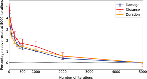
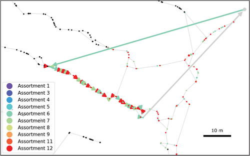
An example of optimized routes for a given region of the harvest area is shown in Figure 12. A more detailed example is provided in Figure 13 for each case of single-objective optimization. Regardless of the metric being optimized, the routes produced consisted largely of stretches of picking up piles in relatively straightforward succession along the roads. Such relatively smooth routing could be expected to be of practical value to human forwarder operators. However, in some parts of the graphs, the network creation algorithm produced structures of spurious appearance (Figures 6, 13b). Therefore, a smoothening or simplification of the graph structure would probably be necessary before practical applications. In addition, although producing metric values within 1–2% of the values obtained with very long runs (Figure 14), the 500 iterations used in these results was not enough for attaining completely converged routes. Together, these two effects most likely led to somewhat “noisy” routes.

Figure 12. Example of a general view of optimized routes for a given region of the harvest site when minimizing total traveled distance. The arrows denote the order in which piles are picked up, with the color of the arrow indicating the assortment of the destination pile at each step along the route. Each transition between nodes (e.g., from the unloading node to the first node to be visited, i.e., pile to be loaded) is done along the shortest path on the strip road network. The long arrows denote transitions between the unloading node and the loading nodes.

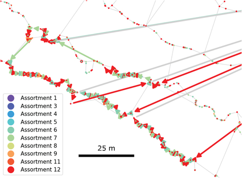
Figure 13. Close-up views of routes optimized considering only a single objective at a time: distance (a, b), duration (c), and soil damage (d). The arrows depict the route of the forwarder, with the color of the arrow indicating the assortment of the destination pile at each step of the route.

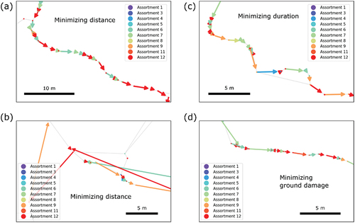
Figure 14. Convergence behavior of the optimization algorithm when optimizing one objective at a time. Each point is an average over 10 randomly initialized optimizations. The error is the standard error of the mean.

The formulation for modeling ground damage (Eq. 2)(2) $S_{ij}=G_{ij}\left(1+\frac{V_{load}}{V_0}\right)=H_{ij}{D}_{ij}\left(1+\frac{V_{load}}{V_0}\right)$(2) linked damage creation strongly with route length. Therefore, routes produced when optimizing only for distance or ground damage displayed similar length and damage (Table 4). However, in comparison to minimizing only distance, minimizing damage typically tended to route the forwarder so that as piles were being picked up, the machine approached the roadside landing (Figure 15). The total amount of ground damage decreased in this way, as the working pattern reduced the distance driven loaded.

Figure 15. When minimizing ground damage, the optimized routes often displayed working patterns where the forwarder picks up piles while approaching the landing. This is a way of decreasing the total soil damage created.

Multi-objective optimization on a real harvest site

In this work, the objective vector was scalarized linearly (Eq. 6)(6) $c\left(r\right)=w_{distance}\frac{D\left(r\right)}{\bar{D}}+w_{time}\frac{T\left(r\right)}{\bar{T}}+w_{damage}\frac{S\left(r\right)}{\bar{S}}$(6) using the weights $w_{distance}$, $w_{time}$, and $w_{damage}$, which dictate the relative importance of each objective in the optimization. Considering any two of the three objectives (distance, duration, damage) at a time, and by varying the weights of the objectives, trends reflecting these importance preferences were observed in the metrics (Figure 16). The routes themselves qualitatively resembled the single-objective optimized routes found in the previous subsection.

Figure 16. Results for optimizing two objective components at a time, using different values for the objective weights (Eq. 6)(6) $c\left(r\right)=w_{distance}\frac{D\left(r\right)}{\bar{D}}+w_{time}\frac{T\left(r\right)}{\bar{T}}+w_{damage}\frac{S\left(r\right)}{\bar{S}}$(6) . The weight (w) of the component plotted on the left vertical axis is given on the horizontal axis. The weight of the component plotted on the right vertical axis is equal to 1 – w. Each point is an average over 50 randomly initialized optimizations. The error is the standard error of the mean.

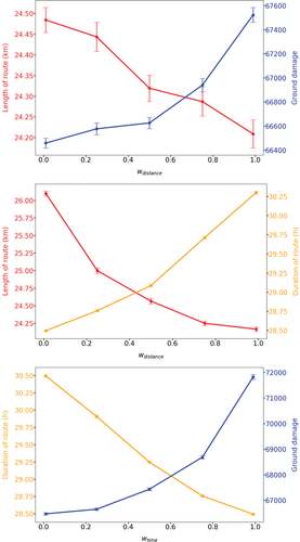
As noted above, the route length and ground damage were strongly linked in the present model, which did not allow for large variance in these objectives even though their respective weights were varied (Figure 16, top). However, for the objective pairs of route length and duration, as well as duration and ground damage, the effect of varying the weights was strong and clear (Figure 16, middle and bottom).

Discussion

In this paper, a strategy for optimizing forwarding work in CTL harvesting operations through multi-objective optimization of route length, duration, and created ground damage was presented. The strategy is modular, which enables one to easily change the models, including the time consumption model, and the currently simplistic model for ground damage creation. A smoothening of the graph structure is likely necessary for increasing the practical value of the approach. The clustering method for estimating piles can also be replaced. Topography of the terrain, affecting both the speed and fuel consumption of the forwarder, is an important aspect to be implemented in the future. Fuel consumption could also be included as a minimization objective.

In the cost function (Eq. 6(6) $c\left(r\right)=w_{distance}\frac{D\left(r\right)}{\bar{D}}+w_{time}\frac{T\left(r\right)}{\bar{T}}+w_{damage}\frac{S\left(r\right)}{\bar{S}}$(6) ), the normalization factor $\bar{S}$ was directly proportional to mean trafficability over the subproblem being optimized. It follows that the variation of the trafficability index H within a subproblem impacts the routing through placing more emphasis on damage minimization where H is high, generally creating shorter routes with more assortments per load in those areas. However, for constant H within a subproblem, the value of H cancels out and does not affect forwarder routing. An alternative approach would be to use the average of H over the full harvest site in computing $\bar{S}$. Also, for real forest operations, using a trafficability map updated dynamically to reflect weather conditions would be more useful than the currently demonstrated static one. For regions outside of Finland, a corresponding numerical matrix of trafficability values, where higher is worse, would need to be provided.

In the present approach, $\frac{T_{ij}}{\bar{t}}=\frac{D_{ij}}{\bar{d}}$ in Eq. 11(11) ${\eta }_{ij}=\frac{1}{w_{distance}\frac{D_{ij}}{\bar{d}}+w_{time}\frac{T_{ij}}{\bar{t}}+w_{damage}\frac{S_{ij}}{\bar{s}}}$(11) . Another approach, which would more strongly direct the search for smaller route duration, would be to introduce a dependency into $T_{ij}$ on the number of assortments in the load after loading pile j.

Accurate positioning of the harvester head could make data on pile assortment and location directly available (Lindroos et al. 2015; Müller et al. 2019). Some harvesters already record the estimated crane tip position upon felling the stem. In an intermediate scenario, the role of route optimization, for both human operators and autonomous forwarders, could be one of a supporting system, which guides the machine close to a recommended pick-up location, after which the operator or machine sensors observe the actual piles to be picked up.

With the current implementation, solving the FRP on the test system using 500 iterations takes approximately 30 min per harvest site region on a single CPU core. As good convergence was attained already at 200–300 iterations (Figure 14), the computing time could be reduced to approximately 15 min per region.

The framework of this study could also be harnessed to assess the productivity and cost of alternative working patterns given as input by the user. A broader set of harvest sites should be explored in order to gauge the applicability of the method beyond the sample data used in this study. Ultimately, the power and practical value of the presented optimization strategy should be assessed in experiments involving human operators.

Conclusions

In this work, a multi-objective optimization strategy for timber forwarding in cut-to-length harvesting operations was presented. The approach allows for simultaneous optimization of several conflicting objectives in finding the optimal route of the forwarder on a preexisting network of strip roads and log piles. The strategy consists of estimating pile positions and the strip road network from standard harvester data, modeling of forwarder movement, time consumption of work phases, and soil damage, and finally heuristically solving a linearized form of the multi-objective optimization problem on a fully connected network. The sensibility and effectiveness of the approach was shown in computational tests on artificial and real harvest site data. Field tests involving human operators should be carried out in the future to assess the usefulness of the method in real forest operations. The optimization code has been made publically available.

Acknowledgements

The authors thank H. Lindeman, A. Raatevaara, J. Ala-Ilomäki, and M. Sirén for advice and fruitful discussions. The authors gratefully acknowledge Metsähallitus and Metsäkonepalvelu Oy for providing the harvester data. The authors acknowledge CSC – IT Center for Science, Finland, for computational resources. EH thanks M. Holsti and M. Saari for enabling field observations of real forwarding operations.

Disclosure statement

No potential conflict of interest was reported by the authors.

Additional information

Funding

This work was supported by the SmartLog project (no. 41007-00119100) and SecureLog project (no. 41007-00211300) at Luke, the Academy of Finland Flagship “Forest-Human-Machine Interplay – Building Resilience, Redefining Value Networks and Enabling Meaningful Experiences” (funding decision 337655), and the Academy of Finland project “Trafficability Prediction and Route Planning for Forest Machines” (funding decision 332172).

References

- Ala-Ilomäki J, Salmivaara A, Launiainen S, Lindeman H, Kulju S, Finér L, Heikkonen J, Uusitalo J. 2020. Assessing extraction trail trafficability using harvester CAN-bus data. Int J For Eng. 2:138–145.
- Başkent EZ. 2018. A review of the development of the multiple use forest management planning concept. Int For Rev. 20(3):296–313. doi:10.1505/146554818824063023.
- Bergqvist I, Willén E, Peuhkurinen J, Väätäinen K, Lindeman H, Lauren A, Poikela A. 2018. EFFORTE Deliverable D3.3. – forest trafficability maps – data sources and methods. [accessed 2022 Feb 23]. http://www.luke.fi/efforte
- Björheden R, Thompson MA 1995. An international nomenclature for forest work study. In: Field DB, editor. Proceedings, IUFRO 1995; 6–12 Aug; Tampere, Finland. S3:04.
- Bonabeau E, Dorigo M, Theraulaz G. 2000. Inspiration for optimization from social insect behaviour. Nature. 406:39–42.
- Bowerman R, Hall B, Calamai P. 1995. A multi-objective optimization approach to urban school bus routing: formulation and solution method. Transport Res A-Pol. 29(2):107–123.
- Bullnheimer B, Hartl RF, Strauss C. 1999. An improved ant system algorithm for the vehicle routing problem. Ann Oper Res. 89:319–328. doi:10.1023/A:1018940026670.
- Chugunkova AV, Pyzhev A. 2020. Impacts of global climate change on duration of logging season in Siberian boreal forests. Forests. 11(7):756. doi:10.3390/f11070756.
- Dijkstra EW. 1959. A note on two problems in connexion with graphs. Numer Math. 1:269–271. doi:10.1007/BF01386390.
- Dorigo M, Gambardella LM. 1997. Ant colony system: a cooperative learning approach to the traveling salesman problem. IEEE T Evolut Comput. 1(1):53–66. doi:10.1109/4235.585892.
- Eriksson M, Lindroos O. 2014. Productivity of harvesters and forwarders in CTL operations in northern Sweden based on large follow-up datasets. Int J For Eng. 25(3):179–200.
- FAO. 2020. Global forest resources assessment 2020: main report. Rome.
- Finnish Forest Centre. 2020. Harvestability maps of Finland. [accessed 2020 Nov 20]. https://www.metsakeskus.fi/korjuukelpoisuuskartat.
- Flisberg P, Forsberg M, Rönnqvist M. 2007. Optimization based planning tools for routing of forwarders at harvest areas. Can J Forest Res. 37(11):2153–2163. doi:10.1139/X07-065.
- Flisberg P, Rönnqvist M, Willén E, Frisk M, Friberg G. 2021. Spatial optimization of ground-based primary extraction routes using the BestWay decision support system. Can J Forest Res. 51(5):675–691. doi:10.1139/cjfr-2020-0238.
- Friberg G 2014. En analysmetod för att optimera skotning mot minimerad körsträcka och minimerad påverkan på mark och vatten [A method to optimize forwarding towards minimized driving distance and minimized effect on soil and water] [master’s thesis]. Uppsala (Sweden): SLU. https://stud.epsilon.slu.se/6956/1/Friberg_G_20140630.pdf.
- Hagberg AA, Schult DA, Swart PJ 2008. Exploring network structure, dynamics, and function using NetworkX. In: Varoquaux G, Vaught T, Millman J, editors. Proc Pyth Sci Conf (SciPy2008); Pasadena (CA), USA. p. 11–15.
- Han H-S, Page-Dumroese DS, Han SK, Tirocke J. 2006. Effects of slash, machine passes, and soil moisture on penetration resistance in a cut-to-length harvesting. Int J For Eng. 17(2):11–24.
- Hoffmann S, Schönauer M, Heppelmann J, Asikainen A, Cacot E, Eberhard B, Hasenauer H, Ivanovs J, Jaeger D, Lazdins A, et al. 2022. Trafficability prediction using depth-to-water maps: the status of application in northern and Central European forestry. Curr For Rep. 2022:1–17.
- Holm S, Frutig F, Lemm R, Thees O, Schweier J. 2020. HePrMo: a decision support tool to estimate wood harvesting productivities. PLOS ONE. 15(12):e0244289. doi:10.1371/journal.pone.0244289.
- Hoogstra-Klein MA, Brukas V, Wallin I. 2017. Multiple-use forestry as a boundary object: from a shared ideal to multiple realities. Land Use Policy. 69:247–258. doi:10.1016/j.landusepol.2017.08.029.
- Iasevoli G, Massi M. 2012. The relationship between sustainable business management and competitiveness: research trends and challenge. Int J Technol Manage. 58(1–2):32–49. doi:10.1504/IJTM.2012.045787.
- John Deere: TimberMatic Maps. [accessed 2022 Feb 23]. https://www.deere.co.uk/en/forestry/timbermatic-manager/
- Jozefowiez N, Semet F, Talbi E-G. 2008. Multi-objective vehicle routing problems. Eur J Oper Res. 189(2):293–309. doi:10.1016/j.ejor.2007.05.055.
- Jylhä P, Jounela P, Koistinen M, Korpunen H. 2019. Koneellinen hakkuu. Seurantatutkimus. [Mechanised cutting. Follow-up study]. Helsinki: Natural Resources Institute Finland (Luke). Nov.
- Komatsu Forest: MaxiVision. [accessed 2022 Feb 23]. https://www.komatsuforest.com/services/maxivision.
- Koŝir B, Magagnotti N, Spinelli R. 2015. The role of work studies in forest engineering: status and perspectives. Int J For Eng. 26(3):160–170.
- Lehtonen I, Venäläinen A, Kämäräinen M, Asikainen A, Laitila J, Anttila P, Peltola H. 2019. Projected decrease in wintertime bearing capacity on different forest and soil types in Finland under a warming climate. Hydrol Earth Syst Sci. 23:1611–1631. doi:10.5194/hess-23-1611-2019.
- Lindroos O, Ringdahl O, Hera P, Hohnloser P, Hellström T. 2015. Estimating the position of the harvester head – a key step towards the precision forestry of the future? Croat J For Eng. 36. 2:147–164.
- Manner J 2015. Automatic and experimental methods to studying forwarding work [dissertation]. Umeå (Sweden): SLU.
- Manner J, Nordfjell T, Lindroos O. 2013. Effects of the number of assortments and log concentration on time consumption for forwarding. Silva Fenn. 47(4):1–19. doi:10.14214/sf.1030.
- Marchi E, Chung W, Visser R, Abbas D, Nordfjell T, Mederski PS, McEwan A, Brink M, Laschi A. 2018. Sustainable Forest Operations (SFO): a new paradigm in a changing world and climate. Sci Total Environ. 634:1385–1397. doi:10.1016/j.scitotenv.2018.04.084.
- Müller F, Jaeger D, Hanewinkel M. 2019. Digitization in wood supply – a review on how Industry 4.0 will change the forest value chain. Comp Elec Agric. 162:206–218. doi:10.1016/j.compag.2019.04.002.
- Nugent C, Kanali C, Owende PMO, Nieuwenhuis M, Ward S. 2003. Characteristic site disturbance due to harvesting and extraction machinery traffic on sensitive forest sites with peat soils. Forest Ecol Manag. 180(1–3):85–98. doi:10.1016/S0378-1127(02)00628-X.
- Nurminen T, Korpunen H, Uusitalo J. 2006. Time consumption analysis of the mechanized cut-to-length harvesting system. Silva Fenn. 40(2):335–363. doi:10.14214/sf.346.
- Palander T, Kärhä K. 2021. Utilization of image, LiDAR and gamma-ray information to improve environmental sustainability of cut-to-length wood harvesting operations in peatlands: a management systems perspective. ISPRS Int J Geo-Inf. 10(5):273. doi:10.3390/ijgi10050273.
- Picchio R, Latterini F, Mederski PS, Tocci D, Venanzi R, Stefanoni W, Pari L. 2020. Applications of GIS-based software to improve the sustainability of a forwarding operation in Central Italy. Sustainability. 12(14):5716. doi:10.3390/su12145716.
- Ponsse: Forwarder systems overview. [accessed 2022 Feb 23]. https://www.ponsse.com/en/web/guest/products/information-systems/product/-/p/forwarder_systems#/.
- Reimann M, Doerner K, Hartl RF. 2004. D-ants: savings based ants divide and conquer the vehicle routing problem. Comput Oper Res. 31(4):563–591. doi:10.1016/S0305-0548(03)00014-5.
- Ringdahl O, Lindroos O, Hellström T, Bergström D, Athanassiadis D, Nordfjell T. 2011. Path tracking in forest terrain by an autonomous forwarder. Scand J Forest Res. 26(4):350–359. doi:10.1080/02827581.2011.566889.
- Salmivaara A, Launiainen S, Perttunen J, Nevalainen P, Pohjankukka J, Ala-Ilomäki J, Sirén M, Laurén A, Tuominen S, Uusitalo J, et al. 2020. Towards dynamic forest trafficability prediction using open spatial data, hydrological modelling and sensor technology. Forestry. 93(5):662–674. doi:10.1093/forestry/cpaa010
- Salmivaara A, Miettinen M, Finér L, Launiainen S, Korpunen H, Tuominen S, Heikkonen J, Nevalainen P, Sirén M, Ala-Ilomäki J, et al. 2018. Wheel rut measurements by forest machine-mounted LiDAR sensors – accuracy and potential for operational applications? Int J For Eng. 29(1):41–52.
- Seppälä P 2020. Tavaralajimenetelmän metsäkoneiden automaation kehitysnäkökulmat [Prospects of automation development in cut-to-length harvesting forest machines]. Metsätehon raportti 259. http://www.metsateho.fi/wp-content/uploads/Raportti-259-Tavaralajimenetelman-metsakoneiden-automaation.pdf.
- Skogforsk. 2022. Stanford 2010. [accessed 2022 Feb 23]. https://www.skogforsk.se/english/projects/stanford/stanford-2010/.
- Toth P, Vigo D. 2002. Models, relaxations and exact approaches for the capacitated vehicle routing problem. Discrete Appl Math. 123(1–3):487–512. doi:10.1016/S0166-218X(01)00351-1.
- United Nations. 2019. United Nations Forum on Forests. Report on the fourteenth session (11 May 2018 and 6–10 May 2019). Economic and Social Council Official Records, Supplement No. 22. E/2019/42-E/CN.18/2019/9. New York.
- Väätäinen K, Lamminen S, Ala-Ilomäki J, Sirén M, Asikainen A. 2013. Kuljettajaa opastavat järjestelmät koneellisessa puunkorjuussa – kooste hankkeen avaintuloksista. Helsinki: Metla. Metlan työraportteja 279.
- Westlund K 2011. Optimerad skotning av rundvirke, grot och stubbar [Optimized forwarding of roundwood, logging residues, and stumps]. Uppsala (Sweden): Skogforsk. Resultat 18. https://www.skogforsk.se/cd_20190114161735/contentassets/7e126b5d70d7432293ee152c960361ec/resultat-nr-18-2011_low.pdf
- Ylimäki R, Väätäinen K, Lamminen S, Sirén M, Ala-Ilomäki J, Ovaskainen H, Asikainen A 2012. Kuljettajaa opastavien järjestelmien tarve ja hyötypotentiaali koneellisessa puunkorjuussa [The need and potential for benefit of operator-assisting systems in mechanized wood harvesting]. Helsinki: Metla. Metlan työraportteja 224. http://www.metla.fi/julkaisut/workingpapers/2012/mwp224.pdf