Rail transport in Swedish wood supply – seasonal variation, system risks and mitigation costs

ABSTRACT

This study examines the potential for reduced risks in roundwood transport by rail. The study quantifies seasonal variation and system risks under boreal conditions, as well as practical routines for managerial response to these. The study case is based on an integrated forest company with 11 supply terminals supplying coastal mills in mid-Sweden. The terminals were distributed from south to north Sweden, with six core terminals located in the interior- and mid-supply zones for coastal mills. The monthly flows ranged from 75 to 118% of the annual average and the monthly variability of terminal inflows was 67% higher for the interior than the mid-zone terminals. Comparing inflows between assortments, the lowest variability was for coniferous pulpwood (8%) and pine sawlogs (18%), increasing thereafter to deciduous pulpwood (28%) and spruce sawlogs (53%). Regarding rail system disturbances, the frequency of deviations from scheduled routes for the core terminals was 16–17%, resulting in canceled routes for 53–65% of deviations. Two mitigation scenarios were tested to reduce supply risks (scenario 1) and a combination of supply and system risks (scenario 2). These risk mitigation scenarios had only marginal effects on system costs (< 1%). The optimal solutions, however, involved a 4–5% reduction of truck transport output (m³km per period) and 7–8% increase in rail output. From the perspective of rail operations, interviews with service buyers and providers showed that the mitigation scenarios were fully feasible on an annual planning horizon. Further options are provided for quarterly, monthly, and weekly horizons.

KEYWORDS:

• Roundwood
• multimodal transport
• terminals
• contingencies
• resilience

Introduction

The key performance indicator (KPI) typically used to indicate competitiveness in wood supply is cost at the mill gate. With the annual wood consumption of the largest mills exceeding 4 million m³sub (solid under bark), supply areas and transport distances continue to grow, as does the need for secure supply. Cost-efficient transport is particularly critical in the boreal region and multimodal systems enable cost-efficient access to procurement areas considered strategic for increasing consumption. This study presents a mapping of state-of-the-art rail transport management, with the analysis focusing on KPIs relevant for wood supply security.

For coastal or inland regions, bulk vessels and barges have proven to be cost-effective alternatives. However for most of the Nordic forest sector, road and rail is the dominating combination when distances exceed 150 km. The potential for increased rail transport depends on the distribution of the rail infrastructure. Network densities (km per km² forest) vary considerably between countries, such as Germany and Canada with 0.29 and 0.02 km/km², respectively. Between the Nordic countries national networks range from 0.05 km/km² for Sweden, 0.04 for Finland, and 0.03 for Norway, with 54%, 35%, and 64% electrified, respectively (FAO 2020; Finnish Transport Infrastructure Agency 2022; Trafikverket 2022; Bane NOR 2022).

At present, Nordic costs for roundwood transport by rail are generally below 0.03 €/tkm, in contrast to truck transport with costs generally over 0.08 €/tkm (Fjeld et al. 2021). Electrification enables more powerful locomotives for the same weight and later years have also seen the introduction of last-mile and dual-mode locomotives to provide smoother transitions at non-electrified terminals and across supply networks with varying electrification (Bark and Skoglund 2008; Bark 2017; Wallheim 2022). Because of the high level of fixed costs in rail transport, the primary factor determining unit costs is high utilization rates (Saranen and Hilmola 2007; Troche 2009). For a specific schedule, payload capacity is the main driver for low unit costs and this can typically vary from 1100 to 2500 m³sub (Løfsgaard 2018). Later years have seen increased use of specialized timber wagons to reach higher volumes per train meter. The latest rail wagons have lighter frames, bogie-axles, and tailored timber stanchions for maximal cargo profiles (Innofreight 2021).

Swedish rail freight services can be contracted via both commercial and state-owned service providers (Alexandersson and Hultén 2008), typically as system solutions with timetables adapted to mill demand. In other contexts timber trains are also run as block-train solutions, which can be flexible for local supply variations (Kogler and Rauch 2019). Regarding system solutions, service buyers/operators request timetables from the national rail authorities eight months before operations commence (Trafikverket Network statement 2022). Transport capacity needs are therefore coordinated between service buyers and providers at least one year in advance. A major challenge in timetable allocation for rail freight is the competition with passenger traffic (Cacciana et al. 2010; Cacchiana and Toth 2012; Harrod 2012; Borndörfer et al. 2013; Lindfeldt 2015; Haehn et al. 2020). The long time frame for timetable allocation drives a common perception that rail transport is cost-effective but inflexible, however, the annual planning cycle allows adaptation of plans to meet expected seasonal trends.

The classic logistics trade-off is between costs and customer service levels (Mattsson 2012). In wood supply, three levels of mill customer service have been characterized: i) low cost, ii) high precision, and iii) mill stock management (Hedlinger et al. 2005). These respective levels often correspond to i) marginal external suppliers, ii) key external suppliers and iii) integrated forest companies feeding their own mills. Progressing to higher levels of mill service requires flexibility in rail system management. At the same time, the network design (terminal and mill combinations) facilitates the potential contingencies available to rail managers. Current literature discusses risks and flexibility in the context of supply chains (Chopra and Sodhi 2004; Lundqvist and Peterson 2008; Korbaa et al. 2017) and later studies have sought to further define reliability and resilience to unexpected events (Ta et al. 2009; Mattsson and Jenelius 2015; Markolf et al. 2019).

With respect to supply risks, the boreal forest zone is characterized by seasonal freeze-thaw cycles with corresponding periods of reduced site and road availability. Boreal operating conditions can also present risks for rail operations during periods of extreme temperatures (Larsson 2016). Developing resilience in wood supply starts with quantifying such variations and risks and mapping relevant response options for the system in question.

The aim of this study was to map the potential for reduced risks in rail transport of roundwood. To fulfill the aim the study had three goals; 1) map seasonal variation in wood flows and system risks 2) map potential managerial responses in practice and 3) estimate costs for mitigation options.

Materials and methods

The case study company was SCA in Sweden. SCA (Svenska Cellulose AB, www.sca.com) currently has 2.6 million ha of forest, five sawmills, two combined pulp and paper mills and one pulp mill. The annual mill consumption ranges from 0.6 to 1.1 million m³ for sawmills and 0.6–4.5 million m³ for pulp and paper mills. In 2021, the annual mill consumption was 11.2 million m³ of roundwood and chips. The roundwood supply structure includes up to 8.1 million m³ from their own harvesting operations (4.7 million m³ from own forests, 3.4 million m³ from private forest owners) as well as an approximate net inflow of 1.5 million m³ from other forest companies and a minor supplement from imports (Brus and Engström 2022). The annual wood turnover at SCA includes considerable barter volumes with other supply organizations to achieve balance for its own consumption (Andreasson 2018). The largest mill currently consumes approx. 10000 m³ of roundwood daily with a maximum mill stock capacity of 50000 m³ (equivalent inventory cover time of five days).

Wood supply planning at SCA is done on a 16-month horizon with four quarterly prognosis periods per year. Re-planning is done on a rolling monthly horizon with adjustment of delivery plans for the coming month and updating of prognoses for the following 2 months. Rail and sea transport is managed by the central industrial logistics staff, while truck transport is managed by geographically dispersed forest logistics managers. The rail network includes six core supply terminals (Figure 1) around the main mill center in mid-Sweden (Sundsvall) with seven peripheral terminals stretching from Murjek in the north to Stockaryd in the south (1400 km). The rail system typically transports 3 million m³ annually with average transport distances of 72 and 297 km for road and rail, respectively. The rail service provider is Hector Rail (www.hectorrail.com), a pan-European commercial rail freight operator.

Figure 1. The six core supply terminals and rail lines supplying mills in mid-Sweden. The two terminals to the left (Hoting, Krokom) are located in the interior zone, the remaining four are located in the mid-zone and the mills are situated along the eastern coastline.

The study was divided into three parts corresponding to the respective goals: i) seasonal flow variation and system risks, ii) options for manager responses and iii) expected costs for these responses.

Seasonal flow variation and system risks – Quantitative data were collected from 2019 to 2020. Mapping of flows within the multimodal system included monthly truck inflows to terminals and rail outflows from terminals. As a comparative measure of seasonal variation, the coefficient of variation between monthly flows was calculated for the respective terminal groups and assortments (CV = std.dev./avg.). Data for deliveries were collected from Biometria VIOL (www.Biometria.se; Swedish forest data hub; Wood-on-line), module VIS (Wood Information System for truck deliveries) and TIS (Transport Information System for rail deliveries). Rail schedules and deviations were collected from SCA follow-up data including date, origin terminal, destination, deviation cause, and consequence.

Potentials for manager response – Mapping of potential manager responses came from semi-structured interviews with the two SCA and Hector Rail managers responsible for operations of the core terminals. The interviews covered four topics: options for flexibility on varying time horizons, current work processes for planning and re-scheduling, as well as cost-drivers for re-scheduling.

Estimating costs for mitigation options – Based on the results of the first two steps, two alternative flow scenarios were developed to reduce the seasonal risks associated with varying supply and system deviations observed in the data. The scenarios were simulated and compared to the base case to quantify the relative costs of the mitigations. The simulations consist of optimal annual solutions through four quarterly prognosis periods. The optimization was done with the Woodflow optimization software, developed by Creative Optimization (https://creativeoptimization.se); the same decision support software used by SCA for their own flow planning and follow-up.

The optimization, as applied in this study, solved the multi-period minimization of sum costs (Eq. 1) for truck flows ($x^{truck}$), rail flows ($x^{train}$) and node inventories ($l^{node}$). Penalty costs for unfulfilled demand (w) are also included to monitor any unbalances between supply and demand. The unit transport costs ($c^{truck}$, $c^{train}$) were specified by SCA for the set of truck and rail routes. The optimization is done for an entire annual cycle, divided into four three-month periods (t). Scenarios were implemented by varying the period-specific flow constraints (Eq. 2–7).

(1) $\begin{array}{rl}& min\sum _{i\in I\cup M}\sum _{j\in M\cup J}\sum _{a\in A}\sum _{g\in G}\sum _{t\in T}{c}_{ijat}^{truck}{x}_{ijagt}^{truck}\\ & +\sum _{q\in Q}\sum _{\left(i,j\right)\in L_q}\sum _{a\in A}\sum _{t\in T}{c}_{qijt}^{train}{x}_{qijat}^{train}+\hspace{0.17em}\sum _{n\in I\cup M\cup J}\sum _{a\in A}\sum _{t\in T}{c}_{nat}^{node}{l}_{nat}^{node}\\ & +\sum _{q\in Q}\sum _{t\in T}{f}_q{y}_{qt}+\sum _{j\in J}\sum _{g\in G}\sum _{t\in T}{c}_{jgt}^{pen}{w}_{jgt}\hspace{0.17em}\end{array}$(1)

Sets

I: supply nodes

J: demand nodes

T: time periods

A: assortments

G: assortment groups (G_a: set of assortment groups that can include a)M: rail terminalsQ: rail systems L_q: rail links used by train q during time t

Q_ql: node pairs (i, j) served by system q passing link l

Cost parameters

$c_{ijat}^{truck}$: unit cost for truck transport from supply node i to demand node j of assortment a during period t$c_{qijt}^{train}$: unit cost for rail transport for system q from terminal i to demand node j during period t

$c_{nat}^{node}$: unit cost for inventory at node n of assortment a at time t

$f_q$: fixed cost of using train system q

$c_{jgt}^{pen}$: unit penalty costs for unfulfilled demand at demand node j for assortment group g during period t

Decision variables

$x_{ijagt}^{truck}$: truck flow from supply node i to demand node j of assortment a from assortment group g during period t$x_{qijat}^{train}$: rail flow with system q from terminal i to demand node j of assortment a during period t

$l_{nat}^{node}$: inventory at node n of assortment a during period t

$y_{qt}$: 1 if train system q used in period t, otherwise 0

$w_{jgt}$: unfulfilled demand at demand node j of assortment group g during period t

s.t.

(2) $\begin{array}{rl}& l_{ia,t-1}^{node}+s_{iat}-\sum _{j\in J\cup M}\sum _{g\in G_a}{x}_{ijagt}^{truck}=l_{iat}^{node},\\ & \mathrm{\forall }i\in I,a\in A,t\in T\hspace{0.17em}\end{array}$(2)

(3) $\begin{array}{rl}& l_{jg,t-1}^{node}-d_{jgt}+\sum _{i\in I\cup M}\sum _{a\in A_g}{x}_{ijagt}^{truck}+w_{jgt}=l_{jgt}^{node},\\ & \mathrm{\forall }j\in J,g\in G,t\in T\hspace{0.17em}\end{array}$(3)

(4) $\begin{array}{cc}\hspace{0.17em}& l_{ma,t-1}^{node}+\sum _{i\in I}\sum _{g\in G_a}{x}_{imagt}^{truck}-\sum _{j\in J}\sum _{g\in G_a}{x}_{mjagt}^{truck}\\ \hspace{0.17em}& +\sum _{q\in Q}\sum _{\left(i,m\right)\in L_q}{x}_{qimat}^{train}-\sum _{q\in Q}\sum _{\left(m,j\right)\in L_q}{x}_{qmjat}^{train}=l_{mat}^{node},\\ \hspace{0.17em}& \hspace{0.17em}\mathrm{\forall }m\in M,a\in A,t\in T\end{array}$(4)

(5) $\begin{array}{rl}& \sum _{a\in A}{l}_{nat}^{node}\le h_{nt}^{node},\\ & \mathrm{\forall }n\in I\cup J\cup M,t\in T\end{array}$(5)

(6) $\begin{array}{rl}& \sum _{\left(i,j\right)\in Q{q}_l}\sum _{a\in A}{x}_{qijagt}^{train}\le u_{lq}^{train}{y}_{qt},\\ & \mathrm{\forall }l\in L_q,q\in Q,t\in T\hspace{0.17em}\end{array}$(6)

(7) $\begin{array}{cc}\hspace{0.17em}& \hspace{0.17em}\sum _{q\in Q}\sum _{\left(i,j\right)\in L_q}\sum _{a\in A}\sum _{g\in G}{x}_{qimat}^{train}\le u_m^{unloading},\\ \hspace{0.17em}& \mathrm{\forall }m\in M,t\in T\end{array}$(7)

Supply and demand parameters

$s_{iat}$: supply at supply node i of assortment a during period t

$d_{jgt}$: demand at demand node j of assortment group g during period t

Rail and terminal capacities

$u_{lq}^{train}$: capacity of rail link l in train system q$u_m^{unloading}$: inflow capacity per rail terminal m

$h_{nt}^{node}$: maximum inventory level at node n during period t

(8) $\begin{array}{rl}& x_{ijagt}^{truck}\ge 0,\hspace{0.17em}\mathrm{\forall }i\in I,j\in J,a\in A,g\in G_a,t\in T\\ & x_{qijat}^{train}\ge 0,\hspace{0.17em}\mathrm{\forall }q\in Q,\left(i,j\right)\in L_q,a\in A,t\in T\\ & l_{nat}^{node}\ge 0,\hspace{0.17em}\mathrm{\forall }n\in I{\cup }^J{\cup }^M,a\in A,t\in T\\ & w_{jgt}\ge 0,\hspace{0.17em}\mathrm{\forall }j\in J,g\in G,t\in T\\ & y_{qt}\in \left\{0,1\right\},\hspace{0.17em}\mathrm{\forall }q\in Q,t\in T\end{array}$(8)

The first three constraints (Eq. 2–4) balance inventories at supply nodes (Eq. 2), demand nodes (Eq. 3) and terminal nodes (Eq. 4). Terminals inventories were tracked per assortment, while demand node inventories were tracked per assortment group. The fourth constraint (Eq. 5) states the total inventory capacity (all assortments) at each node. The next two constraints state capacity restrictions for transport across each rail link (Eq. 6) as well as unloading of trucks at each terminal (Eq. 7). The final constraint (Eq. 8) ensures non-negative values or binary requirements for all decision variables of the defined sets.

All final results are presented in relative measures, consistent with non-disclosure agreements with the research host.

Results

Seasonal flow variation and system risks – The range of total monthly transport flows for the 6 core supply terminals varied between 75 and 118% of the monthly average for 2019–2020. The core terminals were divided into two groups based on their distance from the mills on the east coast; mid-zone terminals (Backe, Haxäng, Bensjö, Östavall) or interior terminals (Hoting, Krokom). The average seasonal variation of the respective monthly transport paces (% of annual average) is presented in Figures 2 and 3 for both truck inflows and rail outflows.

Figure 2. Monthly transport pace (% of annual average) for mid-zone terminals by assortment 2019 -2020. The truck inflows are shown above and the rail outflows below, with the monthly change in sum terminal stocks in the middle (PW pulpwood, SL sawlogs).

Figure 3. Monthly transport pace (% of annual average) for interior zone terminals by assortment 2019 -2020. The truck inflows are shown above and the rail outflows below, with the monthly change in sum terminal stocks in the middle (PW pulpwood, SL sawlogs).

Regarding truck inflows, both terminal groups had a high winter pace typical of northern areas (Jan-Mar) followed by a reduction toward spring and early summer (May-Jun). The interior terminals showed a sharper increase toward winter high season and sharper decrease toward the spring thaw (May). In contrast, the mid-zone terminals had a higher autumn transport pace (Aug-Oct). Regarding rail outflows, both terminal groups had the greatest drain on terminal stocks during Nov-Dec. Otherwise, the interior terminals had larger reductions of stocks during May (following spring thaw) and Aug-Sep (after summer holidays).

For the interior terminals the overall CVs for the inflows/outflows were 20 and 12%, respectively. For the mid-zone terminals the corresponding CVs were lower 12 and 12%. Comparing inflows between assortments, the lowest CVs were for coniferous pulpwood (8%) and pine sawlogs (18%), increasing thereafter for deciduous pulpwood (28%) and spruce sawlogs (53%). Variation in outflows was lower but the species trends were similar; 17 and 9% for coniferous pulpwood and pine sawlogs, 22 and 17% for deciduous pulpwood and spruce sawlogs. The highest variation for both inflows and outflows was for pinus contorta pulpwood with CVs of 65 and 59%, respectively.

Regarding rail system risks, 16 and 17% of scheduled routes from the core terminals had deviations from planned deliveries during 2019 and 2020, respectively. These consisted of cancellations in 53–65% of cases and re-scheduling in 47–35% of cases, respectively. The most frequent causes of canceled routes included lack of locomotive operators (26%), changed mill demand (25%), mechanical problems with locomotives (22%) and insufficient supply (12%). The monthly distribution of the causes are shown in Figure 4.

Figure 4. The monthly distributions of canceled and rescheduled routes for the 4 main causes of deviations from planned schedules.

Deviations due to insufficient supply were most frequent during Aug-Sep while deviations due to changed mill demand had a clear spike in July (summer holidays). The data showed no clear monthly pattern in deviations due to a lack of locomotive operators, while mechanical problems with locomotives were most common in February.

Options for manager response – The interviews with SCA and the rail operator (RO) provided a general framework for re-scheduling options in practice (Figure 5). The flowchart is subordinate to the annual timetable allocation process with Swedish rail authorities. Annual applications from SCA/RO typically include timetables for both planned flows as well as probable contingency flows. Even after timetable allocation, remaining line capacity may be utilized by submitting Ad-Hoc applications as well as line priority requests. The routines form a framework for rescheduling on quarterly, monthly, weekly or daily horizons.

Figure 5. General framework for rescheduling options on quarterly, monthly, weekly and daily horizons (R0 commercial railway operator, TA; Swedish transport authorities).

The first topic of the interviews concerned options for increased flexibility. Weekly options included changing the supply or demand node, or both when new origin-destination (O-D) flows arose. These options could be limited by existing timetables, available rail line capacity, signal system correspondence between sections and locomotives, as well as rolling stock availability (locomotives, wagons) and regulations for locomotive operator working hours. Monthly options extended to include improved utilization of existing rolling stock, potentially enabling up to a doubling of wood flows by re-allocating capacity between O-D pairs. Limitations could include local knowledge of new supply/demand nodes with their loading/unloading capacities, as well as the additional work load for the RO planning department. Quarterly options included rental of extra locomotives and wagons. Quarterly limitations could include few suppliers for rental of extra wagons and limited recruitment of new locomotive operators. Annual options were seen to provide full flexibility. At this level limitations could include a general lack of locomotive operators, long delivery times for new locomotives and the short length of the rail service contracts between SCA and rail operators.

The second topic of the interviews concerned cost drivers for increased flexibility. From the RO-perspective, drivers for additional costs included rail authority fees for handling applications for new timetables and priority scheduling, extra working hours for re-planning schedules, commuting/relocation of locomotive operators as well as the cost for investigation of new supply and demand nodes. From the SCA-perspective, additional cost drivers could include the consequences of re-scheduling on the rest of the transport system. These consequences range from changed direct (truck) flows to mills, uneven utilization of terminal handling machinery as well as varying stock balances between terminals.

The observed deviations from planned flows (Figure 4) were discussed with the respondents during the interviews. Their own descriptions of the underlying causes are presented in Table 1.

Table 1. Respondent specification of underlying causes for deviations from schedules (SCA; service buyer, RO; service provider).

SCA	RO
Insufficient supply at terminal	Locomotives – mechanical problems
Causes the most deviations during late summer/autumn. Driven by the low stock levels held during warm summer months to avoid quality degrades.	RO experiences are consistent with study results regarding increased problems with low winter temperatures. Particularly for diesel locomotives on non-electrified sections.
Reduced mill demand	Locomotive – lack of operators
Typically driven by unplanned mill process stoppages. These are difficult to predict and drive multiple canceled routes because of full reduction of mill consumption.	Lower operator reserves were particular for holiday periods. RO experienced a more even winter distribution of operator problems than the study results showed.

Regarding insufficient supply during Aug-Sep, the service buyer explained that this was driven by the low stock levels held during the warm summer months to avoid quality degrade. The supply pace at the end of the summer was often insufficient to reach the required stock levels, thus driving a higher frequency of canceled routes.

Regarding mechanical problems with locomotives, this was primarily linked to diesel locomotives during periods of low temperatures. 49% of these canceled routes occurred during winter (time period 1). 58% of these concerned the non-electrified rail section in the interior zone (Hoting terminal). Otherwise, regarding the lack of locomotive operators, the RO considered this most critical during the holiday seasons, especially for longer routes requiring multiple operators.

Based on the SCA/RO discussions of the results above, two annual scenarios were selected for comparison to a base case. These were aimed at mitigating the expected seasonal risks for insufficient terminal supply and locomotives/operator problems. These were based on SCAs quarterly prognosis periods and could be implemented in the annual planning and capacity allocation routines between SCA, the RO and national rail authorities. The scenarios were implemented in Woodflow with periodic-specific restrictions of rail outflow. All scenarios were run on 2020 data, divided into 4 time periods (T1; Dec-Feb, T2: Mar-May, T3; Jun-Aug, T4; Sep-Nov).

For scenario 1 (mitigating insufficient supply) rail flows were limited to the historically available supply volumes (ingoing stocks + terminal inflows) for the core terminals during the respective periods. Scenario 2 extended scenario 1 with two additional restrictions specific for coniferous pulpwood: i) reduced rail outflows from the non-electrified interior terminal during winter (Hoting, T1) and ii) reduced outflows from the terminal farthest from the mills during summer (Krokom, T3) Table 2.

Table 2. Mitigation scenarios developed after SCA/RO interviews with corresponding flow restrictions for wood flow.

Mitigation	Base case	Scenario 1	Scenario 2
Implementation	Whole system	Core terminals	Coniferous pulpwood
Risks	None	Insufficient seasonal supply	Cold conditions – reduced locomotive availability Lack of operators – during summer
Restrictions	No changes	Rail outflows limited to truck inflows and stock balance (T1-4)	Cold conditions – Rail outflows reduced 30% from non-electrified interior terminals during T1 For lack of operators – Rail outflows reduced 20% on longest routes during T3

Implementing restrictions on coniferous pulpwood flows in scenario 2 was motivated by this assortments dominant volume in SCA wood supply and its lower risk for quality degrade during storage. The reduction of volumes from Hoting during T1 were matched by increases at Krokom, Bensjö and Östavall. Compensating adjustments were implemented during the following quarter (T2). The reduction of flows over the longer distances from Krokom during T3 were followed by increased flows during T4 from the most distant terminal (Hoting) as well as reduced flows from the nearer terminals (Bensjö, Östavall). The longer distances helped reduce flows to match the reduced demand during scheduled mill maintenance. The flow restrictions for coniferous pulpwood were set to provide a maximal deviation of ± 1% from annual volumes of the base case.

Estimating costs for risk mitigation – The relative costs and transport output (m³km) for the optimal solutions in Woodflow are presented in Figure 6. Compared to the base case, none of the solutions showed increased sum costs for the respective scenarios. A third scenario of free optimization was run for control purposes. It represents the least cost solution for the base case scenario given the same parameters and restrictions. For free optimization, the sum potential cost savings decreased as the system perspective narrowed from the whole system (1%), to core terminal flows (0.3%) and coniferous pulpwood (0.0%). The corresponding change in cost drivers was greater. Every optimization, regardless of scenario, resulted in transfer from road to rail and a corresponding increase in transport output. For free optimization, the total transport output grew as the perspective narrowed from the whole system (0.7%), to core terminal flows (3.0%) and coniferous pulpwood (3.7%).

Figure 6. A comparison of relative costs and transport output between the base case and two scenarios for risk mitigation (Scenario 1 and 2) as well as an optimization of the base case (BC). The results from left to right provide 3 perspectives: in relation to the entire system (11 supply terminals), the core terminal (6 supply terminals closest to mills), or coniferous pulpwood flows, alone.

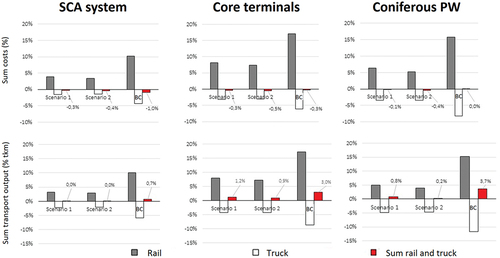
Regardless of system level, the transfer from road to rail decreased as the number of restrictions progressed from optimization of the base case (BC) to scenarios 1 and scenario 2. For the core terminals, optimal solutions for both risk mitigation scenarios (Sc1, Sc2) involved a 4–5% reduction of truck output and 7–8% increase in rail output. Achieving these transfers from road to rail were therefore conditions for low cost risk mitigation.

Finally, when compared to the base case, the mitigation scenarios influenced the final stock balance for the different terminals. For the interior terminals, both mitigation scenarios resulted in 5% higher stocks at Krokom and 20% lower stocks at Hoting. Regarding the mid-zone terminals, final stock status at Backe increased by 13 and 2% for scenarios one and two, respectively. Final stock status was unchanged for the Östavall and Bensjö terminals.

Discussion

The case study provided documentation and analysis of seasonal variation and system risks for rail transport under Swedish conditions. This included the seasonal variation typical for northern areas, particularly for the interior zone (67% higher than mid-zone). Regarding system risks, 16–17% of scheduled routes were subject to deviations, often resulting in cancellations due to either insufficient terminal supply or problems with the locomotives or operators. These problems were also most common in the interior zone due to winter operation of diesel locomotives or longer routes requiring more operators. The mitigation scenarios are fully feasible within the current framework of quarterly supply prognosis periods and the annual planning and timetable allocation routines between SCA, the rail operator and Swedish rail authorities. The tested scenarios had only marginal effects on system costs (<1%).

The cost impact of the mitigations were marginal from the scope of the whole system, the core terminals, and the assortment in focus (Figure 6). Two aspects are relevant to discuss when interpreting these results. The first is the study approach to simulating costs. The second is the network structure of the transport system. Regarding the study approach, comparing optimal solutions to simulate relative costs is a common approach (Lukka 1994; Forsberg et al. 2005). In this study the mitigation scenarios were implemented as period-specific restrictions on flows associated with the highest frequencies of cancellations. This approach is perhaps indirect, but offered a feasible path to quantifying mitigation costs on an annual planning horizon. The associated transfer of transport output from road to rail is certainly a desirable direction of development (Nelldal and Kordnejad 2020), however, achieving this transfer may provide additional challenges. Otherwise, long-term optimizations tend to overestimate improvement potentials when lacking of short-term restrictions (Bergdahl et al. 2003). In this study, for example, using four three-month periods does not capture month-specific variations or provide for precise modeling of medium-term challenges such as spring thaw or planned mill maintenance. However, the consistency of the cost impacts at three levels (systems, core terminals and assortment) implies that the explanation for low mitigation costs, at least partially, lies in the network structure.

Regarding the network structure, 11 supply terminals were distributed across a maximum distance of 1400 km. The terminals represent considerable buffer capacities for the northern, central, and southern supply regions. Once at the terminal, supply may be re-routed to alternative mills with limited cost impacts, given the low rail costs per m³km. In principle, the whole system with all terminals could offer 88 alternative rail flows to eight SCA mills. From a supply mitigation perspective, the core terminal network provides six alternative (contingency) supply flows for a single mill. From a consumption perspective, the core terminals had eight potential demand nodes (including external mills, see Figure 1). Assuming three saw mills with similar log quality demands, the core system provides two contingency flows in case of reduced consumption at one mill. From this perspective, the number of contingency flows was inherently higher for supply risks than demand risks. The structural flexibility available in such a system lays the foundation for low mitigation costs.

The network configuration of the studied system can be compared to other similar systems. The Trätåg rail system (https://tratag.se) extends north from southern Sweden and partially overlaps the southern periphery of the SCA system. This system transports approx. 2.8 million m³ between 9–10 supply terminal and 10 mills. Two of the mills served by this system are also fed by a third system; Norgespendeln, which delivers 1.5 million m³ from 10 terminals in Norway (Løfsgaard 2018; Wallheim 2022). While the number of supply terminals is similar for all three examples the varying number of demand nodes reflect varying contingency flows and structural flexibility for demand risks.

Seen from a theoretical perspective, the configuration of these systems can be related to degrees of system control. In the context of logistics systems control describes the capability of the controlling system to meet the different states of the controlled system and its operating environment (Bolin and Hultén 2002). This balance is termed requisite variety (Ashby 1956), where in this case the network structure provides the system regulators (e.g. SCA/RO) with a sufficient range of responses to meet the variations typical of the controlled system.

Achieving increased short-term flexibility – To supplement earlier studies of solution methods for solving freight scheduling, the interviews provide insight into routines for achieving flexibility for roundwood transport in practice. According to the interviews, both mitigation scenarios could be planned and implemented within the existing annual framework for timetable applications with Swedish rail authorities. Further flexibility at a quarterly time horizon was also considered possible, but limited in practice by the possibility to lease additional rolling stock. A more notable result was the theoretical possibility to increase monthly flows by up to 100% through re-allocation of rolling stock between flows with varying distances. In this case, the bottleneck was the additional workload for the RO for re-planning, and was not considered sustainable with frequent re-planning. The mapping also presented options for short-term flexibility at the weekly or daily level. This would enable a high-resolution analysis of costs for short-term responses. In this case the research approach could be developed toward further simulation approach (Kogler and Rauch 2019) with hybrid simulation-optimization to ensure efficient re-planning between numerous contingencies (Marques et al. 2014).

Conclusions

This study examined the seasonal supply and system risks for wood deliveries by rail in mid-Sweden. Seasonal variation was greatest in the interior zone, as were the risks for system disturbances. Mitigation measures for seasonal supply and risks were fully feasible within the existing annual planning and timetable allocation routines for the forest company, rail service operator and rail authorities. The tested responses had only marginal effects on system costs (<1%) due to the structural flexibility offered by the network. However, the solutions involved a 4–5% reduction of truck output and 7–8% increase in rail output.

Acknowledgements

The authors thank Mikael Frisk and Mikael Rönnqvist of Creative Optimization for all the development work with Woodflow which made this study possible.

Disclosure statement

No potential conflict of interest was reported by the author(s).

Additional information

Funding

This work was supported by the Bo Rydins Stiftelse för Vetenskaplig Forskning [F4020].

References

- Alexandersson G, Hultén S. 2008. The Swedish railway deregulation path. Rev Netw Econ. 7:18–36. doi:10.2202/1446-9022.1136.
- Andreasson E. 2018. Utveckling och test av en leverantörsportföljmodell för industriell virkesförsörjning (Development and test of a supplier portfolio method for industrial wood supply). Arbetsrapport 489 2018. Umeå, Sweden: Sveriges lantbruksuniversitet, institutionen för skoglig resurshushållning.
- Ashby WR. 1956. An introduction to cybernetics. London: Chapman & Hall Ltd.
- Bane NOR. 2022. Network statement 2022. https://networkstatement.banenor.no/.
- Bark P. 2017). Future Freight Locomotive for Europe (FFL4E) – D4.1 – transport model. Europa comissionen. TFK & Trafikverket.
- Bark P, Skoglund M. 2008. DUOLOK – enhetligt dragkraftsystem för godstransporter på elektrifierade huvudlinjer och för terminal- eller växlingstjänst på icke elektrifierade spår-, terminal- och bangårdsområden (Unified traction systems for non-electrified freight). (TFK-rapport, 2008:8). Stockholm.
- Bergdahl A, Örtendahl A, Fjeld D. 2003. The economic potential for optimal destination of roundwood in North Sweden – effects of planning horizon and delivery precision. Int J For Eng. 14(1):81–88. doi:10.1080/14942119.2003.10702472.
- Bolin H, Hultén L. 2002. Information exchange and controllability in logistics. Working paper 3. Transport Research Institute.
- Borndörfer R, Füenschuh A, Klug T, Schlang T, Schlechte T, Schüllendorf H. 2013. The freight train routing problem. ZIB-Report 13-36 Konrad-Zuse-Zentrum für Informationstechnik Berlin.
- Brus S, Engström O. 2022. Virkesförsörjning SCA - med analys av Östrandsinvesteringen (Analysis of SCA supply strategy). Student report for SLU course SG0216 Forest industry supply strategy; p. 22.
- Cacchiani V, Caprara A, Toth P. 2010. Scheduling extra freight trains on railway networks. Transp Res Part B. 44(2):215–231. doi:10.1016/j.trb.2009.07.007.
- Cacchiani V, Toth P. 2012. Nominal and robust train timetabling problems. Eur J Oper Res. 219(3):727–737. doi:10.1016/j.ejor.2011.11.003.
- Chopra S, Sodhi MMS. 2004. Managing risk to avoid: supply-chain breakdown. MIT Sloan Manage Rev. 46:1.
- Creative Opimization. 2022. Woodflow - creative optimization. https://creativeoptimization.se/losningar/woodflow/.
- FAO. 2020. Forest resources assessment 2020 main report. Rome: Food and Agriculture Organization of the United Nations.
- Fjeld D, Vääitäinen K, V.Hofsten H, Noreland D, Callesen I, Lazdins A. 2021. A common Nordic-Baltic costing framework for road, rail and sea transport of roundwood. NIBIO Rapport. 7/8; p. 1–27.
- Finnish Transport Infrastructure Agency. 2022. Network statement 2022. https://vavla.fi/en/service-providers/commercial-railway-transport/network-statement.
- Forsberg M, Frisk M, Rönnqvist M. 2005. FlowOpt – a decision support tool for strategic and tactical transportation planning in forestry. Int J For Eng. 16:101–114. doi:10.1080/14942119.2005.10702519.
- Harrod S. 2012. A tutorial on fundamental model structures for railroad timetable optimization. Surv Oper Res Manage Sci. 17(2):85–96. doi:10.1016/j.sorms.2012.08.002.
- Haehn R, Ábrahám E, Nießen N. 2020. Freight train scheduling in railway systems. In: Hermanns H, editor. Measurement, modelling and evaluation of computing systems. Vol. 12040, MMB 2020. Springer, Cham: Lecture Notes in Computer Science; p. 225–241.
- Hedlinger C, Nilsson B, Fjeld D. 2005. Service Divergence in Swedish Round Wood Transport. International Journal of Forest Engineering. 16(2):153–166. doi:10.1080/14942119.2005.10702523.
- Innofreight. 2021. Smart Gigawood. Product information. www.innofreight.com.
- Kogler C, Rauch P. 2019. A discrete-event simulation model to test multimodal strategies for a greener and more resilient wood supply. Can J For Res. 49(10):1298–1310. doi:10.1139/cjfr-2018-0542.
- Korbaa O, Boufaied A, Lajimi C. 2017. Assessing and modelling transport delays risk in supply chains. Int J Adv Oper Manage. 9:4. doi:10.1504/IJAOM.2017.089980.
- Larsson K. 2016. Wheel damage and maintenance of SCA Skog wagons [Master of science thesis]. Stockholm (Sweden): KTH Royal institute of technology.
- Lindfeldt A. 2015. Railway capacity analysis – methods for simulation and evaluation of timetables, delays and infrastructure Doctoral thesis in infrastructure. KTH TRITA-TSC-PHD15–002.
- Lukka A. 1994. Materials acquisition planning models. Lappeenranta, Finland: Lappeenranta University of Technology. Research report.
- Lundqvist S, Peterson T. 2008. Risks in the Swedish forest, paper and packaging industry. Jönköping, Sweden: Jönköping International Business School.
- Løfsgaard PAA. 2018. Kartlegging av volumvariasjon per vogn for jernbaneleveranse av massevirke via “Norgespendelen” (Assessment of volume variation per wagon for pulpwood deliveries by rail). Masterarbete 2018, Fakultet for miljövitenskap og naturforvaltning. Norges miljø- og biovitenskapelige universitet.
- Markolf SA, Hoehne C, Fraser A, Chester MV, Underwood BS. 2019. Transportation resilience to climate change and extreme weather events – beyond risk and robustness. Transp Policy. 74:174–186. doi:10.1016/j.tranpol.2018.11.003.
- Marques AF, de Sousa JP, Rönnqvist M, Jafe R. 2014. Combining optimization and simulation tools for short-term planning of forest operations. Scand J For Res. 29(1):166–177. doi:10.1080/02827581.2013.856937.
- Mattsson SA. 2012. Logistik i försörjningskedjor. Lund, Sweden: Studentlitteratur.
- Mattsson L-G, Jenelius E. 2015. Vulnerability and resilience of transport systems – a discussion of recent research. Transp Res Part A Policy Pract. 81:16–34. doi:10.1016/j.tra.2015.06.002.
- Nelldal B-L, Kordnejad B. 2020. Hinder och möjligheter för överföring av godstransporter från väg till järnväg (Hinders and potentials for transfer of freight traffic from road to rail). KTH Rapport TRITA-ABE-RPT-215. Avdelning för transportplanering KTH.
- Saranen J, Hilmola O. 2007. Evaluating the competitiveness of railways in timber transports with discrete-event simulation. Vol. 1(4). World Review of Intermodal Transportation Research; p. 445–458.
- Ta C, Goodchild AV, Pitera K. 2009. Structuring a definition of resilience for the freight transportation system. Transp Res Rec. 2097(1):19–25. doi:10.3141/2097-03.
- Trafikverket. 2022. Network statement 2022. https://bransch.trafikverket.se.
- Trouche G. 2009. Activity-based rail freight costing – a model for calculating transport costs in different production systems Doctoral thesis in railway traffic planning. KTH.
- Wallheim S. 2022. Effekten av dual-mode lokomotiv på transportkostnad för försörjningssystem med ofullständig elektrifiering (The effect of dual-mode locomotives on transport cost for supply chains with incomplete electrification). Rapport från Institutionen för skogens biomaterial och teknologi. 2022: 3 Umeå 2022.