Modelling forest road trafficability with satellite-based soil moisture variables

ABSTRACT

Recent decades have seen increased temperatures and precipitation in the Nordic countries with long-term projections for reduced frost duration and depth. The consequence of these trends has been a gradual shift of delivery volumes to the frost-free season, requiring more agile management to exploit suitable weather conditions. Bearing capacity and trafficability are dependent on soil moisture state and in this context two satellite missions offer potenially useful information on soil moisture levels; NASA’s SMAP (Soil Moisture Active Passive) and ESA’s Sentinel-1. The goal of this pilot study was to quantify the performance of such satellite-based soil moisture variables for modeling forest road bearing capacity (e-module) during the frost-free season. The study was based on post-transport registrations of 103 forest road segments on the coastal and interior side of the Scandinavian mountain range. The analysis focused on roads of three types of surface deposits. Weekly SMAP soil moisture values better explained the variation in road e-module than soil water index (SWI) derived from Sentinel-1. Soil Water Index (SWI), however, reflected the weather conditions typical for operations on the respective surface deposit types. Regression analysis using (i) SMAP-based soil dryness index and (ii) its interaction with surface deposit types, together with (iii) the ratio between a combined SMAP_SWI dryness index and segment-specific depth to water (DTW) explained over 70% of the variation in road e-module. The results indicate a future potential to monitor road trafficability over large supply areas on a weekly level, given further refinement of study methods and variables for improved prediction.

KEYWORDS:

• Bearing capacity
• LFWD
• satellite radar
• climate change

Introduction

The pace of wood supply from the forest to mill varies with regional seasonality. Snow and frost enable access to soft sites while deeper winter snows limit forest operations in montane areas. Operations can also be limited by low winter temperatures in the sub-arctic zone and high precipitation in the oceanic zone. Recent decades have seen an increase in temperature and precipitation (MET 2017; IPCC 2022) in northern Europe. Long-term projections of snow cover, soil moisture and soil frost show a continued trend toward reduced frost duration and depth in the north (Kellomäki et al. 2010). Trends for snow depth, however, interact with winter precipitation levels and are more area-specific. Similar interactions have been shown for long-term development of sea-ice conditions (Jevrejeva et al. 2004) in the Baltic region. The most apparent consequence of these trends has been an increasing proportion of operations during the frost-free season. For lowland areas, which no longer receive sufficient frost or snow, a more agile management has been required to schedule site types to suitable weather conditions. This study examines the potential of satellite-based soil moisture data to support agility in transport management.

In Nordic wood supply, a number of general management approaches have provided a framework for resilience to seasonal variation. At the operational level (i) managers rely on seasonal site trafficability classifications to schedule operations. At the tactical level (ii) supply organizations can exploit the progression of seasonal conditions between climate zones to re-allocate capacity. Exploiting the resulting geographic variation in wood availability then requires strategic investments (iii) linking supply regions and mills with multimodal infrastructure for more flexible and cost-efficient long-distance transport (Sjölling et al. 2023). Utilizing the potential within these approaches requires insight into local operating conditions, their regional distributions, as well as seasonal progression between supply zones.

Bearing capacity and trafficability

From the perspective of wood supply, the balance between annual volumes per trafficability class and the duration of the respective seasons determines the potential to maintain an even capacity utilization and delivery pace. Trafficability reflects the minimum bearing capacity required to avoid soil rutting or road deformation, often assuming a typical transport volume. Classifications of terrain trafficability generally express the highest soil moisture state which a site can withstand without unacceptable rutting or road deformation. Field classifications for harvesting have typically been based on factors such as surface deposit types, textures and soil moisture regimes as indicated by forest vegetation classes (Berg et al. 1991). Corresponding military classifications for off-road mobility have often relied on standardized measures for the respective soil friction or cohesion characteristics (McCullough et al. 2017; Choi et al. 2018). For forest roads trafficability classifications are specified through national road construction guidelines (e.g. Metsäteho 2001; LMD 2013; Skogsstyrelsen 2011). Both terrain and road trafficability, however, are often linked by the underlying quaternary surface deposit types. Road trafficability classification has been more common for company forests (Stridsman 2006) since road construction data has been difficult to compile for nonindustrial private forest holdings (Biometria 2021). One common alternative for measuring bearing capacity on public roads has been the falling weight deflectometer (Lenngren and Mårtensson 2003), however during recent years lightweight deflectometers have also been tested on forest roads (Kaakkurivaara and Uusitalo 2015; Tvengsberg 2016). These methods have also been supplemented with road surface laser scanning and ground-penetrating radar to more accurately estimate segment-specific bearing capacity (Christoffersson and Johansson 2012). Recent studies have also tested the use of high-resolution soil moisture maps for improved estimation of bearing capacity for individual road segments (Johannessen 2017).

Transport management

In practice the number of road trafficability classes often vary from 2–4, depending on the context. Scheduling of operations during the frost-free season can be done either by necessity (e.g. wet conditions when only the highest trafficability class is sufficient) or by opportunity (e.g. dry conditions when lower trafficability classes may be used). As much of the variation in operating conditions is temperature-driven, seasonality follows the annual solar cycle with transitions marked by solstice and equinox. Together with the typical precipitation levels for the respective regions (e.g. early summer drought or autumn rains) these provide the typical framework for manager experience and local knowledge. General trends for seasonal variation of bearing capacity on public roads is presented by Aurstad et al. (2016), and similar patterns have been shown using light-weight deflectometers (e-module in MPa) for forest roads (Fjeld et al. 2022). Fjeld et al. (2021, 2022) also tested tracking of individual truck loads via digital transport messaging to infer the effects of temperature and precipitation on trafficability. The inference approach reflected how transport managers and hauling contractors scheduled transport from different site/road types under varying weather conditions. Corresponding transport lead times (time from harvesting to delivery) have been linked to surface deposit types and their respective permeabilities (Maagaard 2021). Overall, difficult weather and reduced forest road trafficability are in the two top-ranked challenges both for impact on wood supply and for work intensity for transport managers (Sterner et al. 2023).

Approaches to trafficability modelling

For harvesting and forwarding, high-resolution soil moisture maps have proven to provide effective decision support for both operators and managers (Flisberg et al. 2020; Sjöberg 2022). These may also be relevant for forest roads since they represent the road subgrade. The original products (Murphy et al. 2009; Ågren et al. 2014), based on hydrologic modeling of various soil textures in digital terrain models have represented a static product. However, online hydrologic modeling of variables such as relative depth to groundwater or soil saturation levels (www.SeNorge.no) provide an indication of temporal variation in soil moisture levels (daily), but at a lower spatial resolution (1 × 1 km). Such models offer the potential to combine static models with dynamic variation of soil moisture levels (Fjeld et al. 2018). A recent Finnish-Swedish innovation challenge (KvarkenSat 2022) investigated a related principle to utilize soil moisture estimates from satellite-based data for forest operations, where the winning participants (Schönauer 2022) tested a proof-of-concept integrating static soil moisture maps (2 × 2 m) with daily soil moisture index from ERA5–Land data (9 × 9 km) to match in-situ measurements of soil water content.

Satellite radar interpretation is one of the few alternatives which offer cost-efficient and high frequency monitoring of soil moisture over wide areas (Peng et al. 2021), which makes them potentially ideal for wood supply organizations sourcing raw materials from diverse geographies. The advantage lies in using multitemporal radar images (Askne et al. 2003; Santoro et al. 2013; Santoro et al. 2015; Rodríguez-Veiga et al. 2019) which can be acquired regardless of weather conditions. The principle is based on the extraction of radar backscatter, where variation over time can be related to variation in soil moisture levels, which drive bearing capacity. Key factors affecting the backscatter include the vegetation structure, viewing geometry, wavelength and surface roughness (depending on radar wavelength) and dielectric constant. The dielectric constant depends on the moisture content of an object, i.e. in this case the moisture content of the trees, forest soil and potentially roads. Long wavelength radar remote sensing, particularly the L-band (wavelength ≈25 cm) in contrast to shorter wavelength such as C-band (wavelength ≈6 cm), is capable of penetrating vegetation and interacting with the water in the upper soil layers. The longer the wavelength used the deeper the soil will be penetrated by the radar signal.

Both ESA and NASA have had satellite programs for monitoring global soil moisture levels, primarily for agricultural purposes (Table 1). Daily Surface Soil Moisture (SSM_1; 1 × 1 km) has been produced by using ESA Sentinel-1A/1B C-band Synthetic Aperture Radar (SAR) data (Bauer-Marschallinger et al. 2019). SSM from Sentinel-1 is based on a change detection model using the backscatter. The model relies on the assumption that differences in backscatter between two satellite images are only due to changes in soil moisture, and that other surface properties which normally affect backscatter, such as vegetation structure, viewing geometry and surface roughness are static. A further development of SSM is the Soil Water Index (SWI), which utilizes the high temporal resolution of MetOp ASCAT (1 day) and the high spatial resolution of Sentinel-1A/1B (20 m). The NASA Soil Moisture Active Passive (SMAP) satellite mission (Entekhabi et al. 2010) provides products including daily composites of soil moisture and freeze/thaw state available in three grid-spacings: 36, 9, and 3 km. However, only the passive radiometer (L-band) is currently functional and the 3 km products are no longer available.

Table 1. Summary of surface soil moisture (SSM), soil water index (SWI) and NASA-USDA Enhanced SMAP Global soil moisture data (GSMD) products from ESA (European space agency) and NASA (National Aeronautics and Space Administration) satellite missions.

Product name	Satellite mission	Space agency	Temporal resolution (days)	Grid spacing (km)	Band
SSM	Sentinel-1	ESA	2–3	1	C
SWI	Sentinel-1/MetOp	ESA	1	1	C
NASA-USDA Enhanced SMAP GSMD	SMAP	NASA	2–3	10	L

The latest validation of SMAP soil moisture products is presented by Colliander et al. (2022). A joint assimilation of SMAP and Sentinel-1 observations has been reported to perform well toward increasing the spatiotemporal accuracy of soil moisture estimates (Lievens et al. 2017). Global evaluations comparing SMAP (9 km) and SMAP/Sentinel-1 (3 km) showed a close agreement between the two and in-situ soil moisture measurements (Mohseni et al. 2022). Further evaluations of SMAP soil moisture retrieval accuracy for a boreal forest case study are provided by Ambadan et al. (2022).

Development paths for forest operations

Benton et al. (1983) showed preliminary evidence of the potential advantages of multiband imaging radar over photoanalysis for determination of mobility and trafficability in forested areas. An early evaluation of the potential to use SMAP L-3 soil moisture data to calculate soil strength for military maneuver planning was reported by Frankenstein et al. (2015). Stevens et al. (2016) compared off-road vehicle mobility predictions using soil moisture variables from WindSat, NASA Land Information System (LIS) and in-situ soil moisture sensors, including examples of how errors in soil moisture affected errors in off-road mobility predictions.

As noted in the above studies, numerous development paths exist for monitoring weather-driven road trafficability for transport management. One promising path is the use of satellite-based soil moisture data to improve trafficability prediction over diverse supply geographies. Dynamic modeling of road trafficability may be more complex than terrain with the modifying effects of road construction standards and materials over the subgrade, however, the majority of deliveries in the Nordic countries start on unclassified forest roads on nonindustrial private holdings. Improved methods for monitoring of trafficability of unclassified roads in near real-time would provide additional insight for local transport managers and an overview for wood supply managers.

Goal

The goal of the study was to quantify the performance of common satellite-sourced soil moisture products for modeling forest road bearing capacity (e-module) during the frost-free season. The soil moisture products were limited to NASA-USDA Enhanced SMAP Global Soil Moisture Data and ESA’s Sentinel-1 based Surface Soil Moisture (SSM) and Soil Wetness Index (SWI).

Materials and methods

The work was done in three steps. It started with (i) mapping of the relationships between the respective soil moisture variables for clustering, before (ii) examining the drainage of the respective road types in relation to the soil moisture variables for the surrounding area, and (iii) analysis of the effect of the soil moisture variables on road bearing capacity. Drainage and bearing capacity were examined in relation to the subgrade type, road construction materials and their corresponding parameters.

The materials for this study originate from a pilot study with data collection during 2019–2021 across the coastal-interior gradient west and east of the Scandinavian mountain range in Norway. The study design is presented in Fjeld et al. (2022) including field data collection routines and earlier results on measured bearing capacity and road deformation after completed hauling. This article reports the results from re-analysis of the same material using satellite-based soil moisture variables. The original study sampled 33 roads along the coast and 33 roads in the interior. The primary selection criteria was to achieve a balance between the most common quaternary surface deposit types and sampling was limited to recently completed hauling assignments during the frost-free season (weeks 12 to 49).

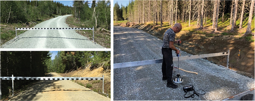
Data collection started with visual inspection of the whole road to select three sample cross-sections corresponding to the segments with least, most and typical rutting. Collection per cross-section started with the measurement of the cross-section profile every 10 cm from a leveled beam with a standard construction laser (Figure 1). A thin transect was excavated on each edge of the cross-section from the wearing course to the ditch to record bearing layer thicknesses and material classification (crushed rock, crushed surface deposits, sorted surface deposits and untreated (native) surface deposits). Bearing layer soil moisture content (volumetric) was measured with a hand-held hygrometer probe at mid-height of the bearing layer. Road bearing capacity (e-module in MPa) was measured on the road surface in each wheel track and at the center line with a Zorn ZPG 3.0 lightweight falling weight deflectometer (LFWD). The model used had a 10 kg falling weight and was designed to measure e-modules up to 60 MPa to a maximum depth of 60 cm. Each sample point had a GPS-coordinate and time stamp to facilitate later joining with other map-based variables. The soil surface deposit type for the subgrade and surrounding terrain was taken from the National Geological Survey (NGU 2015). Depth to water indexes (DTW, cm) were calculated according to Murphy et al. (2009), however, the availability of this data was limited at the time of the study.

Figure 1. Examples of sampled forest road cross-sections, showing 5 m profile beam at left and measurement of e-module at right (Zorn ZPG 3.0 light-weight falling weight deflectometer). E-module was measured in each wheel track and on the uncompacted center line. Photos: Martin Bråthen.

Sentinel-1 SSM and SWI data were made available from the Copernicus Global Land Service (https://land.copernicus.eu/) and a time series of daily data for 2020 and 2021 was downloaded (retrieval date 5 January 2023). The time series of the SMAP data set for 2020 and 2021 was retrieved from Google Earth Engine (retrieval date 5 January 2023). In this study, The NASA-USDA Enhanced SMAP Global Soil Moisture Data at 10 km grid spacing (which will henceforth be referred to as SMAP) was used. This data set is produced by utilizing oversampling of the radiometer to improve the spatial resolution (O’Neill et al. 2016). An explanation of the abbreviations used in the following text is provided in Table 2.

Table 2. List of abbreviations.

Abbreviation	Description
L-band	Radar wavelength of 15–30 cm
C-band	Radar wavelength of 3.8–7.5 cm
SSM	Surface Soil Moisture (%)
SWI_x	Soil water index (%) at soil depth × (cm)
SMAP	NASA-USDA Enhanced SMAP Global Soil Moisture Data (mm)
sfc	Surface
sub	Subsurface
DTW	Depth to water index (cm)
VMC	In-situ measured volumetric soil moisture content (%)
LFWD	Lightweight falling weight deflectometer
e-module	Modulus of elasticity (MPa)

For each road segment, satellite acquisition dates close to the sampling date (target date) were collected. Acquisition dates within 7 days from the target data was filtered for each road segment to provide a weekly mean based on the most recent observation to the target date. Since December 23, 2021 Sentinel-1B has been out of use, but this did not limit the study as all in-situ observations were carried out earlier than this date. Satellite data processing was carried in R (R Core Team, 2022) with statistical analysis in Minitab 18 (www.Minitab-com). Multivariate analysis was used for the introductory mapping of the relationships between dependent and independent variables (clustering and principal component analysis). Conventional linear regression was used for the subsequent analysis of drainage and bearing capacity. An F-test provided the levels of statistical significance for the respective prediction variables on drainage and bearing capacity (p < 0.05*, p < 0.01**, p < 0.001***). Variables with a variation inflation factor (VIF) higher than five were not accepted in the final model.

The total available number of observations (i.e. road cross-sections) was 167. The subsequent analysis of bearing capacity was limited to three categories of surface soil deposits according to their permeability characteristics; glacio-fluvial (high), thick moraine (medium) and ocean or fjord sediment (low). In practice, glacio-fluvial sites are typically reserved for operations during the spring thaw while ocean/fjord sediment sites are reserved for frozen or dry conditions (Fjeld et al. 2022). This provided 103 observations with SSM/SWI/SMAP data and 73 observations with DTW data. The number of observations per surface deposit type is shown in Table 3.

Table 3. The number of observations with DTW and SSM/SWI/SMAP data for the three surface deposit types.

Surface deposit type			No. observations with data
NGU code	Name	Permeability	DTW	SSM/SWI/SMAP
11	Thick moraine deposit	Medium	44	65
20	Glacio-fluvial deposit	High	16	21
41	Ocean/fjord deposit	Low	13	17
Total			73	103

Results

Clustering of soil moisture variables

The respective soil moisture variables (SSM, SWI, SMAP) provided indices of volumetric soil moisture at varying soil depths. SWI provides estimates for depths of 2, 5, 10, 15, 20, 40, 60, and 100 cm, whereas SSM provides estimates for surface soil moisture. SMAP provides estimates for surface and subsurface soil moisture. The variables were clustered according to their similarity in multivariate correlations (Figure 2).

Figure 2. Dendrogram for multivariate clustering of the respective weekly satellite-based soil moisture variables, according to their similarity (%).

The SWI variables were initially reduced to two SWI clusters; SWI surface (95% similarity for SWI_002 to SWI_010) and SWI subsurface (93% similarity for SWI_015 – SWI_100). SMAP surface and SMAP subsurface variables had only 78% similarity and were therefore also kept separate. SSM had 71% similarity with the entire SWI cluster and 40% similarity with the SMAP cluster.

Bearing layer moisture content

The mean e-module varied between categories of bearing layer materials (Table 4). The highest number of observations was for untreated local surface deposits (n = 52), which also had the lowest mean e-module (39,4 MPa) and largest coefficient of variation (CV = 48%). The remainder of the analysis was focused on the untreated (native) surface deposits.

For untreated surface deposits, the drainage of the bearing layer was reflected by the ratios between the in-situ measured volumetric moisture content (VMC%) and the satellite-sourced soil moisture variables (SSM, SWI, SMAP). This ratio varied between surface deposit types (Table 5). The general trend was consistent for most of the soil moisture variables with the lowest ratios for glacio-fluvial deposits (coarse texture) and highest ratios for ocean/fjord sediments (fine texture). For SWI_sfc and SWI_sub, however, the ratios were similar for thick moraines and ocean/fjord sediments.

Visual inspection of scatterplots between the VMC/SMAP ratios and bearing layer thickness showed higher VMC/SMAP ratios for thinner bearing layers, as expected. The slope of this relationship was highest for fine-textured surface deposits (ocean/fjord sediment) and lowest for coarse-textured surface deposits (glacio-fluvial). A linear regression analysis explained 69–73% of the variation using the inverse of bearing layer thickness (dm) and its interaction with surface deposit type (Eqs. 1(1) $\frac{\mathit{VMC}}{\mathit{SMA}{\mathit{P}}_{\mathit{sfc}}}=\mathit{\hspace{0.17em}}-16.52\mathit{\hspace{0.17em}}{\left(\frac{1}{\mathit{layer}\mathit{\hspace{0.17em}}\mathit{thickness}}\right)}^{\ast \ast \ast }+18.33\mathit{\hspace{0.17em}}\left(\frac{1}{\mathit{layer}\mathit{\hspace{0.17em}}\mathit{thickness}}\right)\mathit{moisture}\mathit{\hspace{0.17em}}\mathit{inde}{x}^{\ast \ast \ast }\mathit{\hspace{0.17em}}$(1) and 2(2) $\frac{\mathit{VMC}}{\mathit{SMA}{\mathit{P}}_{\mathit{sub}}}=\mathit{\hspace{0.17em}}-11.75\mathit{\hspace{0.17em}}{\left(\frac{1}{\mathit{layer}\mathit{\hspace{0.17em}}\mathit{thickness}}\right)}^{\ast \ast \ast }+13.47\mathit{\hspace{0.17em}}\left(\frac{1}{\mathit{layer}\mathit{\hspace{0.17em}}\mathit{thickness}}\right)\mathit{moisture}\mathit{\hspace{0.17em}}\mathit{inde}{x}^{\ast \ast \ast }\mathit{\hspace{0.17em}}$(2) ). In this case the deposit type was represented by a moisture index reflecting the relative increase in the mean VMC/SMAP ratios from Table 5 (1.00 for glacio-fluvial deposits, 1.79 for thick moraines and 3.52 for ocean/fjord sediments).

(1) $\frac{\mathit{VMC}}{\mathit{SMA}{\mathit{P}}_{\mathit{sfc}}}=\mathit{\hspace{0.17em}}-16.52\mathit{\hspace{0.17em}}{\left(\frac{1}{\mathit{layer}\mathit{\hspace{0.17em}}\mathit{thickness}}\right)}^{\ast \ast \ast }+18.33\mathit{\hspace{0.17em}}\left(\frac{1}{\mathit{layer}\mathit{\hspace{0.17em}}\mathit{thickness}}\right)\mathit{moisture}\mathit{\hspace{0.17em}}\mathit{inde}{x}^{\ast \ast \ast }\mathit{\hspace{0.17em}}$(1)

R² = 69% adj. R² = 68% n = 51

(2) $\frac{\mathit{VMC}}{\mathit{SMA}{\mathit{P}}_{\mathit{sub}}}=\mathit{\hspace{0.17em}}-11.75\mathit{\hspace{0.17em}}{\left(\frac{1}{\mathit{layer}\mathit{\hspace{0.17em}}\mathit{thickness}}\right)}^{\ast \ast \ast }+13.47\mathit{\hspace{0.17em}}\left(\frac{1}{\mathit{layer}\mathit{\hspace{0.17em}}\mathit{thickness}}\right)\mathit{moisture}\mathit{\hspace{0.17em}}\mathit{inde}{x}^{\ast \ast \ast }\mathit{\hspace{0.17em}}$(2)

R² = 73% adj. R² = 72% n = 51

The intercepts were not significant in the initial analysis and were therefore removed before the final analysis providing Eqs. 1(1) $\frac{\mathit{VMC}}{\mathit{SMA}{\mathit{P}}_{\mathit{sfc}}}=\mathit{\hspace{0.17em}}-16.52\mathit{\hspace{0.17em}}{\left(\frac{1}{\mathit{layer}\mathit{\hspace{0.17em}}\mathit{thickness}}\right)}^{\ast \ast \ast }+18.33\mathit{\hspace{0.17em}}\left(\frac{1}{\mathit{layer}\mathit{\hspace{0.17em}}\mathit{thickness}}\right)\mathit{moisture}\mathit{\hspace{0.17em}}\mathit{inde}{x}^{\ast \ast \ast }\mathit{\hspace{0.17em}}$(1) and 2(2) $\frac{\mathit{VMC}}{\mathit{SMA}{\mathit{P}}_{\mathit{sub}}}=\mathit{\hspace{0.17em}}-11.75\mathit{\hspace{0.17em}}{\left(\frac{1}{\mathit{layer}\mathit{\hspace{0.17em}}\mathit{thickness}}\right)}^{\ast \ast \ast }+13.47\mathit{\hspace{0.17em}}\left(\frac{1}{\mathit{layer}\mathit{\hspace{0.17em}}\mathit{thickness}}\right)\mathit{moisture}\mathit{\hspace{0.17em}}\mathit{inde}{x}^{\ast \ast \ast }\mathit{\hspace{0.17em}}$(2) . Essentially, the ratios between VMC and SMAP just relate the measured bearing layer moisture content to the satellite-based values for the surrounding area, and confirm that the drainage of the bearing layer was poorest for thinner bearing layers of low permeability.

Road bearing capacity

Bearing capacity per cross-section was measured in both the wheel track and center line to reflect compaction after transport. The ratios between e-modules for wheel track and center line were highest for ocean/fjord sediments and lowest for glacio-fluvial deposits (Table 6). The mean e-modules were highest for roads of glacio-fluvial deposits (43.2 and 57.3 MPa for center line and wheel track, respectively. In contrast to values for the center line, the mean e-module in the wheel tracks was slightly lower for thick moraines (34.8 MPa) than for ocean/fjord sediments (37.4 MPa).

Table 4. Mean road bearing capacity (e-module in MPa) per bearing layer material with the variability within each material class (Q1, Q2, CV).

	E-module (MPa in wheel-track)
Bearing layer material	Mean	Q1	Q2	CV (%)	n
Crushed rock	68.6	51	81	28	12
Sorted surface deposit	42.3	34	52	38	29
Untreated surface deposit	39.4	27	52	48	52

Table 5. Ratios between in-situ measured volumetric soil moisture (VMC, %) and satellite-based soil moisture variables SSM, SWI and SMAP (mean, Q1–Q3). Road bearing layers of untreated surface deposits during the frost-free season.

Ratios between soil moisture variables	Glacio-fluvial	Thick moraine	Ocean/fjord
VMC/SSM	0.49 (0.38–0.55)	0.58 (0.49–0.69)	0.71 (0.47–0.86)
VMC/SWI_sfc	0.62 (0.52–0.72)	0.85 (0.71–0.95)	0.83 (0.67–0.99)
VMC/SWI_sub	0.42 (0.38–0.48)	0.57 (0.50–0.63)	0.58 (0.47–0.79)
VMC/SMAP_sfc	3.73 (1.55–5.18)	6.70 (2.59–8.11)	17.66 (1.67–28.06)
VMC/SMAP_sub	3.17 (1.83–4.78)	5.64 (1.78–7.91)	14.00 (1.53–23.81)

Table 6. Mean e-module in road center line and wheel track (MPa) with their ratio (wheel track/center line) with variability in the wheel track (Q1, Q3). Road cross-sections of untreated surface deposits during the frost-free season.

Surface deposit	Center line (MPa)	Wheel track (MPa)	Track/center	Q1	Q3	n
Glacio-fluvial	43.2	57.3	1.32	40.2	67.0	12
Thick moraine	25.4	34.8	1.37	26.6	43.3	24
Ocean/fjord sediment	24.3	37.4	1.54	25.0	48.0	15

A multivariate principal component analysis (PCA) was used to overview the correlations between road bearing capacity, surface deposit categories and satellite-based soil moisture variables. For this analysis the surface deposits were represented with integers for permeability categories (1=low; ocean/fjord sediment, 2=medium; thick moraine, 3=high; glacio-fluvial). The first principal component captured 35% of the total variation, while the first (x-axis) and second (y-axis) captured 64% together. Figure 3 presents the loadings for the respective variables.

Figure 3. Principal component analysis (PCA) loading diagram showing the covariation between road bearing capacity (e-module), surface deposit (SfcDep) permeability and satellite-based soil moisture variables (C-band: SSM, SWI;L-band: SMAP). Road cross-sections of untreated surface deposits during the frost-free season.

The variables with the highest loadings in the first principal component were the SWI variables (0.538–0.540), followed by surface deposit permeability (0.421) and SSM (0.378). The first component appears to capture an association between high SWI soil moisture levels and post-transport registrations on high permeability deposits (3=glacio-fluvial). The variables with the highest loading for the second principal component were the SMAP soil moisture (−0.547 to −0.572) followed by e-module (0.404 to 0.409). High SMAP soil moisture levels were negatively correlated to road bearing capacity (e-module). This is in contrast to a weaker positive loading for bearing capacity (0.158–0.265) in the first component, possibly driven by the association between high SWI and post-transport registrations on high permeability deposits. A graphical comparison of SWI soil moisture levels for each of the surface deposit categories is shown in Figure 4.

Figure 4. Box-plot of SWI soil moisture levels (Swi_sfc, SWI_sub) per permeability category (1=ocean/fjord sediment, 2=thick moraine, 3=glacio-fluvial). Post-transport registrations of untreated surface deposits during the frost-free season.

The above overview provided some insights on how the three soil moisture variables could reflect operating conditions, indicating the possibility that SMAP and SWI may provide complementary aspects of operating conditions. The next step then was to quantify how these variables performed in explaining road e-module. This was done with regression analysis where the dependent variable (e-module_road) consisted of the mean e-module for both wheel tracks and center line. The independent variables used were the mean values of surface (sfc) and sub-surface (sub) moisture for SMAP and SWI, respectively. The initial simple regression analysis for the respective moisture variables (Table 7) included each surface deposit category (SfcDep) without interactions between moisture levels and surface deposits. The scale of the soil moisture variables were reversed to reflect how dry operating conditions were (maximum threshold minus observed moisture value). The following regression analyses were limited to observations with maximum road inclination of 7% and bearing layer thickness of 5 dm.

Table 7. An initial simple regression analysis comparing the effects of alternative soil moisture variables on road e-module (e-module_road in MPa, p < 0.05*, p < 0.01**, p< 0.001***). Road cross-sections of untreated surface deposits during the frost-free season.

Intercept for surface deposit (SfcDep***)			Effect of soil moisture	R^2	Adj. R^2	n
Glacio-fluvial	Thick moraine	Ocean/fjord sediments
36.5	14.3	14.4	+0.616 (40–SMAP)**	43	39	45
50.7	29.6	29.1	+0.396 (65–SWI)	29	24	43
48.7	25.8	20.8	+0.0337 (40–SMAP) (65–SWI)*	37	32	43

For the initial analysis the most consistently significant predictor for e-module was surface deposit category (p = 0.000 for all three models). The highest R² (39–43%) was provided by the first model using SMAP. The second model had a low R² (24–29%) where SWI did not provide a significant effect (p = 0.51). The third model showed a significant interaction between SMAP and SWI and explained 32–37% of the variation in e-module. The simple regressions resulted in diverging values for the respective intercepts, which represent the e-modules for wet conditions.

For a correct modeling of e-module the main challenge was to capture the effect of soil moisture for different surface deposits. Given the initial regression results (Eqs. 1(1) $\frac{\mathit{VMC}}{\mathit{SMA}{\mathit{P}}_{\mathit{sfc}}}=\mathit{\hspace{0.17em}}-16.52\mathit{\hspace{0.17em}}{\left(\frac{1}{\mathit{layer}\mathit{\hspace{0.17em}}\mathit{thickness}}\right)}^{\ast \ast \ast }+18.33\mathit{\hspace{0.17em}}\left(\frac{1}{\mathit{layer}\mathit{\hspace{0.17em}}\mathit{thickness}}\right)\mathit{moisture}\mathit{\hspace{0.17em}}\mathit{inde}{x}^{\ast \ast \ast }\mathit{\hspace{0.17em}}$(1) and 2(2) $\frac{\mathit{VMC}}{\mathit{SMA}{\mathit{P}}_{\mathit{sub}}}=\mathit{\hspace{0.17em}}-11.75\mathit{\hspace{0.17em}}{\left(\frac{1}{\mathit{layer}\mathit{\hspace{0.17em}}\mathit{thickness}}\right)}^{\ast \ast \ast }+13.47\mathit{\hspace{0.17em}}\left(\frac{1}{\mathit{layer}\mathit{\hspace{0.17em}}\mathit{thickness}}\right)\mathit{moisture}\mathit{\hspace{0.17em}}\mathit{inde}{x}^{\ast \ast \ast }\mathit{\hspace{0.17em}}$(2) ) the primary variable was SMAP, together with its interaction with surface deposit categories. To capture how drier conditions (40–SMAP, i.e. maximum threshold minus observed moisture value) influenced e-modules for varying textures surface deposit categories were represented by a continuous variable. The variable tested was the mean e-module for respective deposit types in their uncompacted state (road center line, see Table 6). A strength index was then scaled in relation to the weakest deposit type (ocean/fjord sediments, strength index = 1.0) so that thick moraines and glacio-fluvial deposits had relative strength indices of 1.05 and 1.78, respectively. Since both the initial PCA and regression indicated that SMAP and SWI may provide complementary information on operating conditions an interaction variable was included, represented by their product so that the highest values reflected the driest conditions for both ((40–SMAP)×(65–SWI)). Figure 5 shows scatter plots for e-modules in relation to this product, for both the uncompacted center line (left) as well as the average for the road surface (right).

Figure 5. Scatter plots of e-module (MPa on y-axis) in relation to satellite-based soil dryness index (combined for SMAP and SWI on x-axis) for the three surface deposit types. (a) Uncompacted road center line (left), and (b) mean for road surface (right).

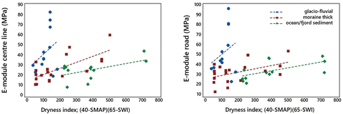
The scatter plot for the uncompacted center line (Figure 5a) shows a more distict progression of e-module for the three surface deposits as conditions became drier. The three highest observations for e-module are above the 60 MPa limit for the deflectometer used and therefore likely to be underestimated.

Following the principles described above two regression analysis were made. The first regression (Eq. 3(3) $\mathit{emodul}{e}_{\mathit{road}}={18.0}^{\ast \ast \ast }-\mathit{\hspace{0.17em}}1.04{\left(40-\mathit{SMAP}\right)}^{\ast \ast }\mathit{\hspace{0.17em}}+\mathit{\hspace{0.17em}}1.31\left(40-\mathit{SMAP}\right)\mathit{\hspace{0.17em}}\mathit{strength}\mathit{\hspace{0.17em}}\mathit{inde}{x}^{\ast \ast \ast }+0.0195\left(40-\mathit{SMAP}\right)\left(65-\mathit{SWI}\right)\mathit{\hspace{0.17em}}$(3) ) explained roughly 50% of the variation in road e-module, but in this case the interaction between SMAP and SWI was not significant. The interaction became significant first when the combined dryness index was seen in relation to depth to water index (DTW, cm) for the specific road cross-section (Eq. 4(4) $\mathit{emodul}{e}_{\mathit{road}}={9.35}^{\ast \ast \ast }-0.892{\left(40-\mathit{SMAP}\right)}^{\ast \ast \ast }+1.52\left(40-\mathit{SMAP}\right)\mathit{\hspace{0.17em}}\mathit{strength}\mathit{\hspace{0.17em}}\mathit{inde}{x}^{\ast \ast \ast }+0.846\frac{\left(40-\mathit{SMAP}\right)\left(65-\mathit{SWI}\right)}{\mathit{DTW}}{\mathit{\hspace{0.17em}}}^{\ast }\mathit{\hspace{0.17em}}$(4) ). The equation could then explain over 70% of the variation in e-module.

(3) $\mathit{emodul}{e}_{\mathit{road}}={18.0}^{\ast \ast \ast }-\mathit{\hspace{0.17em}}1.04{\left(40-\mathit{SMAP}\right)}^{\ast \ast }\mathit{\hspace{0.17em}}+\mathit{\hspace{0.17em}}1.31\left(40-\mathit{SMAP}\right)\mathit{\hspace{0.17em}}\mathit{strength}\mathit{\hspace{0.17em}}\mathit{inde}{x}^{\ast \ast \ast }+0.0195\left(40-\mathit{SMAP}\right)\left(65-\mathit{SWI}\right)\mathit{\hspace{0.17em}}$(3)

R² = 53% adj. R² = 49% n = 43 $\mathit{\hspace{0.17em}}$

(4) $\mathit{emodul}{e}_{\mathit{road}}={9.35}^{\ast \ast \ast }-0.892{\left(40-\mathit{SMAP}\right)}^{\ast \ast \ast }+1.52\left(40-\mathit{SMAP}\right)\mathit{\hspace{0.17em}}\mathit{strength}\mathit{\hspace{0.17em}}\mathit{inde}{x}^{\ast \ast \ast }+0.846\frac{\left(40-\mathit{SMAP}\right)\left(65-\mathit{SWI}\right)}{\mathit{DTW}}{\mathit{\hspace{0.17em}}}^{\ast }\mathit{\hspace{0.17em}}$(4)

R² = 78% adj. R² = 76% n = 32 $\mathit{\hspace{0.17em}}$

where the relative values for mean surface deposit strength were as follows:

$\mathrm{ocean}/\mathrm{fjord}\mathrm{sediments}=1.0;\mathrm{thick}\mathrm{moraine}=1.05;\mathrm{glacio}\text{-}\mathrm{fluvial}=1.78$

The inclusion of DTW in the regression reduced the number of observations to 32 because of the limited DTW coverage at the time of the study. The variation inflation factors (VIF) did not exceed 3.0 for any of the variables.

Discussion

The pilot study provided some general trends relating satellite-based soil moisture variables to weekly variation in forest road bearing capacity. The fundamental relationships such as drainage of the road bearing layer for varying thicknesses and surface deposits were as expected (Eqs. 1(1) $\frac{\mathit{VMC}}{\mathit{SMA}{\mathit{P}}_{\mathit{sfc}}}=\mathit{\hspace{0.17em}}-16.52\mathit{\hspace{0.17em}}{\left(\frac{1}{\mathit{layer}\mathit{\hspace{0.17em}}\mathit{thickness}}\right)}^{\ast \ast \ast }+18.33\mathit{\hspace{0.17em}}\left(\frac{1}{\mathit{layer}\mathit{\hspace{0.17em}}\mathit{thickness}}\right)\mathit{moisture}\mathit{\hspace{0.17em}}\mathit{inde}{x}^{\ast \ast \ast }\mathit{\hspace{0.17em}}$(1) and 2(2) $\frac{\mathit{VMC}}{\mathit{SMA}{\mathit{P}}_{\mathit{sub}}}=\mathit{\hspace{0.17em}}-11.75\mathit{\hspace{0.17em}}{\left(\frac{1}{\mathit{layer}\mathit{\hspace{0.17em}}\mathit{thickness}}\right)}^{\ast \ast \ast }+13.47\mathit{\hspace{0.17em}}\left(\frac{1}{\mathit{layer}\mathit{\hspace{0.17em}}\mathit{thickness}}\right)\mathit{moisture}\mathit{\hspace{0.17em}}\mathit{inde}{x}^{\ast \ast \ast }\mathit{\hspace{0.17em}}$(2) ). However, the modeling of road e-module with SMAP versus SWI presented a slight paradox. Weekly SMAP values generally better explained the variation in e-module (Eqs. 1(1) $\frac{\mathit{VMC}}{\mathit{SMA}{\mathit{P}}_{\mathit{sfc}}}=\mathit{\hspace{0.17em}}-16.52\mathit{\hspace{0.17em}}{\left(\frac{1}{\mathit{layer}\mathit{\hspace{0.17em}}\mathit{thickness}}\right)}^{\ast \ast \ast }+18.33\mathit{\hspace{0.17em}}\left(\frac{1}{\mathit{layer}\mathit{\hspace{0.17em}}\mathit{thickness}}\right)\mathit{moisture}\mathit{\hspace{0.17em}}\mathit{inde}{x}^{\ast \ast \ast }\mathit{\hspace{0.17em}}$(1) -4(4) $\mathit{emodul}{e}_{\mathit{road}}={9.35}^{\ast \ast \ast }-0.892{\left(40-\mathit{SMAP}\right)}^{\ast \ast \ast }+1.52\left(40-\mathit{SMAP}\right)\mathit{\hspace{0.17em}}\mathit{strength}\mathit{\hspace{0.17em}}\mathit{inde}{x}^{\ast \ast \ast }+0.846\frac{\left(40-\mathit{SMAP}\right)\left(65-\mathit{SWI}\right)}{\mathit{DTW}}{\mathit{\hspace{0.17em}}}^{\ast }\mathit{\hspace{0.17em}}$(4) ) while mean SWI values appeared to reflect the weather conditions typical for scheduling of operations on the respective surface deposit types (Figures 3 and 4). A combined SMAP and SWI dryness index provided visually distinct trends for e-module for the respective surface deposits (Figure 5), however this interaction was significant first when related to section-specific DTW index (Eq. 4(4) $\mathit{emodul}{e}_{\mathit{road}}={9.35}^{\ast \ast \ast }-0.892{\left(40-\mathit{SMAP}\right)}^{\ast \ast \ast }+1.52\left(40-\mathit{SMAP}\right)\mathit{\hspace{0.17em}}\mathit{strength}\mathit{\hspace{0.17em}}\mathit{inde}{x}^{\ast \ast \ast }+0.846\frac{\left(40-\mathit{SMAP}\right)\left(65-\mathit{SWI}\right)}{\mathit{DTW}}{\mathit{\hspace{0.17em}}}^{\ast }\mathit{\hspace{0.17em}}$(4) ). All in all, the results of the pilot study point to a future potential to monitor road trafficability over large supply areas at a weekly level, given further refinement of study methods and variables for improved prediction.

Critique of materials and methods

The pilot was originally designed to capture wide scale variation over a gradient from coastal to interior conditions. The selection of the three cross-sections per road was designed to capture the extremes from most to least rutting, presumeably driven by moisture levels in the underlying sub-grade soil. Regarding the LFWD used in this study; a 10 kg model was practical to transport and use in the field, but in hindsight it should have been heavier (e.g. 15 kg) to enable deeper penetration and measurements over 60 MPa. The operating instructions for the Zorn LFWD also assume the use of a layer of sand to provide good contact between the deflection plate and the road surface. In this pilot, however, field workers were just instructed to avoid large stones and even out the contact area with a spade. Earlier comparisons between the LFWD and full-scale FWD have shown systematic errors in LFWDs estimation of bearing capacity (Kaakkurivaara and Uusitalo 2015; Tvengsberg 2016). At the same time, the road deformation reported earlier for the current study was well correlated with e-modules for center line versus wheel tracks (Fjeld et al. 2022). Another potential source of error were the hand-held hygrometers used for in-situ measurements of bearing layer moisture content. These can be inaccurate when being used across a variety of soil textures. The measured values, however, provided a logical progression of drainage between the respective surface deposit types when compared to both surface and subsurface SMAP (Table 5). All in all, the material and methods support the modeling of general trends, but limit the predictive power for management purposes.

Critique of analysis approach

The multivariate clustering of the various satellite-based variables revealed differences between SMAP and SWI, also between different soil depths. In most of the introductory analyses subsurface SMAP proved to be the best predictor for both drainage and e-module, closely followed by surface SMAP. The subsequent focus on roads built with untreated local surface deposits limited the number of observations and motivated the use of more general variables (e.g. averages of surface/subsurface moisture and e-module for the wheel tracks/center line). Since both the PCA (Figure 3, using depth-clustered variables) and the initial simple regression (Table 7, using the mean of surface and subsurface values) indicated that SMAP moisture content was better linked to bearing capacity, SMAP was the primary choice for modeling of interactions with surface deposits.

The approach to modeling e-module with soil moisture and surface deposit interactions followed a structure common for forest operations studies. As an alternative to additive affects, Bergstrand (1987) presents a sunray model for modeling interaction effects between the independent variable and multiple dependent variables. The approach structures interactions as the product of the first independent variable (e.g. SMAP soil dryness; 40–SMAP) with a second independent variable (e.g. surface deposit category and the associated geotechnical propoerties). The sunray approach used ranked integer values to represent categories of the second independent variable (dummy variables). The current study tested replacing the categorical variable with a continuous variable consisting of a geotechnical strength index based on mean soil strengths for the uncompacted surface deposits. One risk associated with this approach is the associated differences in mean SWI moisture levels between surface deposits indicating generally wetter conditions during the post-transport sampling of glacio-fluvial deposits and drier conditions for ocean/fjord deposits (Figure 4). If the SWI values truly reflected operating conditions, the use of the strength index as a continuous variable could have introduced a systematic error in the estimation of moisture effects for coarse versus fine textures. However, since the SMAP-based variables provided a more plausible progression of bearing layer drainage (Table 5) between glacio-fluvial deposits (dry coarse textures) versus ocean/fjord sediments (moist fine textures) this risk seems small.

Adding an interaction between SMAP and SWI dryness levels to the e-module regression (Eqs. 3(3) $\mathit{emodul}{e}_{\mathit{road}}={18.0}^{\ast \ast \ast }-\mathit{\hspace{0.17em}}1.04{\left(40-\mathit{SMAP}\right)}^{\ast \ast }\mathit{\hspace{0.17em}}+\mathit{\hspace{0.17em}}1.31\left(40-\mathit{SMAP}\right)\mathit{\hspace{0.17em}}\mathit{strength}\mathit{\hspace{0.17em}}\mathit{inde}{x}^{\ast \ast \ast }+0.0195\left(40-\mathit{SMAP}\right)\left(65-\mathit{SWI}\right)\mathit{\hspace{0.17em}}$(3) and 4(4) $\mathit{emodul}{e}_{\mathit{road}}={9.35}^{\ast \ast \ast }-0.892{\left(40-\mathit{SMAP}\right)}^{\ast \ast \ast }+1.52\left(40-\mathit{SMAP}\right)\mathit{\hspace{0.17em}}\mathit{strength}\mathit{\hspace{0.17em}}\mathit{inde}{x}^{\ast \ast \ast }+0.846\frac{\left(40-\mathit{SMAP}\right)\left(65-\mathit{SWI}\right)}{\mathit{DTW}}{\mathit{\hspace{0.17em}}}^{\ast }\mathit{\hspace{0.17em}}$(4) ) was of interest since their initial clustering (Figure 2) indicated that they may reflect different aspects of operating conditions. Their product represents a combined index of how dry operating conditions were at the time of sampling. Neither the combined dryness index nor section-specific DTW were significant alone, and it was first when the combined index was seen in relation to DTW that the effects were significant (Eq. 4(4) $\mathit{emodul}{e}_{\mathit{road}}={9.35}^{\ast \ast \ast }-0.892{\left(40-\mathit{SMAP}\right)}^{\ast \ast \ast }+1.52\left(40-\mathit{SMAP}\right)\mathit{\hspace{0.17em}}\mathit{strength}\mathit{\hspace{0.17em}}\mathit{inde}{x}^{\ast \ast \ast }+0.846\frac{\left(40-\mathit{SMAP}\right)\left(65-\mathit{SWI}\right)}{\mathit{DTW}}{\mathit{\hspace{0.17em}}}^{\ast }\mathit{\hspace{0.17em}}$(4) ). Essentially, dividing the combined dryness index (product of 40–SMAP and 65–SWI) with DTW just reduces the effect of dry operating conditions on already dry sections (deep DTW) and increases the effect where water was close to the subgrade surface. This builds on a proof-of-concept presented by Schönauer (2022) for integrating static soil moisture maps (high spatial resolution) with dynamic soil moisture levels from satellite-based variables (low spatial resolution and high temporal resolution). If valid, using DTW in this way could enable identification of bottleneck road sections of lower e-module, assuming otherwise similar construction standards.

Comparison to earlier studies

Considerable investments have been made over time in cross-country and on-road mobility models for military purposes (McCullough et al. 2017). These are rarely referred to in forestry literature, even though many of the underlying variables are related, and these studies have already revealed a potential for improvement with satellite-based soil moisture variables (Frankenstein et al. 2015; Stevens et al. 2016). While these studies are most commonly focused on driving speed, purely static models have also been shown to risk low achievement of indicated speeds (Choi et al. 2018). Most of these models have also been aimed at geograhies with a lower proportion of post-glacial surface deposits and the geotechnical properties associated with high occurrences of larger stones, which have been inherent in Nordic forest operations classifications (cf. Berg et al. 1991). North American road design guidelines have been based on indexes of bearing capacity such as the California Bearing Ratio (CBR) or cone-penetration indices (Bolander et al. 1995; Bradley 2001; Bergqvist et al. 2017) which perform well in deeper stone-free soils. Finnish modeling of seasonal requirements for forest road bearing capacity expresses requirements in terms of e-module, where the latest work (Strandström 2018) provided updated models for calculating road e-module based on layer-specifice-modules (MN/m²) for the respective layer materials and thicknesses. In the Finnish case the bearing capacity requirements were specified as 60–80 MPa for the spring thaw and 50–60 MPa for the rest of the year. Comparing these thresholds to the current study, the only bearing layer material meeting the Finnish spring thaw requirements was crushed rock, while most of the roads of untreated local surface deposits were under 50 MPa, barely fulfilling the the requirements for frost-free periods. The lower bearing capacity for untreated surface deposits in the current study may well be a reflection of the lower transport intensity and generally wetter climate in Norway. However another important factor is the age of the forest road network. The pace of forest road construction in Norway was highest during the 1960s (1000 km/year) and 1970–1990 (800 km/year), falling rapidly to 200 km/year after 2000 (Johannessen 2017). A growing mismatch between older forest roads and increasing truck length and GVWs (76 t in Finland, 74 t in Sweden and most likely an increase from 60 to 68 t in Norway) has resulted in increased pace for upgrading (420 km/year) versus new construction (120 km/year) in Norway.

Management implications and development potential

Upgrading the private road network to meet the new demands for forest logistics is a long-term investment. During this transition, it would be advantageous for haulers and managers to have some objective indication of trafficability over mill supply areas. Combining the static data on road and subgrade with weekly soil moisture data from satellite sources resulted in an acceptable modeling of road section-specific trafficability. Satellite-based soil moisture data from NASA/USDA’s SMAP mission performed best and its performance otherwise is well documented (Colliander et al. 2022; Schönauer et al. 2022). The most plausible explanation for better performance is the longer wavelength (L-band) compared to ESAs Sentinel-1 (C-band) since longer wavelengths generally provide better penetration of precipitation, forest canopies and soil (Santoro et al. 2019; Cohen et al. 2021). However, given the rapid development of new algorithms making use of multiple sources (Peng et al. 2021; Mohseni et al. 2022) new products and predictors are sure to come in the future.

Using satellite-based soil moisture variables to model e-module provides an opportunity to bypass indirect sources based on weather data and wide-scale hydrological modeling. In its simplest form trafficability could be monitored using an e-module curve (e.g. Eq. 4(4) $\mathit{emodul}{e}_{\mathit{road}}={9.35}^{\ast \ast \ast }-0.892{\left(40-\mathit{SMAP}\right)}^{\ast \ast \ast }+1.52\left(40-\mathit{SMAP}\right)\mathit{\hspace{0.17em}}\mathit{strength}\mathit{\hspace{0.17em}}\mathit{inde}{x}^{\ast \ast \ast }+0.846\frac{\left(40-\mathit{SMAP}\right)\left(65-\mathit{SWI}\right)}{\mathit{DTW}}{\mathit{\hspace{0.17em}}}^{\ast }\mathit{\hspace{0.17em}}$(4) ) or table indicating when conditions reach or drop below specified threshold limits. This would provide a solution for the key questions of when fine-textured soils are dry enough to initiate operations (see ocean/fjord sediments in Figure 5 for a graphical example). Further studies, however should include a wider set of surface deposit types with clustering according to geotechnical properties relevant for heavy vehicles. Such work would provide the foundation for fully digital satellite-supported applications, starting with a trafficability or availability index based on e-module thresholds. The trafficability index can then be joined with roadside stock levels to support weekly transport planning at the district level. Aggregation of district-level data provides an improved prognosis for weekly deliveries to mills and multimodal terminals (Sjölling et al. 2023). Such geographically aggregated data would then provide the basis for an early warning function for changing transport conditions and reduced wood availability with a subsequent need to reallocate resources between supply areas. The main risk of such a development is prediction error, which would be first noticed by local haulers, and later by transport or wood supply managers. The amount of data processing which is required for maintaining an updated weekly prediction will be considerable and require automation and system development. Further integration with real-time inferences such as truck diesel consumption (Svenson and Fjeld 2016) and digital transport messaging (Fjeld et al. 2022; Sterner et al. 2023) for self-learning cycles can potentially be facilitated by a combination of automated and augmented AI (Holzinger et al. 2022).

Because of the current trends for reduced winter frost in the north (Kellomäki et al. 2010) this study has focused on modeling bearing capacity during frost-free periods. Freeze/thaw processes in these regions are generally considered troublesome for wood supply management so further development of satellite support functions is also relevant for this purpose. Cohen et al. (2021) presents an approach for daily freeze/thaw estimation in boreal forest environments based on data retrieval from Sentinel-1.

Conclusions

The results show that soil moisture estimates from coarse-resolution radar can provide valuable insight into bearing capacity for forest roads of untreated surface deposits. Modelling e-module with L-band SMAP versus C-band Sentinel-1-based soil moisture variables presented a slight paradox. Weekly SMAP soil moisture values better explained the variation in e-module while mean SWI values derived from Sentinel-1 data appeared to reflect the weather conditions typical for scheduling operations on the respective surface deposit types. Regression analysis using a SMAP-based soil dryness index and its interaction with surface deposit types, together with the ratio between a combined SMAP and SWI dryness index and the section-specific DTW explained over 70% of variation in e-module. The results of the pilot study point to a future potential to monitor road trafficability over large supply areas at a weekly level, given further refinement of study methods and variables for improved prediction.

Acknowledgements

The authors thank Dag Skjølaas of the Federation of Norwegian Forest Owners, the participating forest owners associations (Allskog, Glommen-Mjøsen Skog, Viken Skog, AT-Skog, Vestskog) as well as the respective financiers (Skogtiltaksfondet and Utviklingsfondet for Skogbruket) for making this study possible. We also thank Paul Geladi and Anders Brundin for their help with multivariate analysis.

Disclosure statement

No potential conflict of interest was reported by the authors.

References

- Ågren AM, Lindberg W, Strömgren M, Ogilvie J, Arp PA. 2014. Evaluating digital terrain indices for soil wetness mapping – a Swedish case study. Hydrol Earth Syst Sci. 18(9):3623–3634. doi: 10.5194/hess-18-3623-2014.
- Ambadan JT, MacRae HC, Colliander A, Tetlock E, Helgason W, Gedalof Z, Berg AA. 2022. Evaluation of SMAP Soil Moisture Retrieval Accuracy over a Boreal Forest Region. IEEE Trans Geosci Remote Sens. 60(2022):4414611. doi: 10.1109/TGRS.2022.3212934.
- Askne J, Santoro M, Smith G, Fransson JES. 2003. Multitemporal repeat-pass SAR interferometry of boreal forests. IEEE Trans Geosci Remote Sens. 41(7):1540–1550. doi: 10.1109/TGRS.2003.813397.
- Aurstad J, Aksnes J, Berntsen G, Gryteselv D, Johansen R, Lindland T, Ø M, Oset F, Ottesen HB, Paulsrud G, et al. 2016. Textbook for road technology (bd. 626). Norwegian: Vegdirektoratet.
- Bauer-Marschallinger B, Freeman V, Cao S, Paulik C, Schaufler S, Stachl T, Modanesi S, Massari C, Ciabatta L, Brocca L. 2019. Toward global soil moisture monitoring with Sentinel-1: harnessing assets and overcoming obstacles. IEEE Trans Geosci Remote Sens. 57(1):520–539. doi: 10.1109/TGRS.2018.2858004.
- Benton AR, Blanchard AJ, Newton RW 1983. Determination of mobility and trafficability indicators with multifrequency imaging radar. Proceedings: SPIE 0414 optical engineering for cold environments; Sept 22; Arlington, USA.
- Berg S, Frumerie G, Forshed N. 1991. Terrain classification system for forestry work. Forest Operat Inst Sweden. 1–28.
- Bergqvist M, Bradley A, Björheden R, Eliasson L. 2017. Validation of the surfacing thickness program for Swedish conditions. Skogforsk Arbetsrapport No.920-2017. 1–39.
- Bergstrand K-G. 1987. Planning and analysis of time studies on forest technology. Forest Operat Inst Sweden. 17:1–58.
- Biometria. 2021. Klassning av skogsbilvägar (classification of forest roads). Swedish. (https://www.biometria.se/media/fa1ba4qc/klassning-av-skogsbilvaegar_september2021_webb.pdf).
- Bolander P, Marocco D, Kennedy R. 1995. Earth and aggregate surfacing design guide for low volume roads. Washington: USDA Forest Service; p. 302.
- Bradley A. 2001 October. Evaluation of forest access road design for use with CTI equipped logging trucks. FERIC Advantage. 2(53):1–16.
- Choi KK, Gaul N, Jayakumar P, Wafy TM, Funk M 2018. Framework of reliability-based stochastic mobility map for next generation Nato reference mobility model. Proceedings of the 2018 Ground Vehicle Systems Engineering and Technology Symposium; Aug 7-9; Novi, Michigan. p. 1–15.
- Christoffersson P, Johansson S 2012. Rehabilitation of the timmerleden forest road. A ROADEX demonstration report, the Swedish transport administration, Northern Region, Sweden. 38 pp.
- Cohen J, Rautiainen K, Lemmetyinen J, Smolander T, Vehviläinen J, Pulliainen J. 2021. Sentinel-1 based soil freeze/thaw estimation in boreal forest environments. Remote Sens Environ. 254:112267. doi: 10.1016/j.rse.2020.112267.
- Colliander A, Reichle RH, Crow WT, Cosh MH, Chen F, Chan S, Das NN, Bindlish R, Chaubell J, Seungbum K, et al. 2022. Validation of soil moisture data products from the NASA SMAP mission. IEEE J Sel Top Appl Earth Observat Remote Sens. 15:364–392. doi: 10.1109/JSTARS.2021.3124743.
- Entekhabi D, Njoku EG, O’Neill PE, Kellogg KH, Crow WT, Edelstein WN, Entin JK, Goodman SD, Jackson TJ, Johnson J, et al. 2010. The Soil Moisture Active Passive (SMAP) mission. Proc IEEE. 98(5):704–716. doi: 10.1109/JPROC.2010.2043918.
- Fjeld D, Bjerketvedt J, Fønhus M 2018. Nye muligheter for klassifisering av bæreevne (New possibilities for classifying bearing capacity). Norsk Skogbruk 4-2018: 45–47. Norwegian.
- Fjeld D, Bjerketvedt J, Bråthen M 2021. Forest road availability – inferences from logging truck delivery messages. Proceedings COFE-FORMEC 2021; Sept 27-30; Corvallis, OR. p. 180–183.
- Fjeld D, Bjerketvedt J, Bråthen M, 2022. Baereevneklassifisering av skogsbilveier. Resultater av pilotforsöket 2018-2021 (Bearing capacity classification of forest roads – results of a pilot study). NIBIO Report Vol. 8 No. 147: 41 pp. Norwegian.
- Flisberg P, Rönnqvist M, Willén E, Frisk M, Friberg G. 2020. Spatial optimization of ground-based primary extraction routes using the BestWay decision support system. Can J For Res. 51(5):675–691. doi: 10.1139/cjfr-2020-0238.
- Frankenstein S, Stevens M, Scott C. 2015. Ingestion of simulated SMAP L3 soil moisture data into military maneuver planning. Journal Of Hydrometereol. 16(1):427–440. doi: 10.1175/JHM-D-14-0032.1.
- Holzinger A, Saranti A, Angerschmid A, Retzlaff CO, Gronauer A, Pejakovic V, Medel F, Krexner T, Gollob C, Stampfer K. 2022. Digital Transformation in Smart Farm and forest operations needs human-centered AI: challenges and future directions. Sensors. 22(8):3043. doi: 10.3390/s22083043.
- IPCC. 2022. Sixth assessment report. Working group 1- the physical science basis. Regional fact sheet Europe. (www.ipcc.ch).
- Jevrejeva S, Drabkin VV, Kostjukov J, Lebedev AA, Leppäranta M, Mironov YU, Schmelzer N, Sztobryn M. 2004. Baltic Sea ice seasons in the twentieth century. Clim Res. 25:217–227. doi: 10.3354/cr025217.
- Johannessen KA 2017. Examination of the relationship between soil types, soil moisture and the carrying capacity of roads. Masters thesis NMBU Inst. Natural Resource Management. 51 pp. Norwegian
- Kaakkurivaara T, Uusitalo J. 2015. Applicability of portable tools in assessing the bearing capacity of forest roads. Silva Fenn. 49(2):1239. doi: 10.14214/sf.1239.
- Kellomäki S, Maajärvi M, Strandman H, Kilpeläinen A, Peltola H. 2010. Model computations on the climate change effects on snow cover, soil moisture and soil frost in the boreal conditions over Finland. Silva Fenn. 44(2):213–233. doi: 10.14214/sf.455.
- KvarkenSat 2022. Kvarken Space Center – Enabling New Space Economy in Kvarken. www.kvarkenspacecenter.org.
- Lenngren CA, Mårtensson B 2003. The falling weight deflectometer – an underestimated tool for managing forest road design and maintenance. Proc. 2nd Forest Engineering Conference; May 12-15; Växjö SkogForsk Arbetsrapport 535. p. 129–138.
- Lievens H, Reichle RH, Liu Q, De Lannoy GHM, Dunbar RS, Kim SB, Das NN, Cosh M, Walker JP, Wagner W. 2017. Joint Sentinel-1 and SMAP data assimilation to improve soil moisture estimates. Geophys Res Lett. 44(12):6145–6153. doi: 10.1002/2017GL073904.
- LMD. 2013. Normaler for landbruksveier med byggebeskrivelse (Guidelines for agricultural roads with construction descriptions). Landbruks- og matdepartementet. (http://www.skogkurs.no/vegnormaler)
- Maagaard JS 2021. Transport lead times – a survey of variation and causes. NMBU masters thesis. Faculty for environmental sciences and natural resource management. Norwegian. 35 pp
- McCullough M, Jayakumar P, Dasch J, Gorsich D. 2017. The next generation NATO reference mobility model development. J Terramechanics. 73(2017):49–60. doi: 10.1016/j.jterra.2017.06.002.
- MET. 2017. Klima siste 100 år (climate the latest 100 years). Norwegian: Meterologisk Institutt.
- Metsäteho 2001. Guideline for forest roads. Metsäteho. Finnish.
- Mohseni F, Mirmazloumi SM, Mokhtarzade M, Jamali S, Homayouni S. 2022. Global Evaluation of SMAP/Sentinel-1 Soil Moisture Products. Remote Sens. 14(18):4624. doi: 10.3390/rs14184624.
- Murphy PN, Ogilvie J, Arp PA. 2009. Topographic modelling of soil moisture conditions: a comparison and verification of two models. European J Soil Sci. 60(1):94–109. doi: 10.1111/j.1365-2389.2008.01094.x.
- NGU. 2015. Product specification: surface deposits. Oslo: Norwegian Geological Survey. http://www.ngu.no/upload/Aktuelt/DOK_Produktspesifikasjon_Losmasser_ver3.pdf.
- O’Neill P, Chan S, Njoku E, Jackson T, Bindlish R, Chaubell J. 2016. SMAP enhanced L3 radiometer global daily 9 km EASE-grid soil moisture, version 1. Boulder, Colorado USA: NASA National Snow and Ice Data Center Distributed Active Archive Center.
- Peng J, Albergel C, Balenzano A, Brocca L, Cartus O, Cosh MH, Crow WT, Dabrowska-Zielinska K, Dadson S, Davidson MWJ, et al. 2021. A roadmap for high-resolution satellite soil moisture applications – confronting product characteristics with user requirements. Remote Sens Environ. 252(2021):112162. doi:10.1016/j.rse.2020.112162.
- R Core Team. (2022). R: a language and Environment for Statistical Computing in R Foundation for Statistical Computing. https://www.r-project.org/
- Rodríguez-Veiga P, Quegan S, Carreiras J, Persson HJ, Fransson JES, Hoscilo A, Ziółkowski D, Stereńczak K, Lohberger S, Stängel M, et al. 2019. Forest biomass retrieval approaches from earth observation in different biomes. Int J App Earth Observat Geoinformat. 77:53–68. doi: 10.1016/j.jag.2018.12.008.
- Santoro M, Cartus O, Fransson JES, Wegmüller U. 2019. Complementarity of X-, C -, and L-band SAR backscatter observations to retrieve forest stem volume in boreal forest. Remote Sens. 11(13):1–25. doi: 10.3390/rs11131563.
- Santoro M, Beaudoin A, Beer C, Cartus O, Fransson JES, Hall RJ, Pathe C, Schmullius C, Schepaschenko D, Shvidenko A, et al. 2015. Forest growing stock volume of the northern hemisphere: spatially explicit estimates for 2010 derived from Envisat ASAR. Remote Sens Environ. 168:316–334. doi: 10.1016/j.rse.2015.07.005.
- Santoro M, Cartus O, Fransson JES, Shvidenko A, McCallum I, Hall RJ, Beaudoin A, Beer C, Schmullius C. 2013. Estimates of forest growing stock volume for Sweden, Central Siberia, and Québec using envisat advanced synthetic aperture radar backscatter data. Remote Sens. 5(9):4503–4532. doi: 10.3390/rs5094503.
- Schönauer M 2022. The need for more timely estimations of soil moisture – proof of concept. Submission at KvarkenSat Innovation Challenge (https://ultrahack.org).
- Schönauer M, Prinz R, Väätäinen K, Astrup R, Pszenny D, Lindeman H, Jaeger D. 2022. Spatio-temporal prediction of soil moisture using soil maps, topographic indices and SMAP retrievals. Int J App Earth Observat Geoinformat. 108:102730. doi: 10.1016/j.jag.2022.102730.
- Sjöberg J 2022. Skonsamt från trakt til bilväg (Reduced impact from forest to road). SLU Masters thesis, Dept. of forest biomaterials and technology, Swedish. 2022:22. 67 pp.
- Sjölling I, Rönnqvist E, Fjeld D. 2023. Rail transport in Swedish wood supply – seasonal variation, system risks and mitigation costs. Int J For Eng. 34(2):294–302. doi: 10.1080/14942119.2023.2167379.
- Skogsstyrelsen.2011. Anvisningar för projektering och byggandet av skogsbilv’gar klass 3 och 4. 50 pp. Version 2011-01-01. Swedish. www.skogsstyrelsen.se
- Sterner K, Edman T, Fjeld D. 2023. Transport management – a Swedish case study of organizational processes and performance. Int J For Eng. p. 1–8. doi: 10.1080/14942119.2023.2202614.
- Stevens MT, McKinley GB, Vahedifard F. 2016. A comparison of ground vehicle mobility analysis based on soil moisture time series datasets from WindSat, LIS, and in situ sensors. J Terramechanics. 65(2016):49–59. doi: 10.1016/j.jterra.2016.02.002.
- Strandström M 2018. Ongoing work with road bearing capacity and new planning tools in Finland. In: Venaläinen P, and Fjeld D (editors) Cost modelling approaches and latest news from the front. Proceedings from the Nordic-Baltic workshop; Oslo; Sept 11-12; NB-Nord Roads and Transportation Group p. 30–31.
- Stridsman A 2006. Quality of road data- an inventory of forest road standards and comparisons with local evaluation and database classification. SLU Masters thesis no. 85 2006 in Forest Technology. Swedish. 31 pp.
- Svenson G, Fjeld D. 2016. The impact of road geometry and surface roughness on fuel consumption of logging trucks. Scand J Forest Res. 31(5):526–536. doi: 10.1080/02827581.2015.1092574.
- Tvengsberg H 2016. Measuring carrying capacity of forest roads using light weight deflectometer. NMBU masters thesis. Institute for Natural Resource Management. 40 pp.