Forestry electric vehicle energy routing and mapping GIS tool

ABSTRACT

In the United States, new laws and regulations in several states require increasing percentages of vehicles produced in the future to be zero emission to address climate-related issues. Manufacturers are producing more Electric Vehicles (EVs), but potential customers are hesitant to adopt EVs due to range anxiety. Log truck owners are particularly hesitant to invest in electric log trucks (ELTs) due to forest harvest operations remote nature. However, regenerative braking utilizing gravitational potential energy provides the opportunity to increase the range of ELTs. This manuscript presents the workflow for calculating and mapping energy transportation cost on an ELT using a GIS-enabled tool and demonstrates the tool’s applicability through a case study. The study area, the McDonald Dunn Research Forest, included 5,607 ha of forest stands partitioned into 357 harvest polygons averaging 15.7 ha, 326 harvest landings and 295 km of road. Using remotely sensed data from the study site, the tool digitalizes the wood supply chain and optimizes routing based on minimum energy expenditure, providing results such as trip energy cost, distance, and time. The results show the tools forest operations planning potential, applicability as a GIS navigation system, and provides EV buyers with a tool to make informed decisions when investing in technology that could combat climate-related issues. EV adoption will reduce reliance on fossil fuels and potentially ameliorate other environmental problems.

KEYWORDS:

• Electric vehicle (EV)
• GIS navigation systems
• Electric Logging Truck (ELT)
• wood supply chain digitization
• forest operations optimization

Introduction

Policies driving electric vehicle adoption

Recent policy shifts have resulted in USA Pacific states encouraging the adoption of heavy-duty electrical vehicles (EVs) to address emerging climate-related issues. EV adoption will reduce reliance on fossil fuels and potentially ameliorate other environmental problems (Rezvani et al. 2015). The state of California has mandated that by 2035 all heavy-duty non-freight vehicles must produce zero emissions and by 2045 the same will be required for all heavy-duty vehicles (State of California 2020). Similarly, Oregon has passed the Clean Trucks Rules requiring an increasing percentage of heavy-duty trucks to produce zero emissions, starting in 2024 (Fagan and Myers 2021).

To meet these policy requirements, major automotive manufacturers have begun the mass production of EVs. This led to a 68% rise in global EV sales from 2017 to 2018 (Ding and Li 2021). However, market penetration of heavy-duty EV trucks is still low compared to passenger EV and electric bus penetration levels in the United States (Konstantinou and Gkritza 2023).

EV adoption barrier: range anxiety

Range anxiety driven by battery size limitations (capacity to weight ratio) and a lack of charging infrastructure is one factor hindering the adoption of EVs. Among heavy duty EVs, charging infrastructure, range and cost are the predominant reported barriers to adoption (Sugihara et al. 2023). This anxiety is particularly heightened with class 8 trucks because energy storage in EV trucks is expensive and low battery energy density limits range compared to petroleum-based products (de Nunzio et al. 2022). The lack of fast charging infrastructure also discourages heavy-duty truck adoption (Forrest et al. 2020). Truck drivers are unwilling to embrace technologies that cut into already narrow driving/operating windows.

However, regenerative braking can increase energy availability to EVs by capturing the vehicle’s kinetic energy and storing it while braking (Clegg 1996). This stored energy can then be reused to charge the vehicle’s battery while it is running, increasing the overall energy availability and range. This mechanism contrasts with conventional internal combustion engines (ICEs) which dissipate energy in the brake drums or engine brakes.

Heavy duty EVs in forestry transportation

Due to the widespread and temporary nature of harvest sites in the forest industry, heavy-duty trucks are the only means with the flexibility, versatility, and mobility required to carry out timber transportation (Grebner et al. 2005) and move equipment. Forest transportation in the western USA typically originates in high elevation mountainous forested terrain and timber is moved to low elevation mill sites.

An electric logging truck (ELT) is a heavy-duty EV configured to haul timber. ELT buyers face increased anxiety because long distance hauling requires larger batteries. Furthermore, logging trucks work in remote areas without charging infrastructure or the potential to build it because there are few power lines to connect to, and demand in an immediate region only lasts until harvest activities have been completed. Sessions and Lyons (2018) found that for a limited set of conditions, regenerative braking can effectively increase the energy available to ELTs and reduce the size of the battery required to run the truck in systems where empty trucks travel from lower to higher elevations to collect logs and full trucks deliver their loads from higher elevation units to lower elevation mills.

Innovating a navigation and mapping tool for ELTs

Presently, ELT developers, owners and operators do not have a tool to calculate and visualize the benefits of regenerative braking across a forest landscape. Since forest landscapes have road networks with alternate routing options, minimizing the energy consumption of a vehicle requires determining the optimal route across the landscape. Optimal routing on a forest road system is a network analysis problem, where intersections, grade breaks, or harvest landings can be represented as nodes and the road links between them as edges.

Normally, geographic information system (GIS) routing tools like Google Maps (Kim 2019) and Esri’s Network Analyst Tool (ESRI 2018) are used to calculate the shortest route based on energy expenditure for ICE vehicles. However, analyzing regenerative braking energy requires the incorporation of negative edge weights to represent road segments where energy is gained, a function unsupported by Google Maps and existing ESRI GIS tools because they use the Dijkstra algorithm (ESRI 2018; Kim 2019). To fulfil this need, we describe a new tool called the Forestry Electric Vehicle Energy Routing (FEVER) tool that uses the Bellman-Ford routing algorithm (Ford 1956; Bellman 1958) to calculate and visualize total round-trip energy cost across a forest landscape.

Given the lack of available tools, the objectives of this study are to (1) present the workflow for the calculation and mapping of energy transportation cost on an ELT across a forest landscape using the FEVER tool, (2) demonstrate the applicability and features of this navigation and mapping system through a case study.

Materials and methods

ELT routing formulated as a dynamic programming problem

Calculating minimum energy transportation cost can be considered as a shortest path problem (van Melkebeek 2004) on a directed graph (Eq. 1(1) $\mathit{Min}\mathit{\hspace{0.17em}}{x}_{\mathit{t}\mathit{\hspace{0.17em}}}$(1) ) which can be formulated and solved using dynamic programming. The Bellman-Ford solution is an effective algorithm to calculate the energy efficient routing problem for electric vehicles in this analysis (Abousleiman and Rawashdeh 2015). An example showing the inability of the Dijkstra algorithm to accommodate negative arcs is in Appendix 1.

The Bellman-Ford algorithm (Eq. 1(1) $\mathit{Min}\mathit{\hspace{0.17em}}{x}_{\mathit{t}\mathit{\hspace{0.17em}}}$(1) & 2(2) $\mathit{s}.\mathit{t}.\mathit{\hspace{0.17em}}\left(\mathrm{\forall e}\mathit{\hspace{0.17em}}=\mathit{\hspace{0.17em}}\left(\mathit{u},\mathit{\hspace{0.17em}}\mathit{v}\right)\mathit{\hspace{0.17em}}\in \mathit{\hspace{0.17em}}\mathit{E}\right),\mathit{\hspace{0.17em}}{x}_v\mathit{\hspace{0.17em}}\le \mathit{\hspace{0.17em}}{x}_u+\mathrm{\ell }\left(\mathit{e}\right),\mathit{\hspace{0.17em}}\mathit{xs}\mathit{\hspace{0.17em}}=\mathit{\hspace{0.17em}}0$(2) ) is a dynamic programming formulation for computing shortest paths given a graph G(V, E), with edge lengths ℓ : E → (−∞, ∞), and two vertices – start vertex S and destination T. We introduce a variable $x_v$for every v ∈ V

(1) $\mathit{Min}\mathit{\hspace{0.17em}}{x}_{\mathit{t}\mathit{\hspace{0.17em}}}$(1)

(2) $\mathit{s}.\mathit{t}.\mathit{\hspace{0.17em}}\left(\mathrm{\forall e}\mathit{\hspace{0.17em}}=\mathit{\hspace{0.17em}}\left(\mathit{u},\mathit{\hspace{0.17em}}\mathit{v}\right)\mathit{\hspace{0.17em}}\in \mathit{\hspace{0.17em}}\mathit{E}\right),\mathit{\hspace{0.17em}}{x}_v\mathit{\hspace{0.17em}}\le \mathit{\hspace{0.17em}}{x}_u+\mathrm{\ell }\left(\mathit{e}\right),\mathit{\hspace{0.17em}}\mathit{xs}\mathit{\hspace{0.17em}}=\mathit{\hspace{0.17em}}0$(2)

Workflow

The Forestry Electric Vehicle Energy Routing (FEVER) tool was developed to map and calculate the minimum cost of transportation, expressed in Joules, for vehicles with regenerative braking capability across a forest landscape. This tool, implemented in Python, uses the following modules: NetworkX (Hagberg et al. 2008), Pandas (McKinney and others 2010), GeoPandas (Jordahl et al. 2020), Math (van Rossum 2020), Matplotlib (Hunter 2007), and NumPY (Harris et al. 2020). A flowchart detailing the processes of the FEVER can be found in Figure 1, and a description of the vehicle routing system workflow can be found in the following sections.

Figure 1. The workflow for the calculation of minimum energy transportation cost using FEVER.

Input parameters

The inputs include a vehicle configuration table for the loaded and unloaded truck, road and point shapefile data, a LIDAR-derived digital elevation model (DEM), an edge weight formula and ESRI shapefiles of the landing points, road polylines and harvest unit polygons. The DEM is a LiDAR-derived raster layer in TIFF format. The road and point data and DEM are trimmed to create node and edge information used in the multidirectional network.

Vehicle configuration

The truck model data used for this case study is the R500 Tri Drive hybrid electric Truck (Table 1) produced by Edison Motors (Barber and Little 2023). The R500 truck configuration was chosen because it is a currently available heavy-duty truck with a regenerative braking system configured for forestry operations. Although the vehicle has a gross axle rating of 39,000 kg (86,100 lbs), the loaded weight was limited to 36,287 kg (80,000 lbs), the highest gross vehicle load on Oregon roads without an extended weight permit (ODOT Commerce and Compliance Division 2003).

Table 1. Truck input parameters for the Edison Model R-500 – Tri-drive truck.

Truck #	Truck Name	Weight (kg)	Tare (kg)	Load (kg)	Powertrain Efficiency (%)	Regenerative Efficiency (%)	Frontal Area (m^2)
1	R-500 - Tandem	36287	16287	20000	75	70	7.43
2	R-500 - Tandem	16287	16287	0	75	70	4.65

Case study site: the McDonald Dunn research forest

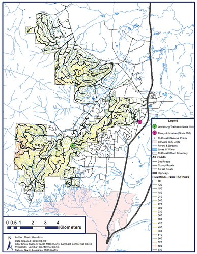
The McDonald Dunn Research Forest, Figure 2, is located to the north of Corvallis, Oregon and is managed by Oregon State University’s College of Forestry. The forest is over 4700 ha (47 km²) in size and the GIS database containing the harvest unit polygon and road line data has been under development starting in the 1980s and has been used for forest management since the late 1990s (Marshall et al. 1997). The surrounding highway and road networks have been included to access harvest units with landings inaccessible to the road network inside the forest. Velocity for each road segment is equal to the minimum of the speed limit for the road designation (e.g. minimum of stopping sight distance, maximum kW rate for regeneration system on steep grades). Velocity along each edge is assumed constant and velocity changes between edges, stops at intersections, and stops in turnouts were not included.

Figure 2. The McDonald Dunn research forest road networks, elevation contours, hauling origins and destinations.

Remotely sensed data acquisition and trimming

The LiDAR data used to derive the DEM was acquired from an airborne platform in 2000 (Hudak et al. 2002). The elevation of the study area based on the DEM ranges from 58 to 650 m and has an accuracy of 75 cm (horizontal) and 30 cm (vertical). The DEM was also trimmed to remove segments outside the study area.

Before analysis, this harvest unit polygon data was trimmed to improve visualization and split if a polygon could access multiple-harvest landings. Road line data were split at intersections, harvest landings, and major changes in road slope using the DEM data. Those split locations along with the end point of each road line were saved as node points.

Every node point was assigned an elevation value by overlaying the DEM raster. Next an attribute of the nearest harvest landing was assigned to each harvest polygon. New road length attributes were calculated based on the trimmed files and rolling resistance coefficient values were assigned to each segment. The rolling resistance coefficient attribute of normal force on paved surfaces was set to 0.013 kg/kg and 0.018 kg/kg on gravel based on estimates from the Logging Road Handbook (Byrne et al. 1960).

Road segment trimming process

Since energy expenditure and recovery is a function of the distance and the elevation change, an important part of the processing of the DEM data is the identification of road segments where regeneration of energy can take place (Liu et al. 2017). This road segment trimming added nodes identifying unique edges where energy regeneration is possible. Since the energy usage is nonconservative, even on edges where regeneration is possible, misidentification of regeneration segments and segment curvilinear lengths can underestimate energy needs.

For example, consider a 36,287 kg loaded truck is descending a minus 3% grade that is 305 m in length. If the coefficient of rolling resistance is 0.02 and air resistance is negligible then at 70% regeneration efficiency about 758.9 kJ could be put into the battery. However, if instead of a constant minus 3% grade, the actual grade between the nodes was 152.5 m at 0% slope and 152.5 m at minus 6% slope and if the power transmission efficiency was 75% for the part of the segment at 0% and 70% regeneration efficiency for the part of the segment at minus 6% then about 72.7 kJ could be put into the battery over the 305 m, a 90% reduction.

Network edge weight formula

The edge weight formula (Eq. 3(3) $\mathrm{If}\mathit{\theta }\ge 0,\mathrm{then}$(3) –14) used to calculate energy expended or regenerated across a road segment is a modified version of the derivation used by Sessions and Lyons (2018) to accommodate vehicles with and without regenerative braking. The formula factors in air resistance (AR) (Eq. 11(11) $\mathrm{AR}=\mathit{\hspace{0.17em}}0.5989\ast \mathrm{Frontal}\mathrm{Area}\ast \mathrm{Velocit}{\mathrm{y}}^2\ast \mathrm{Edge}\mathrm{Length}$(11) ), rolling resistance (RR) (Eq. 12(12) $\mathrm{RR}=\mathrm{CF}\ast \mathrm{RRCoeff}.\ast \mathrm{Truck}\mathrm{Weight}\ast \cos \left(\mathit{\theta }\right)\ast \mathrm{Edge}\mathrm{Length}$(12) ) and gravitational resistance (GR) (Eq. 13(13) $\mathrm{GR}=\mathrm{CF}\ast \mathrm{Truck}\mathrm{Weight}\ast \sin \left(\mathit{\theta }\right)\ast \mathrm{Edge}\mathrm{Length}$(13) ) as a measure of joules along each road segment edge length in meters with an angle Theta (θ) in radians. The formula also accounts for the conversion factor (Eq. 14) between kilogram-force meters and joules. Vehicle velocity, meters per second, is exogenous to the model, based on stopping sight distance or regulation which is assumed constant along the entire edge. Vehicle weight is in kilograms, frontal area is in meters squared and power train and regenerative braking efficiencies are decimal percentages. Battery capacity is assumed adequate to store regenerated energy, both in total kWh and in terms of regeneration capacity, kW. The rolling resistance coefficient (RRCoeff.) is expressed as kg per kg.

The edge weight formula for energy expenditure along a road line segment is modified to accommodate vehicles without regenerative braking (Eq. 9(9) $\left(\mathit{\theta }<0\right)\mathrm{and}\left(\left|\mathrm{GR}\right|>\left(\mathrm{AR}+\mathrm{RR}\right)\right)\mathrm{and}\mathrm{Regen}\mathrm{Efficiency}=0,\text{break}\mathrm{then}:$(9) & 10(10) $\mathrm{Edge}\mathrm{Weight}=0$(10) ) as well as to accommodate conditions where battery capacity or battery regeneration rate is exceeded. Edge length is the curvilinear slope length distance between node points.

(3) $\mathrm{If}\mathit{\theta }\ge 0,\mathrm{then}$(3)

$\mathrm{Edge}\mathrm{weight}=\left(\mathrm{AR}+\mathrm{RR}+\mathrm{GR}\right)$/Power train efficiency (4)

(5) $\mathrm{If}\left(\mathit{\theta }<0\right)\mathrm{and}\left(\left|\mathrm{GR}\right|\le \left(\mathrm{AR}+\mathrm{RR}\right)\right),\mathrm{then}:$(5)

(6) $\mathrm{Edge}\mathrm{Weight}=\left(\mathit{AR}+\mathit{RR}-\left|\mathit{GR}\right|\right)/\mathrm{Power}\mathrm{train}\mathrm{efficiency}$(6)

(7) $\mathrm{If}\left(\mathit{\theta }<0\right)\mathrm{and}\left(\left|\mathrm{GR}\right|>\left(\mathrm{AR}+\mathrm{RR}\right)\right)\mathrm{and}\mathrm{Regen}\mathrm{Efficiency}>0,\text{break}\mathrm{then}:$(7)

(8) $\mathrm{Edge}\mathrm{Weight}=\mathit{\hspace{0.17em}}-1\ast \left(\left|\mathrm{GR}\right|-\mathrm{AR}-\mathrm{RR}\right)\ast \mathrm{Regen}\mathrm{Efficiency}$(8)

(9) $\left(\mathit{\theta }<0\right)\mathrm{and}\left(\left|\mathrm{GR}\right|>\left(\mathrm{AR}+\mathrm{RR}\right)\right)\mathrm{and}\mathrm{Regen}\mathrm{Efficiency}=0,\text{break}\mathrm{then}:$(9)

$\mathit{\hspace{0.17em}}$

(10) $\mathrm{Edge}\mathrm{Weight}=0$(10)

Where:

(11) $\mathrm{AR}=\mathit{\hspace{0.17em}}0.5989\ast \mathrm{Frontal}\mathrm{Area}\ast \mathrm{Velocit}{\mathrm{y}}^2\ast \mathrm{Edge}\mathrm{Length}$(11)

(12) $\mathrm{RR}=\mathrm{CF}\ast \mathrm{RRCoeff}.\ast \mathrm{Truck}\mathrm{Weight}\ast \cos \left(\mathit{\theta }\right)\ast \mathrm{Edge}\mathrm{Length}$(12)

(13) $\mathrm{GR}=\mathrm{CF}\ast \mathrm{Truck}\mathrm{Weight}\ast \sin \left(\mathit{\theta }\right)\ast \mathrm{Edge}\mathrm{Length}$(13)

(14) $\mathrm{CF}=\mathit{\hspace{0.17em}}9.801$(14)

Internal python workflow system

Multi-network generation

After loading input data (Figure 1), FEVER prompts the user to select the truck configuration for the unloaded and loaded truck. Next, using the point (node) and road (edge) information, FEVER creates an adjacency list of the network points and roads. With the network adjacency list built, the tool then calculates the slope for each adjacent edge using the road lengths and point elevations. For each of the unloaded and loaded truck configurations, the tool applies the edge weight calculation, assigns weight to each edge in the network and builds two separate networks.

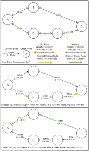
The tool builds two separate networks because vehicles with multiple routing options may not take the same route loaded as it did unloaded. For example, consider the network example for a chip truck in Figure 3 from nodes A to C, with a longer highway route and a shorter route on an unpaved road. This example shows that with all other inputs remaining constant, an unloaded chip truck with a power train and regenerative braking efficiency of 80% will require less energy to drive along the highway route compared an alternate route along the unpaved road route. In contrast, the same chip truck, with triple the gross weight in the same network, will require less energy to travel back along the alternate unpaved road. This illustrates that, with all other inputs remaining constant, an unloaded vehicle on a road network may take an alternative route to a loaded vehicle due to the energy gain from regenerative braking.

Figure 3. A multidirectional graph demonstrating the usage of alternate routes based on if a chip truck is loaded or unloaded. Routing is based on Figure 1 and edge weight energy calculations are based on Eq. 2(2) $\mathit{s}.\mathit{t}.\mathit{\hspace{0.17em}}\left(\mathrm{\forall e}\mathit{\hspace{0.17em}}=\mathit{\hspace{0.17em}}\left(\mathit{u},\mathit{\hspace{0.17em}}\mathit{v}\right)\mathit{\hspace{0.17em}}\in \mathit{\hspace{0.17em}}\mathit{E}\right),\mathit{\hspace{0.17em}}{x}_v\mathit{\hspace{0.17em}}\le \mathit{\hspace{0.17em}}{x}_u+\mathrm{\ell }\left(\mathit{e}\right),\mathit{\hspace{0.17em}}\mathit{xs}\mathit{\hspace{0.17em}}=\mathit{\hspace{0.17em}}0$(2) .

Navigation calculations

With the networks built, FEVER prompts the user to select a start location and destination. For every harvest polygon landing in the landscape, FEVER uses the Bellman-Ford (Ford 1956; Bellman 1958) routing algorithm to calculate the route with the lowest total energy cost from the start location along the unloaded network to the landing and then across the loaded network to the destination. Using this minimum energy route, the tool calculates and saves the total energy cost, travel time, and travel distance. These results are then assigned to each harvest landing node to be used later in the mapping module.

Mapping module

Once every harvest polygon has had its routing information calculated, the routing results are compiled and merged with the harvest unit polygons. FEVER then uses the merged results to create a routing result output table (Excel file) and initiates the mapping module. The mapping module plots the node points, road lines and harvest unit polygons. The mapping module colors the polygons based on total energy expenditure and energy expenditure as a function of road length.

Case study origin and destination selection

The start locations and destinations of this case study are the Lewisburg Trailhead and Peavy Arboretum. The Lewisburg Trailhead is in the center of the Southern half of the McDonald Dunn Research Forest and sits at mid elevation at 292 m. The Peavy Arboretum is on the Eastern edge of the McDonald Dunn Research Forest adjacent to Highway 99W. Both locations are common destinations for logging trucks transporting wood into and out of the forest. These locations were also chosen because they have multiple available routing options. Routing to each harvest unit was computed from each location back to that location and from each location to the other location.

Our study area was divided into 326 harvest landings (origins). For each origin, we construct a minimum energy route for the loaded vehicle to reach the specified destination and the minimum energy route for the unloaded vehicle to move from the destination and return to the origin. Thus, for each destination, our case study involved identifying 652 routes, 326 routes for the loaded vehicle and 326 routes for the unloaded vehicle,

Results

A summary of the harvest unit transportation energy costs and other travel data that the FEVER tool computes can be found in Table 2. The values in Table 2 are the combined average results from each start location node to every harvest polygon and then to the destination node. The tool also provides trip information for every shortest energy path from each start location node to every harvest polygon and then to the destination node.

Table 2. Routing summary data*.

Start Location Node	Destination Node	Avg Travel Cost (MJ)	Avg Travel Cost (KJ/km)	Min Travel Cost (MJ)	Max Travel Cost (MJ)	Avg Travel Time (Min)	Avg Travel Distance (Km)
101	101	162.5	8,953	0.1	349.0	25.4	19.0
190	190	135.0	6,151	1.2	269.7	25.2	20.8
101	190	96.4	4,222	−10.2	239.0	25.3	20.0
190	101	201.4	10,632	72	370.7	25.2	19.9

*Combined average results from each start location node to every harvest polygon and then to the destination node. Min and Max travel costs are the lowest and highest cost single trip and can be used to identify the maximum energy requirement to service an area.

The results of the mapping module have been output as shapefiles. Figures 4 through 7 show total megajoules to reach and return from each harvest unit. Similarly, Figures 8 and 9 show total energy cost normalized across the travel distance (kilojoules/km). Figure 10 shows road segment usage for the routing across the landscape. Additional examples of energy usage and road segment usage are in Appendix 2.

Figure 4. Harvest polygons colored based on total transportation cost (megajoules) for an empty R-500 - tandem traveling from the Lewisburg Trailhead (node 101) to the harvest polygon and then traveling back loaded to the Lewisburg Trailhead (node 101).

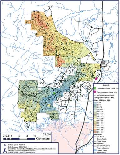
Figure 5. Harvest polygons colored based on total transportation cost (megajoules) for an empty R-500 - tandem traveling from the Peavy Arboretum (node 190) to the harvest polygon and then traveling back loaded to the Peavy Arboretum (node 190).

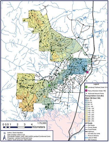
Figure 6. Harvest polygons colored based on total transportation cost (megajoules) for an empty R-500 - tandem traveling from the Lewisburg Trailhead (node 101) to the harvest polygon and then traveling back loaded to the Peavy Arboretum (node 190).

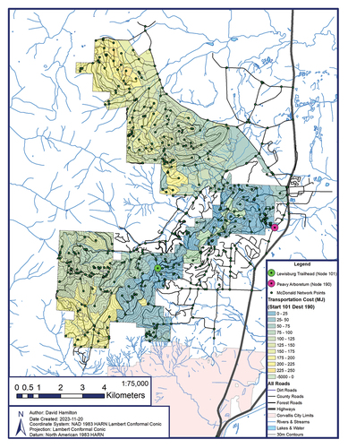
Figure 7. Harvest polygons colored based on total transportation cost (megajoules) for an empty R-500 - tandem traveling from the Peavy Arboretum (node 190) to the harvest polygon and then traveling back loaded to the Lewisburg Trailhead (node 101).

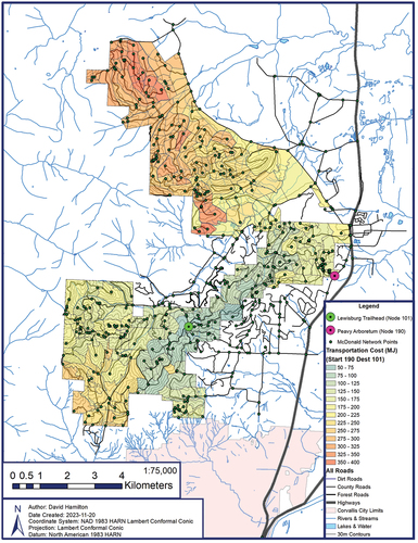
Figure 8. Harvest polygons colored based on total transportation cost as a function of distance (Kj/km) for an empty R-500 - tandem traveling from the Lewisburg Trailhead (node 101) to the harvest polygon and then traveling back loaded to the Lewisburg Trailhead (node 101).

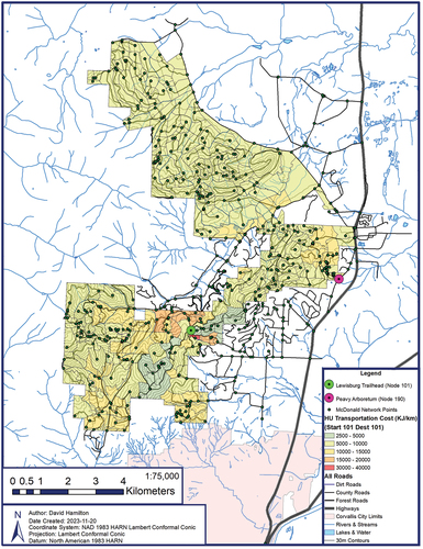
Figure 9. Harvest polygons colored based on total transportation cost as a function of distance (Kj/km) for an empty R-500 - tandem traveling from the Peavy Arboretum (node 190) to the harvest polygon and then traveling back loaded to the Peavy Arboretum (node 190).

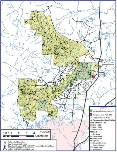
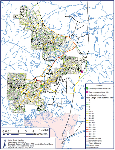
Figure 10. Forest roads colored based on the number of trucks that cross each road edge for every harvest landing on the trips from node 101 to node 101.

Discussion

Figure 4 shows that it requires considerably more energy to deliver logs from the low elevation harvest unit near Peavy Arboretum in the East, despite it being much closer to the Lewisburg Saddle. In Figure 5, the energy cost for transportation is much lower to southern harvest units which do not require a descent into the valley bottom to access, unlike the northern half of the forest. Figure 6 shows the cost of traveling from an empty point in mid elevation to a harvest unit and then delivering a load to low point and had an average travel cost of 96 MJ. Figure 6 also shows that at multiple points across the landscape a truck could regenerate more energy than it used. Figure 7 contrasts Figure 6 by traveling from an empty point in low elevation to a harvest unit and then delivering a load to a higher elevation averaging 201 MJ, a 108% increase in energy requirements compared to Figure 6 despite having an almost identical average distance and time.

Figures 8 and 9 show that the influence of regenerative braking on trip energy requirements has the greatest variation on short trips close to the origin/destination where grade changes are largest. Figures 8 and 9 also show that the average travel cost per meter experiences less variation between harvest units further from the origin and destination. This spatially illustrates that elevation and regenerative braking have less influence on average energy cost over longer distances where trucks are on lower gradient roads with less opportunity for regenerative braking. Also, as speed increases, the opportunities for regenerative braking are reduced due to the force to overcome air resistance increases as the square of the velocity.

Figure 10 shows the number of trips a truck takes over each given road segment for every routing option. Additional examples are in Appendix 2.

Conclusions

Forest operations planning applicability

FEVER allows analysts to spatially map the energy cost to access a forest landscape. The tool performs this function using a routing algorithm that differs from the tools currently available such as ESRI’s Network Analyst Tool (ESRI 2018) and Google Maps (Kim 2019). This case study spatially supports the findings of Sessions and Lyons (2018)s planning applicability. FEVER allows analysts to spatially map the energy cost to access a forest landscape. The tool performs this function using a routing algorithm that differs from the tools currently available such as ESRI’s Network Analyst Tool (ESRI 2018) and Google Maps (Kim 2019). This case study spatially supports the findings of Sessions and Lyons (2018) that regenerative braking can capitalize on elevation potential energy to deliver forest products to low elevation mills. FEVER can be used to help alleviate EV range anxiety by accurately mapping operational energy requirements, verify that new equipment can service a remote harvest site and be used to help perform forest scheduling.

Forestry GIS navigation system applications

One strength of FEVER is the ability to perform multiple iterations which identifies and tracks alternative routes based on changes in vehicle configuration such as weight or frontal area. This navigation tracking system allows forest operation planners to determine road usage at a glance and could be used to assist with hauling cycle timing, find unconventional routing options and allocate resources for road maintenance planning. FEVER can also save on maintenance fees by identifying redundant road segments that can be decommissioned.

Applications outside forestry and environmental impact

This system has applicability in any other industry that uses EVs with changing payloads such as mining, agriculture, and delivery services. These systems could employ FEVER to map quarries, farmland, and urban centers in the same manner to help planning efficient pickup and delivery routing. Globally heavy-duty trucks account for a disproportionately large share of emissions due to their high energy demand and reliance on diesel fuel. Within the United States, ICE vehicles are the largest contributors of fine particulate matter from transportation while also emitting a substantial amount of harmful NOx (EPA 2018). Heavy-duty vehicle electrification is necessary to reach the zero emission standards set out in the clean air act (State of California 2020). FEVER’s ability to map heavy-duty EV transportation costs can help combat climate change by assisting other industries striving to reach policy goals aimed at addressing emerging climate-related issues.

Patents

The FEVER tools, methodology, and subject matter of this paper are protected by United States Patent Application Number 18/349569. This paper serves as a practical guide for users interested in adopting the FEVER methodology.

Future work

The tool can be improved by adjusting the edge weight calculation to account for energy availability/expenditure to include battery storage capacity, battery regeneration rate, acceleration, current location, and incorporating the characteristics that account for the regenerative braking efficiency. Regenerative braking efficiency varies based on the type of storage, drive train efficiency, drive cycle and inertia weight (Clegg 1996). This data could be collected by adding a graphical user interface to the tool and mounting a GPS, accelerometer, and dynamometer into a test truck (Fajri et al. 2016). Finally, a sensitivity analysis (Saltelli 2002) could be conducted to identify the sensitivity of the energy estimation to a range of these variables, thereby identifying parameters that dominantly control the system and ranking those parameters.

The next step to improving this tool for industrial use would be to weight the edges based on transportation cost, which is usually a combination of unit distance cost and costs associated with working time. Having the tool to calculate total transportation cost across a landscape would be beneficial to major forest companies that own their own truck fleets because it can provide justification for switching to hybrid and electric systems by providing long-term estimated costs. Additionally, by including working, time planners and operators could perform maintenance scheduling and the tool could perform record keeping with respect to service intervals.

Another improvement to make FEVER more useful would be automating the trimming step in Figure 4. Developing a subroutine to automate the trimming along major slope changes and at intersections, harvest landings, destination points and the ends of roads would reduce the time it takes to build a forest network and improve usability by allowing users unfamiliar with GIS trimming processes to use the tool. This process could be taken a step further by adding a module to the tool that actively builds a GIS network as the machine is traveling by linking to a GPS. FEVER could then be linked to a cloud-based network so multiple trucks could build a database with their trip information with trips by different drivers yielding an appropriate hierarchical data structure (Liu et al. 2017). Daily trip-based energy consumption data collected over a long-term may remove variability in energy efficiency arising from unobservable variations in traffic conditions and driving habits.

Author contributions

Conceptualization, D.H.; methodology, D.H. and J.S.; software, D.H.; validation, D.H., and J.S.; formal analysis, D.H.; investigation, D.H.; resources, D.H.; data curation, D.H.; writing – original draft preparation, D.H. and V.D.; writing – review and editing, D.H., V.D. and JS.; visualization, D.H.; funding acquisition, J.S. All authors have read and agreed to the published version of the manuscript.

Geol¯ocation information

Acknowledgments: The authors acknowledge Edison Motors for providing truck specifications and developing the first hybrid electric logging truck; their groundbreaking vocational vehicle designs helped make this possible. The authors would also like to thank Molly Arnowil, John Sweet and all of OSU’s innovate team for their inspiration and support in the patent process.

Disclosure statement

No potential conflict of interest was reported by the author(s).

Supplementary Material

Supplemental data for this article can be accessed online at https://doi.org/10.1080/14942119.2024.2353501

Additional information

Funding

This research received no external funding. Work on this report received internal funding from Oregon State University’s Accelerator Innovation and Development fund.

References

- Abousleiman R, Rawashdeh, O. 2015. Energy consumption model of an electric vehicle. 2015 IEEE Transportation Electrification Conference and Expo (ITEC); Dearborn, MI, USA; 1–5. doi: 10.1109/ITEC.2015.7165773.
- Barber C, Little E. 2023. RSeries spec sheet: R500 & R750. [Internet]. [accessed 2023 Jun 5]. https://www.edisonmotors.ca/rseries.
- Bellman R. 1958. On a routing problem. Q Appl Math. 16(1):87–90. doi: 10.1090/qam/102435.
- Byrne JJ, Nelson RJ, Googins PH. 1960. Logging Road Handbook. Washington, DC: US Department of Agriculture.
- Clegg SJ. 1996. A review of regenerative braking systems. Leeds, UK: Institute of Transport Studies, University of Leeds. https://eprints.whiterose.ac.uk/2118/.
- de Nunzio G, Ojeda LL, Sciarretta A. 2022. Method of determining a route minimizing the energy consumption of a vehicle using a line graph. IEEE Control Syst. 35(5). doi: 10.1109/MCS.2015.2449688.
- Ding S, Li R. 2021. Forecasting the sales and stock of electric vehicles using a novel self-adaptive optimized grey model. Eng Appl Artif Intell. 100:104148. doi: 10.1016/j.engappai.2020.104148.
- [EPA] The Environmental Protection Agency. 2018. 2014 national emissions inventory report.
- [ESRI] Environmental Systems Research Institute. 2018. Algorithms used by the ArcGIS network analyst extension. ArcGIS desktop extensions [Internet]. [accessed 2023 Jun 8]. https://desktop.arcgis.com/en/arcmap/latest/extensions/network-analyst/algorithms-used-by-network-analyst.htm.
- Fagan S, Myers C. 2021. DEQ 17- clean air truck rules 2021 [Internet]. Salem: State of Oregon; [accessed 2023 May 28]. https://www.oregon.gov/deq/rulemaking/Pages/ctr2021.aspx.
- Fajri P, Lee S, Prabhala VAK, Ferdowsi M. 2016. Modeling and integration of electric vehicle regenerative and friction braking for motor/dynamometer test bench emulation. IEEE Trans Veh Technol. 65(6):4264–4273. doi: 10.1109/TVT.2015.2504363.
- Ford LR. 1956. Network Flow Theory. Santa Monica, California: RAND Corperation. https://www.rand.org/pubs/papers/P923.html.
- Forrest K, Mac Kinnon M, Tarroja B, Samuelsen S. 2020. Estimating the technical feasibility of fuel cell and battery electric vehicles for the medium and heavy duty sectors in California. Appl Energy. 276:115439. doi: 10.1016/j.apenergy.2020.115439.
- Grebner DL, Grace LA, Stuart W, Gilliland DP. 2005. A practical framework for evaluating hauling costs. Int J For Eng. 16(2):115–128. doi: 10.1080/14942119.2005.10702520.
- Hagberg AA, Schult DA, Swart PJ. 2008. Exploring network structure, Dynamics, and function using NetworkX. In: Varoquaux G, Vaught T Millman J editors. Proceedings of the 7th Python in Science Conference; Pasadena, CA USA: p. 11–15. https://www.osti.gov/biblio/960616.
- Harris CR, Millman KJ, der Walt SJ, Gommers R, Virtanen P, Cournapeau D, Wieser E, Taylor J, Berg S, Smith NJ, et al. 2020. Array programming with NumPy. Nature. 585(7825):357–362. doi: 10.1038/s41586-020-2649-2.
- Hudak AT, Lefsky MA, Cohen WB, Berterretche M. 2002. Integration of lidar and Landsat ETM+ data for estimating and mapping forest canopy height. Remote Sens Environ. 82(2–3):397–416. doi: 10.1016/S0034-4257(02)00056-1.
- Hunter JD. 2007. Matplotlib: a 2D graphics environment. Comput Sci Eng. 9(3):90–95. doi: 10.1109/MCSE.2007.55.
- Jordahl K, den Bossche J Van, Fleischmann M, Wasserman J, McBride J, Gerard J, Tratner J, Perry M, Badaracco AG, Farmer C, et al. 2020. Geopandas/geopandas: v0.8.1 [Internet]. 10.5281/zenodo.3946761.
- Kim YM. 2019. Dijkstra Algorithm: key to finding the shortest path, google map to Waze. Medium [Internet]. [accessed 2023 Jun 8]. https://medium.com/@yk392/dijkstra-algorithm-key-to-finding-the-shortest-path-google-map-to-waze-56ff3d9f92f0#:~:text=Google%20Map%20is%20based%20on,and%20pioneer%20in%20computing%20science.
- Konstantinou T, Gkritza K. 2023. Examining the barriers to electric truck adoption as a system: a grey-DEMATEL approach. Transp Res Interdiscip Perspect. 17:17. doi: 10.1016/j.trip.2022.100746.
- Liu K, Yamamoto T, Morikawa T. 2017. Impact of road gradient on energy consumption of electric vehicles. Transp Res D Transp Environ. 54:74–81. doi: 10.1016/j.trd.2017.05.005.
- Marshall DD, Johnson DL, Hann DW. 1997. A forest management information system for education, research and operations. Article J Forestry Washington. 95(10):27–30. https://www.researchgate.net/publication/258762599.
- McKinney W, and others. 2010. Data structures for statistical computing in python. In: Proceedings of the 9th Python in Science Conference July 10–16, 2023, Austin, Texas, p. 51–56. Vol. 445. and others.
- ODOT Commerce and Compliance Division. 2003. Oregon DoT: truck weight limits [Internet]. [place unknown];[accessed 2023 Jun 5]. https://www.oregon.gov/odot/MCT/Documents/weight_limits.pdf.
- Rezvani Z, Jansson J, Bodin J. 2015. Advances in consumer electric vehicle adoption research: a review and research agenda, transportation research part D. Transp Environ. 34(2015):122–136. doi: 10.1016/j.trd.2014.10.010.
- Saltelli A. 2002. Sensitivity analysis for importance assessment. Risk Anal. 22(3):579–590. doi: 10.1111/0272-4332.00040.
- Sessions J, Lyons CK. 2018. Harvesting elevation potential from mountain forests. Int J For Eng. 29(3):192–198. doi: 10.1080/14942119.2018.1527173.
- Sugihara C, Hardman S, Kurani K. 2023. Social, technological, and economic barriers to heavy-duty truck electrification. Sci Direct. 51(2023):101064–105395. doi: 10.1016/j.rtbm.2023.101064.
- State of California. 2020. Executive order N-79-20. Sacrimento, California: Executive Department.
- van Melkebeek D. 2004. CS 787: advanced algorithms: linear programming. University of Wisconsin Computer Science Department. [accessed 2023 Aug 11]. https://pages.cs.wisc.edu/~dieter/Courses/2004F-CS787/Scribes/lp.pdf.
- van Rossum G. 2020. The python library reference, release 3.8.2. [Internet]. [place unknown]: Python Software Foundation; [accessed 2023 Jul 3]. https://py.mit.edu/_static/spring21/library.pdf.