Quality ratings of frequency-compressed speech by participants with extensive high-frequency dead regions in the cochlea

Abstract

Objective: The objective was to assess the degradation of speech sound quality produced by frequency compression for listeners with extensive high-frequency dead regions (DRs). Design: Quality ratings were obtained using values of the starting frequency (Sf) of the frequency compression both below and above the estimated edge frequency, f_e, of each DR. Thus, the value of Sf often fell below the lowest value currently used in clinical practice. Several compression ratios were used for each value of Sf. Stimuli were sentences processed via a prototype hearing aid based on Phonak Exélia Art P. Study sample: Five participants (eight ears) with extensive high-frequency DRs were tested. Results: Reductions of sound-quality produced by frequency compression were small to moderate. Ratings decreased significantly with decreasing Sf and increasing CR. The mean ratings were lowest for the lowest Sf and highest CR. Ratings varied across participants, with one participant rating frequency compression lower than no frequency compression even when Sf was above f_e. Conclusions: Frequency compression degraded sound quality somewhat for this small group of participants with extensive high-frequency DRs. The degradation was greater for lower values of Sf relative to f_e, and for greater values of CR. Results varied across participants.

Key Words:

• Frequency compression
• dead regions
• hearing aids
• sound quality

View correction statement:

Erratum

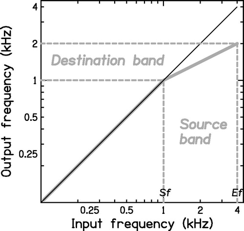
Frequency compression has been used as a method for conveying information carried by high frequencies to hearing-impaired listeners with high-frequency hearing loss (Simpson et al, 2005; Simpson et al, 2006; Glista et al, 2009; Bohnert et al, 2010; Wolfe et al, 2010, 2011; Park et al, 2012; Perreau et al, 2013; Hillock-Dunn et al, 2014; Hopkins et al, 2014; John et al, 2014; McCreery et al, 2014; Ellis & Munro, 2015; Kokx-Ryan et al, 2015; Wolfe et al, 2015; Alexander, 2014, 2016; Miller et al, 2016). When frequency compression is used, frequency components up to a “starting frequency” (Sf) remain unchanged in frequency and frequency components above Sf are shifted downwards by an amount that is proportional to the distance in octaves from Sf. The “amount” of frequency compression is specified by the frequency-compression ratio, CR. It is helpful to use the concepts of “source” and “destination” bands. The source band is the frequency band that is to be lowered. It has a low-frequency edge Sf and a high-frequency edge Ef. The width of the source band in octaves is 3.32 log₁₀(Ef/Sf). The destination band is the frequency band to which the source band is mapped. This band also has a low-frequency edge equal to Sf, while its width in octaves is 3.32 log₁₀(Ef/Sf)/CR. For example, if the source band extends from 1 to 4 kHz (2 octaves) and CR = 2, the destination band has a width of 1 octave and extends from 1 to 2 kHz. This is illustrated in Figure 1.

Figure 1. Input/output function for a frequency-compression hearing aid with Sf = 1 kHz and CR = 2. Frequency components below Sf remain unchanged. In this example, the high-frequency edge of the source band, Ef, is 4 kHz. The width of the source band in octaves is 3.32log₁₀(Ef/Sf), which is 2 octaves. The width of the destination band is 3.32log₁₀(Ef/Sf)/CR, which is 1 octave. Thus, its upper edge falls at 2 kHz.

Although studies evaluating the outcomes of frequency compression varied in several aspects (methods of fitting the frequency response and the settings of frequency compression, age and degree of hearing loss of the participants, study design, outcome measures), some of them demonstrated an advantage of frequency compression compared to conventional amplification for one or more measures of sound detection (Glista et al, 2009; Wolfe et al, 2010, 2011, 2015), plural recognition (Glista et al, 2009; Wolfe et al, 2010), identification of final /s/-/z/ in nonsense vowel-consonant syllables in noise. (Alexander, 2016), recognition threshold for some high-frequency sounds (Wolfe et al, 2010, 2015; Picou et al, 2015), recognition of at least some consonant sounds in quiet (Simpson et al, 2005; Hopkins et al, 2014; Ellis & Munro, 2015) and in noise (McCreery et al, 2014; Ellis & Munro, 2015; Alexander, 2016), and sentence intelligibility in noise (Bohnert et al, 2010; Wolfe et al, 2011; Ellis & Munro, 2015).

Audibility is an important factor in determining the outcomes of frequency compression (Alexander, 2013; Souza et al, 2013; Hopkins et al, 2014; McCreery et al, 2014). For people with severe to profound hearing loss, frequency-compression settings normally used in clinical practice often fail to provide adequate audibility (Hopkins et al, 2014). One reason for this is that Sf falls at frequencies where hearing thresholds are very elevated. Lowering the value of Sf would increase the chance of improving audibility but at the possible cost of poor sound quality. Poor sound quality could lead to withdrawal from hearing aid rehabilitation (Kochkin, 2000; Bertoli et al, 2009), so it is important to determine which settings of frequency compression are acceptable to hearing-impaired listeners.

Although sound quality was not directly addressed in most studies evaluating frequency compression [except for the studies of Souza et al (2013) and Picou et al (2015)], some studies provided anecdotal evidence of sound quality degradation for at least some participants. For example, four of seven participants tested by Simpson et al (2006) reported unacceptable sound quality when Sf was set to 1.25 kHz but not when Sf was increased to 1.6 kHz, and six of seven participants preferred the sound quality of the control hearing aid (with no frequency compression) over that of the frequency-compression hearing aid. Some subjects tested by Bohnert et al (2010), who used Sf values between 1.5 and 3 kHz, reported that fricative consonants sounded unnatural.

At the time of writing, there were seven studies of the effects of frequency compression on sound quality. One study assessed the sound quality of frequency-compressed music and not speech (Mussoi & Bentler, 2015). In three other studies, the effects of frequency compression on both speech and music were addressed (Parsa et al, 2013; Brennan et al, 2014; Picou et al, 2015). The remaining three studies were concerned with the effects of frequency compression on speech only (Souza et al, 2013; Johnson & Light, 2015; Miller et al, 2016). In three studies (Brennan et al, 2014; Picou et al, 2015; Miller et al, 2016), only one setting of frequency compression was used for each participant. That setting was selected to provide the greatest improvement in audibility while having the smallest impact on sound quality. Because the participants in these studies had mild to moderate hearing losses, only small amounts of frequency compression were used. Most of the participants tested by Brennan et al (2014) had Sf = 3.8 kHz and the average Sf of participants tested by Picou et al (2015) was 4 kHz. Such high values of Sf are unlikely to have a marked effect on sound quality. In the remaining three studies (Parsa et al, 2013; Souza et al, 2013; Johnson & Light, 2015), a range of frequency-compression settings [Sf = 2, 3, 4 kHz and CR = 2, and Sf = 3 kHz and CR = 6 and 10; Sf = 1.6, 2, 2.5, 3.15 kHz and CR = 2 for Parsa et al (2013); Sf = 1, 1.5 or 2 kHz and CR = 1.5, 2 or 3 for Souza et al (2013); and a range of individually chosen settings for Johnson and Light (2015)], as well as a control condition with no frequency compression were used, providing some insights into the effects of frequency-compression settings on sound quality.

For normal-hearing and at least for some hearing-impaired participants, the degradation in sound quality is greater for lower values of Sf and higher values of CR (Souza et al, 2013). This is likely to be related to the acoustical characteristics of speech. Low sound quality would be expected when Sf is set below the typical frequencies of the second formant of vowel sounds, which are below 1.5 kHz for most vowels produced by adult talkers (Peterson & Barney, 1952). The lower the value of Sf, the more vowel formants will be affected by frequency compression. The degradation of sound quality may also be partly a consequence of the inharmonicity produced by frequency compression; the upper partials in voiced speech sounds become “out of tune” with the lower harmonics.

Normal-hearing participants are more likely to report degraded sound quality than participants with hearing loss (Parsa et al, 2013; Souza et al, 2013). This may be the case because deficits in spectral analysis associated with hearing loss make the spectral changes associated with frequency compression less detectable. Consistent with this idea, Parsa et al (2013) found that while normal-hearing participants were able to distinguish between different settings of frequency compression (i.e. they gave them different ratings), hearing-impaired participants seem to be relatively insensitive to the distortion introduced by frequency compression for a high proportion of the settings used (i.e. they gave higher and more similar ratings across settings).

Another factor that may affect the sound quality of frequency-compressed speech is the balance between audibility and distortion. The increase in input frequency range made audible by frequency compression might lead to higher ratings while the distortion produced by frequency compression might lead to lower ratings. This could underlie the finding of Souza et al (2013) that participants with relatively poor hearing thresholds at 4, 6 and 8 kHz rated frequency-compressed speech as having equivalent quality to that for a control condition with no frequency compression, while participants with better hearing thresholds rated frequency-compressed speech as having lower sound quality than for the control condition. Consistent with this idea, for the participants tested by Brennan et al (2014) frequency-compressed speech and extended-bandwidth speech were equally preferred over restricted-bandwidth speech. Additionally, when a large amount of frequency compression is applied, the highest output frequency can be below the highest frequency that a given participant can hear with no frequency compression. This led to sound quality degradation for a group of participants tested by Johnson and Light (2015).

It is likely that, in practice, both the potential audibility benefit provided by frequency compression and the reduced sensitivity to distortion of hearing-impaired people play a role in the acceptability of frequency-compression settings for hearing-impaired participants. A suggested strategy for fitting frequency-compression hearing aids is to select frequency-compression parameters that improve audibility while minimising perceived distortion (Glista et al, 2009; McCreery et al, 2013; Brennan et al, 2014; Ellis & Munro, 2015; Picou et al, 2015; Miller et al, 2016). This has led to the choice of relatively high values of Sf (above 1.5 kHz) for hearing losses ranging from mild to severe.

At present, commercially available hearing aids use values of Sf of 1.5 kHz and above to avoid distorting the lower formants of speech. While this restriction is likely to be appropriate for many hearing-impaired people (Souza et al, 2013), people with more severe hearing loss may require lower values of Sf in order to increase the audibility of high frequencies. Moreover, some hearing-impaired participants may be more tolerant than others to lower values of Sf. This may apply particularly to people with extensive high-frequency dead regions (DRs) in the cochlea. These are regions with no or very few functioning inner hair cells, synapses, or neurons (Moore, 2001, 2004). The edge frequency of a DR is denoted f_e. People with extensive continuous DRs usually obtain limited benefit from amplification of frequencies above 1.7f_e (Vickers et al, 2001; Baer et al, 2002; Malicka et al, 2013). For such people, 1.7f_e is often below or near 1.5 kHz and therefore it might be desired to use values of Sf below 1.5 kHz. It is not known whether frequency compression adversely affects sound quality when Sf is below 1.5 kHz and Sf falls into a DR.

People with DRs have impaired pitch perception for tones whose frequencies fall within the DR, especially when the frequencies of the tones fall more than half an octave above f_e (Huss & Moore, 2005b). This might reduce their sensitivity to the inharmonicity produced by frequency compression, especially if the impaired pitch perception is related to reduced sensitivity to temporal fine structure (Moore, 2014). Also, frequency components falling above f_e, if sufficiently intense, are detected via the spread of basilar-membrane vibration to the place tuned to frequencies just below f_e; effectively, the frequency components are transposed in the cochlea. Therefore, it is not clear whether findings reported for participants with mild or moderate hearing loss without DRs should be generalised to people with DRs. Based on the perceptual consequences of DRs, we hypothesised that the use of low values of Sf may produce only small degradations of sound quality for participants with extensive high-frequency DRs.

The aim of this study was to determine if frequency compression with low values of Sf combined with several values of CR degrades the sound quality of speech for people with high-frequency DRs, and to estimate the extent of any degradation. We hypothesised that frequency compression may not significantly degrade the sound quality of speech even when Sf is low if Sf falls into a DR.

Materials and methods

Participants

Five participants (eight ears) with post-lingual sensorineural steeply sloping hearing loss and DRs with f_e values in the range 0.8–1.4 kHz were tested. All had air-bone gaps in their audiograms ≤10 dB and all had normal tympanograms. None had fluctuating hearing loss. Participants were native speakers of British English and reported no speech and language disorders. Table 1 summarises the demographics of the participants. Only one participant (P7_L) had experience with frequency-compression hearing aids. This participant had recently acquired frequency-compression hearing aids (Phonak Naída) and the value of Sf had been set to 2.2 kHz. However, f_e was 1 kHz for the test ear and the stimuli used for P7_L were low-pass filtered at 1.7 kHz (see below). Thus, P7_L had no experience with frequency compression over the audible frequency range of the stimuli.

Table 1. Demographic data of the participants.

ID	Gender	Age	Duration of hearing loss	Aetiology	Hearing aid use	Hearing aid type
P1	Female	63	28 years	Unknown	27 years	Oticon Spirit 3 Power
P2	Male	72	25 years	Noise-induced	14 years	Oticon Spirit 3 Power
P3	Female	77	20 years	Probably genetic	No HA	N/A
P5	Female	76	13 years	Unknown	13 years	Oticon Spirit 3 Power
P7	Female	71	44 years	Unknown	24 years	Phonak Naída

The research was approved by the LREC East of England Ethics Committee. Written consent was obtained from all participants. Participants were paid for their participation and their travel expenses were reimbursed.

Basic hearing assessment

Pure-tone audiometry using the procedure recommended by the British Society of Audiology (2011) was performed with a Grason-Stadler 61 audiometer at octave and semi-octave frequencies between 0.125 and 8 kHz for air conduction and at octave frequencies from 0.25 to 4 kHz for bone conduction. Tympanometry using the procedure recommended by the British Society of Audiology (1992) was performed using a 256-Hz probe tone presented via a Grason-Stadler 28 tympanometer. A tympanogram was considered to be normal if middle-ear pressure was between −50 and 50 daPa and compliance was between 0.3 and 1.6 cc.

Characterising DRs

Both the threshold-equalising noise (TEN(HL)) test (Moore et al, 2004) and fast psychophysical tuning curves (PTCs) (Sek et al, 2005) were used to detect and characterise DRs. For both tests, participants sat in a soundproof booth. The TEN(HL) test involves measuring the threshold for a pure tone in quiet and in a threshold-equalising noise (TEN). “HL” indicates that the noise and tone levels are calibrated in dB HL. The TEN(HL) is designed to produce equal masked thresholds in dB HL for all frequencies from 0.5 to 4 kHz for normally hearing listeners (Moore et al, 2004). The test is designed to detect off-frequency listening (listening at a place on the basilar membrane that is not tuned to the signal frequency). When a tone produces maximum basilar-membrane vibration in a DR, little or no information is transmitted to the auditory nerve from the place of maximum vibration. However, vibration at a place adjacent to the DR may be detected. Because the vibration at this remote place is lower than at the place of maximum excitation, the TEN(HL) is very efficient at masking the tone. Hence, the level of the tone needs to be increased considerably for it to be detected in the presence of the TEN(HL). A DR is deemed to be present when the masked threshold of the tone in the TEN(HL) is at least 10 dB above the threshold in quiet and 10 dB above the TEN(HL) level/ERB_N, where ERB_N stands for the equivalent rectangular bandwidth of the auditory filter for young normally hearing participants at moderate levels (Glasberg & Moore, 1990).

The TEN(HL) test was carried out using a Philips compact disc player type 753, a GSI 61 audiometer and TDH 50P headphones. The test tones had semi-octave frequencies from 0.5 to 4 kHz. The TEN(HL) level was set at least 10 dB higher than the absolute threshold (referred to as the “recommended level”) at the test frequency (Moore, 2001, 2004) whenever possible. There were three possible outcomes: (1) DR found (positive): The masked threshold of the tone in the TEN(HL) was 10 dB or more above the absolute threshold and 10 dB or more above the TEN(HL) level; (2) No DR found (negative): The masked threshold of the tone in the TEN (HL) was 10 dB or more above the absolute threshold and less than 8 dB above the TEN(HL) level; (3) Inconclusive: The masked threshold was 8 dB above the TEN(HL) level or the recommended level could not be used so the masked threshold of the tone in the TEN(HL) was less than 10 dB above the absolute threshold. In inconclusive cases, where possible the test was repeated using a higher level of the TEN(HL) (Moore, 2004).

Fast PTCs (Sek et al, 2005) were also used to diagnose DRs and to estimate the value of f_e. They were obtained using personal computers with an external M-Audio Audiophile USB soundcard, an M-Audio Delta 44 soundcard or a LynxOne soundcard whose output was routed via a Mackie 1202-VLZ PRO mixing desk. The output of the soundcard was routed via an Aphex HeadPod 454 headphone amplifier to one earpiece of Sennheiser HD580 headphones. A sinusoidal signal fixed at frequency f_s was presented at 10 dB sensation level (SL), that is 10 dB above the measured absolute threshold. A noise masker was presented at the same time as the signal. The noise masker was swept in centre frequency and its level was smoothly increased when the participant indicated that the signal was audible and decreased when the participant indicated that it was not audible. This procedure tracks the level of the masker needed just to mask the signal as a function of the masker centre frequency, that is the PTC. When no DR is present, the PTC is V-shaped, and its tip lies close to f_s. When there is a DR at f_s, the tip of the PTC is shifted away from f_s, as the signal is detected using neurons tuned away from f_s (off-frequency listening).

Initially, the absolute threshold at f_s was determined using the adaptive two-interval two-alternative forced-choice procedure implemented in the fast PTC software (Sek & Moore, 2011). For measurement of PTCs, the signal was pulsed, each pulse lasting 500 ms (including 20-ms raised-cosine rise/fall times) and each inter-pulse gap lasting 200 ms. The bandwidth of the masker was selected to prevent the participants from using beats as a cue (Kluk & Moore, 2005). A bandwidth of 0.2f_s was used for values of f_s up to 1.5 kHz and a bandwidth of 0.32 kHz was used for values of f_s above that, as recommended by Sek et al (2005). The masker centre frequency was swept in 0.1-kHz steps every 500 ms from well below f_s to just above it (upward sweep) or vice versa (downward sweep). The rate of change of the masker level was 2 dB/s. Each PTC measurement took 3–5 minutes. When necessary, a low-pass filtered noise was presented together with the “main” masker to prevent the detection of simple difference tones, as recommended by Kluk and Moore (2005).The level of the noise in a 1-ERB_N-wide band centred just below the noise cut-off frequency was 40 dB below the signal level. This level was chosen based on previous knowledge about the level of simple difference tones (Plomp, 1965).

Initially, upward-sweep fast PTCs were obtained for several values of f_s, including at least one low frequency where the outcome of the TEN(HL) test was negative. This was done to verify that the participant was able to carry out the task; the fast PTCs were expected to have tips close to f_s in such cases. Next, the value of f_s was increased in one-octave steps or up to the highest value of f_s for which the 10 dB SL signal was comfortably loud. Once a shifted tip was obtained, an upward-sweep and a downward-sweep PTC were obtained for that f_s. The fast PTC software provides several methods for estimating the frequency at the tip of the PTC, termed the minimum masker frequency (MMF). The method used here was a four-point moving average, which has a high success rate in estimating the MMF (Myers & Malicka, 2014). Spline interpolation was used to estimate the masker levels at a selected set of masker frequencies, and the levels at each frequency were averaged across the two runs. The masker centre frequency corresponding to the lowest level of the masker in the final average was taken as the estimate of the MMF. A shift of 10% or more of the MMF from f_s was taken as a positive indication of a DR at f_s (Moore & Malicka, 2013). The value of the MMF in such cases was taken as the estimate of f_e.

Stimuli for quality judgments

Fitting of the hearing aids

The stimuli were recorded from Phonak Exélia Art P behind the ear (BTE) hearing aids, modified by Phonak for the present study. In the unmodified hearing aids and fitting software, the lowest value of Sf is 1.5 kHz and the value of CR is linked to the value of Sf. In the modified hearing aids, values of Sf as low as 0.6 kHz could be used. Also, the value of CR was programmable independently of the value of Sf. For the reference stimuli, the frequency compression was switched off. Regardless of whether frequency compression was used, the hearing aids incorporated a low-pass filter with a cut-off frequency approximately equal to 1.7f_e. Typically, the output of the hearing aid dropped by 40 to 50 dB over the range 1.7f_e to 2.4f_e, and then flattened off. The choice of the cut-off frequency was based on the results described in the introduction, showing that people with extensive continuous DRs usually do not benefit from amplification of frequencies above 1.7f_e.

Offline processing and recording of stimuli made it possible to present the participant with different conditions in an efficient way, and to switch conditions during testing without the participant being aware of it. Thus, the participants did not wear the hearing aids during the study, but instead listened to stimuli pre-recorded from the hearing aids and presented via headphones.

To prepare the stimuli, one of the test hearing aids was programmed to fit the hearing loss of each test ear. Gains were adjusted to match the targets prescribed by the CAMEQ2-HF (now called CAM2) method (Moore et al, 2010) for frequencies up to 1.7f_e as closely as possible. The amplitude–compression ratio was limited to 3, since the Phonak Exélia Art P hearing aids use fast-acting compression, and there is evidence that high amplitude–compression ratios have deleterious effects when fast-acting compression is used (Verschuure et al, 1994). In the version of the CAM2 software used, limitation of the amplitude–compression ratio was achieved by maintaining the recommended high-level gains and decreasing the low-level gains relative to those recommended with the unrestricted amplitude–compression ratio (Moore et al, 2010). This would have reduced the audibility of weak and medium-level sounds.¹

Insertion gains were measured using a Madsen Aurical real-ear measurement system with the aid mounted on a KEMAR dummy head in a sound-proof booth with sound-absorbing walls, floor and ceiling. KEMAR was placed in front of the Aurical loudspeaker at a distance of 90 cm, as specified in the Aurical user manual. The legs of the table supporting the equipment were covered with 10-cm thick sound-absorbing foam and the KEMAR torso was covered with a t-shirt and a woollen pullover to reduce sound reflections. Targets were calculated for sinusoids with diffuse-field levels of 50, 65 and 80 dB SPL, and these were verified using a sweep tone. The reference stimuli were prepared using no processing other than amplitude compression and low-pass filtering with a cut-off frequency of 1.7f_e (defined as the 3-dB point relative to the response obtained with broadband amplification, as measured using a 2 cm³ coupler). The measured insertion gain was within 3 dB of the targets for nearly all the frequencies measured, and within 5 dB in the remaining few cases. Frequency compression was implemented using several values of Sf (as close as possible to 0.75, 1 and 1.25 times f_e), and several values of CR (2, 3 and 4), and was followed by low-pass filtering at 1.7f_e. This gave nine sets of frequency-compressed stimuli for each participant.

Recordings of the stimuli

The output of the hearing aid fitted to each ear was recorded via KEMAR, which was placed in the sound-proof booth described above at 1 m from a Tannoy Precision 8D self-powered loudspeaker with an azimuth of 0°. Stimuli were 96 sentences from the Bench–Kowal–Bamford (BKB) sentence lists (Bench et al, 1979), 48 spoken by a female and 48 spoken by a male. The stimuli were played at an overall level of 65 dB SPL (as measured with a Lucas CEL-414 Precision Impulse Type I sound level meter at the position corresponding to the centre of KEMAR’s head). Recordings were made using a Samsung P510 laptop connected to an external M-Audio Audiophile USB soundcard. The “pa_wavplayrecord” function in MATLAB was used to play out the sound files and record the output of the hearing aid simultaneously. For each set of stimuli, a calibration sound was recorded so that the recorded stimuli could be reproduced at the level that the hearing aid would have achieved if it had been worn by the participant during the test. Corrections were applied to compensate for the frequency response of the headphone used, so that the stimuli at the eardrum of the participant corresponded to those at the microphone in KEMAR’s ear canal.

After the recordings were obtained, the stimuli were high-pass filtered at 60 Hz to reduce any electrical noise that was present at 50 Hz. The filter was designed using the FIR1 function of MATLAB. It had 1103 coefficients and provided an attenuation of 12 dB at 50 Hz.

Procedure

A paired-comparison task was used. One sound within the pair was one of the reference stimuli and the other was frequency compressed with one of the combinations of Sf and CR, giving nine experimental conditions. Additionally, three blocks of trials were presented using no frequency compression, in which case the two sentences were identical. We refer to this as the control condition; the outcomes for these blocks were used to quantify the repeatability of the responses for each participant. Participants sat in a sound-proof booth for testing. Stimuli were presented via an M-Audio Delta soundcard hosted in a PC, and an Aphex HeadPod^TM 454 headphone amplifier connected to one earpiece of Sennheiser HD580 headphones. P5 suffered from claustrophobia and she was tested in a different booth with the door left open. Care was taken that the adjoining room was quiet. Stimuli were delivered to her via a Lynx One soundcard hosted in a PC via a Mackie 1202-VLZ PRO mixing desk.

Participants were required to indicate which sound of each pair was better in quality, and by how much, using a mouse-controlled slider on a computer screen (Füllgrabe et al, 2010), where zero indicated no difference, “−3” indicated “sentence one much better than sentence two”, and “3” indicated “sentence two much better than sentence one”. The scale was continuous. Participants could repeat the pair of sentences if needed. Instructions were: “You will hear a pair of sentences. Your task is to select the one you prefer in terms of sound quality and by how much. You can also indicate that the two sentences have the same quality if you think so”. Participants rated one training set containing two examples of each condition (in a random order) before starting the test.

Conditions were tested in a random order for each participant, with a complete block of trials for a given condition before moving to the next. To compensate for order effects within a block, for each participant and condition the reference stimulus was presented first in half of the trials and the frequency-compressed stimulus was presented first in the remainder. When ratings for each experimental condition were calculated, a negative sign was assigned to the nominal rating if the reference stimulus was preferred and a positive sign was assigned if the frequency-compressed stimulus was preferred. Each condition was assessed using twelve pairs of sentences, six spoken by the male talker and six spoken by the female. For half the ears, the test was performed first for the male talker and then for the female talker. The remaining ears were tested in the reverse order. Training and testing were carried out in a single two-hour session, including breaks. Short breaks were taken between blocks of trials as required, and a longer break between talkers was given.

Audibility calculations

The output of each hearing aid when mounted on KEMAR was measured using the “speechmap” function of an Interacoustics Affinity real-ear measurement system, for all conditions. KEMAR was placed in a sound-proof booth, at 55 cm from an Avantone Mixcube loudspeaker connected to the Affinity system. The output level in one-third-octave bands was compared with the hearing thresholds of the test ear to assess audibility as a function of frequency for each condition. The input was a 65-dB SPL speech-shaped noise whose spectrum matched the long-term average speech spectrum described by Moore et al (2008). Software provided by Phonak was used to calculate the input frequency for a given output frequency, so that the effective audibility for each input frequency could be calculated.

Results

Basic hearing assessment and characterisation of DRs

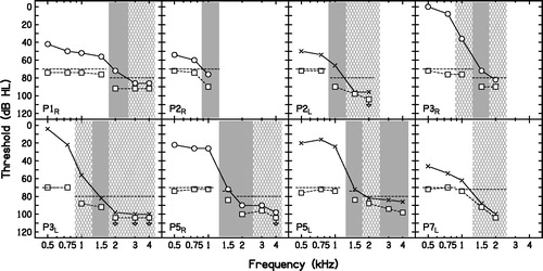
Figure 2 shows the air-conduction audiograms of the test ears. All participants had steeply sloping hearing loss. Figure 3 shows the results of the TEN(HL) test for the highest level of the TEN(HL) used in each case. As the maximum output level of the test tone was 104 dB HL, whenever the absolute threshold was close to or higher than this, the test could not be performed (see results for P2_R, at 1.5, 2, 3 and 4 kHz, P2_L and P3_R, and P7_L at 3 and 4 kHz). Inconclusive results were obtained for P1_R at 3 and 4 kHz; P2_L at 1.5 and 2 kHz; P3_R at 2 kHz; P5_R at 3 and 4 kHz, and P7_L, as the level of TEN(HL) was below the recommended level. Sometimes, even though the level of the TEN(HL) was either at or below the absolute threshold at the test frequency, a positive result was obtained (see results for P2_R at 1 kHz and P5_R at 1.5 and 2 kHz).

Figure 2. Air-conduction audiograms of the ears tested. Open circles and crosses indicate thresholds for the right and left ears, respectively. Down-pointing arrows indicate that the participant did not respond at the highest level tested.

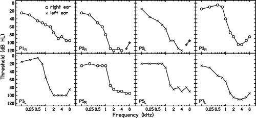
Figure 3. TEN(HL) test results. Audiometric thresholds measured as part of this test are shown using the same symbols as for Figure 2. When the audiometric threshold was higher than the maximum tone level of 104 dB HL, the threshold is not shown. The level of the TEN(HL) in dB/ERB_N is shown by the dashed lines without symbols. The masked thresholds of the tone in the TEN(HL) are shown by open squares. Downward-pointing arrows mean that the participant did not detect the tone at the level indicated. Shaded areas indicate frequencies where the outcome of the test was positive. Cross-hatched areas indicate frequencies where the outcome was inconclusive.

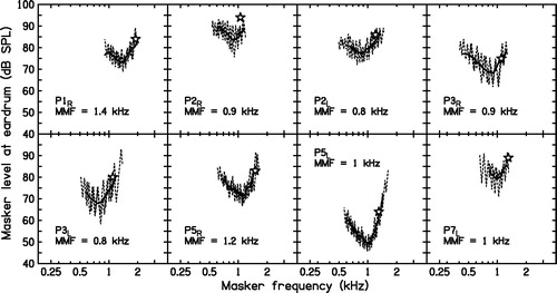
Figure 4 shows examples of the fast PTCs. The MMF was always below the lowest frequency that led to a positive result in the TEN(HL) test. In all cases, the MMF fell below f_s. This is indicative of high-frequency DRs.

Figure 4. Examples of PTCs. The signal frequency and level are denoted by an open star. The dotted line shows the masker levels visited, and the continuous line shows the combination of an upward-sweep and a downward-sweep run, after smoothing each of them. The frequency at the tip of each PTC (the MMF) is indicated in each panel. The MMF was taken as the estimate of f_e.

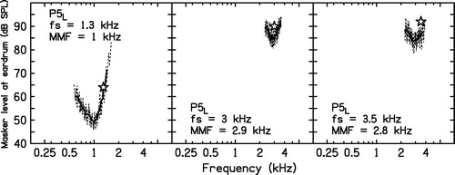
One case, P5_L, requires special attention, since the values of the MMF differed across signal frequencies. Additional PTCs for P5_L are plotted in Figure 5. For f_s = 1.3 kHz, the MMF fell close to 1 kHz, suggesting a DR starting at 1 kHz. An attempt was made to obtain a fast PTC for f_s = 2 kHz. However, for a signal level of 92 dB SPL, the masker level reached the maximum possible value shortly after the beginning of the test. It was not possible to mask the signal using the maximum masker level available from the equipment. Fast PTCs for higher values of f_s could be obtained without increasing the maximum level of the noise. For f_s = 3 kHz, the MMF was slightly shifted to 2.9 kHz. The shift is much less than 10% of f_s and it is not enough to diagnose a DR, although the TEN(HL) test outcome was positive for this frequency. For f_s = 3.5 kHz, the MMF was 2.8 kHz. This suggests a DR at 3.5 kHz, with a lower-frequency limit of 2.8 kHz. The most plausible interpretation of these results is that this participant had a restricted DR starting at about 1 kHz and ending below 2 kHz, and had another DR extending upwards from 2.8 kHz. There was probably a “island” of functioning inner hair cells and neurons starting just below 2 kHz and extending up to about 2.8 kHz.

Figure 5. Fast PTCs for P5_L. For f_s = 1.3 kHz, the tip was shifted to 1 kHz. For f_s = 3  and 3.5 kHz, the tips were shifted to 2.9 and 2.8 kHz, respectively. See the text for a discussion of these results.

The values of f_e for each ear were taken as the MMF values shown in Figure 4. Values of f_e ranged from 0.8 to 1.4 kHz.

Quality ratings

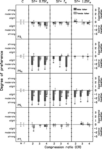
Figures 6 and 7 show the mean quality ratings for each ear and each condition. Mean ratings were mostly between −1 and about zero (where −1 meant “slight preference for the reference stimuli”). This means that, overall, frequency compression degraded sound quality, but the degradations were usually small. The error bars are described below. The mean ratings obtained from some ears (P1_R, P5_R, P5_L) were below −1, suggesting that frequency compression produced moderate degradation of sound quality for some conditions. For these ears, there was a trend for the ratings to decrease with decreasing Sf and increasing CR.

Figure 6. Mean quality ratings for P1_R, P2_R, P2_L and P3_R for each frequency-compression condition and for the control condition (C), plotted separately for each talker. Values of Sf and CR are shown at the top and bottom, respectively. Each row represents one ear. The error bars represent ±1 SD of the ratings after correction for order effects. For each ear, the leftmost panel shows the mean corrected ratings for the control condition when the reference stimulus was compared with itself, for the male talker (M) and the female talker (F). 95% confidence intervals were calculated from these ratings. Stars indicate that the mean ratings for a given frequency-compression condition were outside the 95% confidence intervals for the control condition.

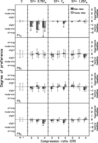
Figure 7. As Figure 6, but for P3_L, P5_R, P5_L and P7_L.

Group ratings

To assess the effect of frequency compression on sound-quality ratings at the group level, a within-subjects analysis of variance (ANOVA) was conducted with factors talker, Sf and CR, excluding the data for the control condition. This showed no significant effect of talker (F(1,7) = 2.67, p = 0.15). There was a significant effect of Sf (F(2,14) = 9.02, p = 0.003). A post hoc test with Bonferroni correction revealed that quality was significantly lower for Sf = 0.75f_e than for Sf = 1.25f_e (p < 0.017). Other pairwise comparisons between values of Sf were not significant. The effect of CR was also significant (F(2,14) = 7.42, p = 0.006). A post hoc test showed that quality ratings were significantly higher for CR = 2 and 3 than for CR = 4 (p < 0.017). Other pairwise comparisons were not significant. Quality ratings were lowest when low values of Sf were paired with higher values of CR. However, the interaction between Sf and CR was not significant (F(4,28) = 0.57, p = 0.69).

Individual ratings

The variability in the scores was partly a result of inherent variability in the judgments and partly a result of biases for choosing either the first or the second sound in the pair as the better-quality sound. Because the reference stimulus was presented equally often in the first and second intervals, the bias effect should be cancelled in the mean ratings.

To remove the effect of the systematic bias from the estimated variability of the ratings, the following procedure was adopted. Recall that a negative sign was assigned to the nominal rating if the reference stimulus was preferred and a positive sign was assigned if the frequency-compressed stimulus was preferred. For each subject and condition there were three ratings with the reference stimulus first (j1, k1, l1) and three with the reference stimulus second (j2, k2, l2). The mean bias effect was calculated as

Then, the ratings were “corrected” by adding B to each rating obtained when the reference stimulus was first and subtracting B from each rating obtained when the reference stimulus was second. For the control condition, no sign was assigned based on order. Instead, B was calculated as the negative of the mean rating. The ratings for the control condition were then corrected by adding B to each rating. The mean values of B for the control condition across talkers were −0.01, 0.12, 0.01, −0.4, −0.65, −0.2, −0.09 and −0.11 for P1_R, P2_R, P2_L, P3_R, P3_L, P5_R, P5_L and P7_L, respectively. The B values for P3 suggest that she had a bias for choosing the second sound in the pair for the control condition. For the experimental conditions, the mean values of B across talkers were −0.09, 0.12, −0.10, −0.28, −0.37, −0.07, −0.13 and 0.11 for P1_R, P2_R, P2_L, P3_R, P3_L, P5_R, P5_L and P7_L, respectively. Again, the values of B for P3 suggested a bias for choosing the second sound in a pair, but the bias was smaller than for the control condition. All subsequent analyses were based on the corrected ratings. The error bars in Figures 6 and 7 show ±1 standard deviation (SD) of the corrected ratings.

The corrected ratings for the control condition were used to estimate the inherent variability of the judgments. For each ear, the 95% confidence interval around the mean was computed from the combined results for the three blocks of trials for the control condition (CR =1 for both stimuli in each trial). If the mean score obtained for a given frequency-compressed stimulus was outside this 95% confidence interval, the results for this stimulus were deemed to be significantly different from those for the reference stimulus. Such cases are indicated by stars in Figures 6 and 7. Significant differences occurred for some conditions for P1_R, P3_R, P3_L, P5_R, P5_L and P7_L. P1_R preferred the reference stimulus to all frequency-compressed stimuli with Sf below f_e for both talkers; P3_R and P3_L preferred the reference stimulus when Sf = 0.75f_e and CR = 4 for the male and the female talker, respectively; P5_R preferred the reference stimulus to all frequency-compressed stimuli with Sf below or at f_e when the male talker was used; and P5_L preferred the reference stimuli to any of the frequency-compressed stimuli when the male talker was used, and preferred the reference stimulus to any setting of frequency compression with Sf below f_e and to frequency compression with Sf at f_e and CR 3 and 4. P7_L preferred the reference stimuli when Sf was below f_e and CR was 2 only for the female talker.

The SDs of the mean ratings were large for some participants and conditions. For some participants, it appears that when the participant could not hear a difference between the frequency-compressed and reference stimuli, the participant set the slider more or less randomly in a range below and above zero. P2 provides an example of this. In other cases, the reference condition was preferred in all or in five of six trials, and the strength of the preference varied across trials. Some responses of P1 and P5 are consistent with this pattern.

Audibility

Since the effective dynamic range of speech extends from 15 dB above the root-mean-square (RMS) level to 15 dB below it (ANSI, 1997), if the RMS level, L_f, of speech in a one-third octave band at a given frequency, f, is above the hearing threshold at that frequency, Thr_f, by 15 dB or more, the full dynamic range is audible at that frequency. If L_f is in the range ±15 dB relative to Thr_f, the proportion of the dynamic range that is audible at frequency f, P_f, is (L_f − Thr_f+15)/30. If L_f is 15 dB or more below Thr_f, the speech is completely inaudible at that frequency.

The results of the audibility calculations are summarised in Tables 2 and 3. For the reference stimuli, the tables specify the frequency at which P_f was 0.5 (0-dB relative level point) and where P_f just reached 0 (−15-dB relative level point). For the frequency-compressed stimuli, the tables specify: (1) The frequency at the lower edge of the source and destination bands (equal to Sf) and the relative level at that frequency; (2) The frequencies at the upper edges of the source and destination bands at which P_f was 0.5 (0-dB relative level point) and where P_f just reached 0 (−15-dB relative level point). In some cases, the relative level did not reach 0 dB for any frequency within the destination band. In those cases, source and destination frequencies are given for the destination frequency where the relative level was –8 dB.

Table 2. Audibility calculations for P1_R–P3_R.

			Lower edge		Upper edge
					0-dB or −8 dB relative level			−15-dB relative level
P	Sf	CR	Freq at Sf (kHz)	Rel level at Sf (dB)	Source (kHz)	Destination (kHz)	Rel level (dB)	Source (kHz)	Destination (kHz)
P1R	N/A	1	N/A	N/A	1.71	1.71	0	2.45	2.45
	0.75fe	2	1.00	11	3.00	1.73	0	4.75	2.18
		3	1.00	10	3.55	1.52	0	4.74	1.68
		4	1.00	9	4.05	1.41	0	4.05	1.61
	fe	2	1.40	8	1.80	1.59	0	3.95	2.35
		3	1.40	9	2.33	1.66	0	5.06	2.15
		4	1.40	10	2.47	1.61	0	4.90	1.92
	1.25fe	2	1.80	–4	3.25	2.41	–8	3.51	2.52
		3	1.80	–4	3.48	2.24	–8	4.51	2.44
		4	1.80	–4	3.45	2.12	–8	3.87	2.18
P2R	N/A	1	N/A	N/A	0.86	0.86	0	1.42	1.42
	0.75fe	2	0.70	0	1.57	1.05	–8	2.10	1.21
		3	0.70	0	1.82	0.96	–8	2.35	1.05
		4	0.70	0	1.26	0.81	–8	2.11	0.92
	fe	2	0.90	–2	1.26	1.06	–8	1.54	1.18
		3	0.90	–3	1.43	1.05	–8	1.84	1.14
		4	0.90	–4	1.97	1.10	–8	2.09	1.11
	1.25fe	2	1.10	–9	−8 dB not reached	−8 dB not reached	not reached	1.33	1.21
		3	1.10	–10	−8 dB not reached	−8 dB not reached	not reached	1.47	1.21
		4	1.10	–11	−8 dB not reached	−8 dB not reached	not reached	1.30	1.14
P2L	N/A	1	N/A	N/A	1.00	1.00	0	1.44	1.44
	0.75fe	2	0.60	12	1.45	0.94	0	2.82	1.30
		3	0.60	12	1.92	0.88	0	3.48	1.08
		4	0.60	10	1.80	0.79	0	3.75	0.95
	fe	2	0.80	4	1.10	0.94	0	2.44	1.40
		3	0.80	4	1.34	0.95	0	2.54	1.18
		4	0.80	4	1.49	0.94	0	2.60	1.08
	1.25fe	2	1.00	0	1.35	1.16	–8	1.74	1.32
		3	1.00	0	1.56	1.14	–8	1.94	1.25
		4	1.00	–2	1.46	1.10	–8	2.55	1.26
P3R	N/A	1	N/A	N/A	1.44	1.44	0	1.76	1.76
	0.75fe	2	0.70	29	2.49	1.32	0	3.51	1.57
		3	0.70	29	2.57	1.08	0	3.47	1.19
		4	0.70	28	2.81	0.99	0	4.19	1.10
	fe	2	0.90	20	1.78	1.26	0	3.15	1.68
		3	0.90	18	2.50	1.26	0	4.00	1.48
		4	0.90	20	2.80	1.19	0	3.94	1.30
	1.25fe	2	1.10	16	1.58	1.32	0	2.37	1.61
		3	1.10	12	1.98	1.34	0	3.33	1.59
		4	1.10	12	2.05	1.28	0	3.61	1.48

Columns 1–3 show the ear identifier, the value of Sf (the frequency at the lower edge of the destination band) relative to f_e, and the CR. CR =1 indicates the control condition, with no frequency compression. “Relative level” refers to the aided 1/3-octave RMS level at the destination frequency relative to the absolute threshold for that ear and frequency, when the input signal was a speech-shaped noise with overall level of 65 dB SPL. The columns labelled “Lower edge” show the value of Sf in kHz and the relative level at Sf. The columns labelled “Upper edge” show the source and destination frequencies at which the relative level was 0 dB (or –8 dB when 0 dB was not reached) and –15 dB. N/A means not applicable.

Table 3. As Table 2 but for P3_L–P7_L.

			Lower edge		Upper edge
					0-dB or –8-dB relative level			–15-dB relative level
P	Sf	CR	Freq at Sf (kHz)	Rel level (dB)	Source (kHz)	Destination (kHz)	Rel level (dB)	Source (kHz)	Destination (kHz)
P3L	N/A	1	N/A	N/A	1.25	1.25	0	1.61	1.61
	0.75fe	2	0.60	27	1.89	1.06	0	3.07	1.36
		3	0.60	29	2.70	0.99	0	3.65	1.10
		4	0.60	28	1.90	0.80	0	3.17	0.91
	fe	2	0.80	13	1.46	1.08	0	2.74	1.48
		3	0.80	12	1.81	1.05	0	2.90	1.23
		4	0.80	11	1.90	1.05	0	2.98	1.11
	1.25fe	2	1.00	6	1.25	1.11	0	2.01	1.41
		3	1.00	6	1.26	1.08	0	3.24	1.48
		4	1.00	2	1.02	1.01	0	3.21	1.34
P5R	N/A	1	N/A	N/A	1.50	1.50	0	2.03	2.03
	0.75fe	2	0.9	25	1.99	1.34	0	3.74	1.84
		3	0.9	25	2.72	1.30	0	3.85	1.46
		4	0.9	25	2.95	1.21	0	3.93	1.30
	fe	2	1.20	13	1.45	1.32	0	3.43	2.03
		3	1.20	13	1.82	1.38	0	3.95	1.78
		4	1.20	15	2.09	1.38	0	3.11	1.52
	1.25fe	2	1.50	–6	1.64	1.57	–8	2.74	2.03
		3	1.50	–8	1.50	1.50	−8	3.40	1.97
		4	1.50	–7	2.01	1.61	–8	3.55	1.86
P5L	N/A	1	N/A	N/A	1.42	1.42	0	1.81	1.81
	0.75fe	2	0.80	17	1.88	1.23	0	2.90	1.52
		3	0.80	19	2.44	1.16	0	3.16	1.27
		4	0.80	18	2.81	1.10	0	3.74	1.18
	fe	2	1.00	20	1.56	1.25	0	3.46	1.86
		3	1.00	20	2.03	1.26	0	3.11	1.46
		4	1.00	19	2.41	1.25	0	4.04	1.42
	1.25fe	2	1.30	0	1.55	1.42	–8	2.19	1.55
		3	1.30	0	1.61	1.40	–8	2.61	1.55
		4	1.30	0	1.74	1.40	–8	2.66	1.46
P7L	N/A	1	N/A	N/A	0.82	0.82	0	1.50	1.50
	0.75fe	2	0.80	1	0.98	0.88	0	2.66	1.46
		3	0.80	1	1.08	0.88	0	2.44	1.16
		4	0.80	1	0.89	0.82	0	2.65	1.08
	fe	2	1.00	0	1.36	1.16	–8	1.85	1.36
		3	1.00	0	1.42	1.13	–8	2.73	1.34
		4	1.00	–3	1.44	1.10	–8	2.55	1.26
	1.25fe	2	1.30	–11	−8 dB not reached	−8 dB not reached	not reached	1.54	1.42
		3	1.30	–10	−8 dB not reached	−8 dB not reached	not reached	1.42	1.34
		4	1.30	–11	−8 dB not reached	−8 dB not reached	not reached	1.46	1.34

Generally, the frequency compression did increase the range of source frequencies that was audible relative to that for the reference stimuli, as intended. The audible range of source frequencies tended to decrease with increasing Sf. This is due to the steeply-sloping shape of the participant’s audiograms. The audible range of source frequencies tended to increase with increasing CR, but this did not happen consistently. For two ears, P2_R and P7_L, audibility was very low for most conditions. This could account for the fact that quality ratings for these ears did not vary much with Sf or CR.

Discussion

At the group level, there was a significant effect of Sf, quality ratings for Sf = 0.75f_e being significantly lower than for Sf = 1.25f_e, and a significant effect of CR, CR = 4 leading to significantly lower sound-quality ratings than CR = 2 and 3. This is consistent with previous findings that low Sf and high CR values are associated with greater distortion of the signal (Parsa et al, 2013; Souza et al, 2013) and that the value of Sf had a significant effect on quality ratings for listeners with normal hearing and with moderate (Souza et al, 2013) and moderate to severe (Parsa et al, 2013) high-frequency hearing loss. However, here, the values of Sf varied across participants, as the values were selected based on the value of f_e. Thus, in the present study, the effect of Sf should be considered in the context of the DRs of the participants. For Sf = 0.75f_e, part of the frequency-compressed sound was delivered into the functioning frequency region just below f_e and part was delivered into the DR. For Sf = f_e, all of the frequency-compressed sound was delivered into the DR, in the range between f_e and 1.7f_e. For Sf = 1.25f_e, all of the frequency-compressed sound was delivered well inside the DR, in the range between 1.25f_e and 1.7f_e. Tones falling well inside a DR often do not have a clear pitch and sometimes sound noise-like (Huss & Moore, 2005a,b). This could partly account for the effect of Sf on quality ratings found here, as quality degradation may be less noticeable when the frequency-lowered sounds are delivered within a DR.

Based on previous studies (Parsa et al, 2013; Souza et al, 2013), it might be expected that, in the present study, the lower the value of f_e the greater the degradation in sound quality, as the absolute value of Sf decreased with decreasing f_e. This was not the case. For example, P1_R, P5_R and P5_L, whose f_e values ranged from 1 to 1.4 kHz, gave lower average ratings for frequency-compressed speech than P2_R, P2_L, P3_R, P3_L and P7_L, whose f_e values ranged from 0.8 to 1 kHz. It is possible that differences in auditory abilities across participants underlie these trends. P2, P3 and P7 had more severe losses than P1 and P5 (see Table 3). Consistent with this idea, Souza et al (2013), reported that participants with greater high-frequency hearing losses rated frequency-compressed and non-compressed speech as equal in quality, while participants with smaller losses rated the frequency-compressed speech as lower in quality. The lower sound-quality degradations for the participants with poorer high-frequency hearing may also be partly a consequence of reduced audibility for the frequency-compressed sounds. For example, for P2_R and P7_L, audibility was low for most conditions.

Differences in audibility across participants may have contributed to the individual differences in sound-quality ratings. For example, P7_L and P5_L, who used the same settings of frequency compression, gave different sound-quality ratings; P7_L gave average ratings close to 0, showing no clear preference, while P5_L rated the stimuli with frequency compression lower than the reference stimuli. Audibility was markedly worse for P7_L than for P5_L (as shown in Table 3). However, some participants with similar patterns of audibility, such as P3_R and P5_L, gave different patterns of quality ratings, with P3_R giving ratings close to 0 for most conditions, and P5_L showing preference for the reference condition across most settings of frequency compression, even though the values of Sf used for P3_R were slightly below those used for P5_L. This suggests that factors other than audibility influenced the sound-quality ratings. These factors could be related to pitch perception deficits associated with hearing loss and DRs, which could make the inharmonicity produced by frequency compression less detectable. Additionally, the maximum output frequency at which the RMS level of speech intersected the hearing threshold for some frequency-compression conditions was often below the maximum frequency at which the RMS level of speech intersected the hearing threshold without frequency compression (see 0-dB relative level for the destination band in Table 3). A reduction of the audible bandwidth may occur with extreme settings of frequency compression, and this can adversely affect sound quality (Johnson & Light, 2015). The ability to detect changes in bandwidth may have varied across participants.

We expected frequency compression not to degrade sound quality significantly when the frequency-compressed sounds were delivered completely within the DR, since in that case all of the frequency-compressed sounds that were audible were effectively transposed in the auditory system and detected via a place in the cochlea tuned just below f_e. The results are consistent with this. When Sf was 1.25f_e, significant quality degradation occurred only for ear P5_L, which had a surviving “island” which was not dead, probably starting just below 2 kHz and extending up to about 2.8 kHz, based on the fast PTCs. The upper edge of the destination band for P5_L was 1.7 kHz. Possibly, some of the frequency-compressed components falling just below 1.7 kHz were detected via upward spread of excitation to the surviving island, and this led to the degradation in sound quality for P5_L. For the other ear of the same participant (P5_R), the ratings for Sf = 1.25f_e were close to zero (i.e. the sound quality degradation was small or zero). This is consistent with the results for the other ears tested, and is as expected since, for this ear, the DR seemed to be continuous. However, it should also be noted that the value of f_e was slightly higher for this ear (1.2 kHz) than for P5_L (1 kHz), and so Sf was higher for P5_R than for P5_L for each condition tested. Higher Sf values are expected to cause milder degradation in sound quality (Parsa et al, 2013; Souza et al, 2013).

Finally, although the interaction of Sf and CR with talker was not significant for the group, some participants did vary in their preferences across talkers. Specifically, P1 and P5 showed greater preference for the reference stimuli when the male talker was used. This may be a consequence of the lower formant frequencies of the male than of the female voice, although it is not possible to rule out other factors, such as differences in overall spectral shape.

Although sound quality was mostly not degraded for Sf = 1.25f_e, there are some potential drawbacks of using this relatively high value of Sf: (1) The destination frequency range, between 1.25f_e and 1.7f_e, is narrow. Thus, for a given source band, the value of CR has to be higher than for Sf = f_e or 0.75f_e. Increasing CR may lead to a decreased ability to discriminate spectral differences between frequency-compressed sounds; (2) Pitch perception is very poor for frequency components falling well within a DR (Huss & Moore, 2005b). This could decrease the advantage that participants get from audibility of the frequency-compressed sounds; (3) Audibility often decreases with increasing frequency. Thus, audibility at 1.25f_e and above may be worse than at lower frequencies, limiting any potential benefit of frequency compression. Values of Sf below f_e allow wider source ranges to be delivered to the destination range using relatively low values of CR. However, such low values of Sf are likely to degrade sound quality to some extent, as shown by our results for Sf = 0.75f_e. A compromise is to set Sf = f_e, which led to a degradation in sound quality only for P5_R and P5_L.

When designing hearing aids for people with extensive DRs, as tested here, it may be useful to try alternative approaches in future research. A device that applies frequency lowering only when the short-term spectrum of the input signal is dominated by high-frequency components (conditional lowering) may be helpful. Conditional frequency lowering has been used with both frequency compression (Posen et al, 1993; Gifford et al, 2007) and frequency transposition (Robinson et al, 2007, 2009). With conditional frequency lowering, the device can be set so that it only lowers the frequencies of consonants whose spectra are dominated by high frequencies, such as fricatives, affricates and stops, and not consonants whose spectra are dominated by low and medium frequencies, such as approximants and nasals, or vowels. This might reduce the degradation of sound quality when low values of Sf are selected.

One limitation of the present study is the small sample of participants. Recruiting participants with extensive DRs was difficult, as their overall prevalence among the hearing-impaired population is only about 3% (Pepler et al, 2014). It would be desirable to test more participants with extensive DRs to assess the extent of individual variability within this population. Another limitation is that speech intelligibility was not explored. Some quality degradation might be tolerated if it were associated with large benefits for intelligibility. However, the initial acceptance of hearing aids is strongly influenced by sound quality (Kochkin, 2000), so reasonable sound quality is important if any benefits for speech intelligibility are to be realised.

In summary, frequency compression produced moderate degradations of sound quality for a small group of listeners with extensive high-frequency DRs. Quality was significantly lower when Sf was below than when it was above f_e, and quality was significantly lower for CR = 4 than for CR = 2 and 3. Ratings varied across participants. Preference for the reference condition was shown for several settings of frequency compression only for three ears, and two ears did not show any difference in preference between the reference and experimental conditions. Low audibility of the frequency-compressed components most likely accounts for the lack of strong preferences in two cases. For the remaining cases, the frequency-compressed components should have been audible, particularly for conditions with Sf = 0.75f_e. The degradation of sound quality when Sf was low might limit the acceptability of frequency-compression hearing aids with low Sf as implemented here. These results should be interpreted with caution, given the small sample size and the variability of results across participants.

Abbreviations
B	=	measure of bias effect
CR	=	frequency-compression ratio
DR	=	dead region
Ef	=	high-frequency edge of source band
fe	=	estimated edge frequency of dead region
fs	=	frequency of signal used for measuring a psychophysical tuning curve
Lf	=	the level of speech in a one-third octave band centred at frequency f
MMF	=	minimum masker frequency
Pf	=	audible proportion of the dynamic range of speech at frequency f
PTC	=	psychophysical tuning curve
SD	=	standard deviation
Sf	=	starting frequency of frequency compression
TEN(HL)	=	threshold equalising noise calibrated in hearing level
Thrf	=	hearing threshold at frequency f

Declaration of interest

The authors report no conflicts of interest. The authors alone are responsible for the content and writing of this article.

Funding was received from Action on Hearing Loss, Phonak AG and the H.B. Allen Trust (M.S.C.), and the Medical Research Council, UK (T.B. and B.C.J.M.).

Acknowledgements

We are grateful to Michael Stone for insightful discussion, Brian Glasberg for advice on statistical analysis, and Karolina Kluk and Josephine Marriage for their comments on an earlier version of this manuscript. We also thank two reviewers for helpful comments. We thank Phonak for providing the prototype hearing aids used here, as well as for technical support.

Notes

¹A more recent version of the CAM2 software, called CAM2A (not used in this study) limits the amplitude compression ratio by keeping the recommended gain for medium-level sounds, thus increasing the gain for high-level sounds while only slightly decreasing the gain for low-level sounds (Moore & Sek, 2016).

References

- Alexander, J.M. 2013. Individual variability in recognition of frequency-lowered speech. Sem Hear, 34, 83–109.
- Alexander, J.M. 2016. Nonlinear frequency compression: Influence of start frequency and input bandwidth on consonant and vowel recognition. J Acoust Soc Am, 139, 938–957.
- Alexander, J.M., Kopun, J.G. & Stelmachowicz, P.G. 2014. Effects of frequency compression and frequency transposition on fricative and affricate perception in listeners with normal hearing and mild to moderate hearing loss. Ear Hear, 35, 519–532.
- ANSI. 1997. ANSI S3.5-1997. Methods for the Calculation of the Speech Intelligibility Index. New York: American National Standards Institute.
- Baer, T., Moore, B.C.J. & Kluk, K. 2002. Effects of lowpass filtering on the intelligibility of speech in noise for people with and without dead regions at high frequencies. J Acoust Soc Am, 112, 1133–1144.
- Bench, J., Kowal, A. & Bamford, J. 1979. The BKB (Bamford-Kowal-Bench) sentence lists for partially-hearing children. Br J Audiol, 13, 108–112.
- Bertoli, S., Staehelin, K., Zemp, E., Schindler, C., Bodmer, D., et al. 2009. Survey on hearing aid use and satisfaction in Switzerland and their determinants. Int J Audiol, 48, 183–195.
- Bohnert, A., Nyffeler, M. & Keilmann, A. 2010. Advantages of a non-linear frequency compression algorithm in noise. Eur Arch Otorhinolaryngol, 267, 1045–1053.
- Brennan, M.A., McCreery, R., Kopun, J., Hoover, B., Alexander, J., et al. 2014. Paired comparisons of nonlinear frequency compression, extended bandwidth, and restricted bandwidth hearing aid processing for children and adults with hearing loss. J Am Acad Audiol, 25, 983–998.
- British Society of Audiology. 1992. Recommended procedure for tympanometry. Br J Audiol, 26, 255–257.
- British Society of Audiology. 2011. Recommended procedure for pure-tone air conduction and bone conduction threshold audiometry with and without masking. Reading, UK: British Society of Audiology.
- Ellis, R.J. & Munro, K.J. 2015. Benefit from, and acclimatization to, frequency compression hearing aids in experienced adult hearing-aid users. Int J Audiol, 54, 37–47.
- Füllgrabe, C., Baer, T., Stone, M.A. & Moore, B.C.J. 2010. Preliminary evaluation of a method for fitting hearing aids with extended bandwidth. Int J Audiol, 49, 741–753.
- Gifford, R.H., Dorman, M.F., Spahr, A.J. & McKarns, S.A. 2007. Effect of digital frequency compression (DFC) on speech recognition in candidates for combined electric and acoustic stimulation (EAS). J Speech Lang Hear Res, 50, 1194–1202.
- Glasberg, B.R. & Moore, B.C.J. 1990. Derivation of auditory filter shapes from notched-noise data. Hear Res, 47, 103–138.
- Glista, D., Scollie, S., Bagatto, M., Seewald, R., Parsa, V., et al. 2009. Evaluation of nonlinear frequency compression: Clinical outcomes. Int J Audiol, 48, 632–644.
- Hillock-Dunn, A., Buss, E., Duncan, N., Roush, P.A. & Leibold, L. 2014. Effects of nonlinear frequency compression on speech identification in children with hearing loss. Ear Hear, 35, 353–365.
- Hopkins, K., Khanom, M., Dickinson, A.M. & Munro, K.J. 2014. Benefit from non-linear frequency compression hearing aids in a clinical setting: The effects of duration of experience and severity of high-frequency hearing loss. Int J Audiol, 53, 219–228.
- Huss, M. & Moore, B.C.J. 2005a. Dead regions and noisiness of pure tones. Int J Audiol, 44, 599–611.
- Huss, M. & Moore, B.C.J. 2005b. Dead regions and pitch perception. J Acoust Soc Am, 117, 3841–3852.
- John, A., Wolfe, J., Scollie, S., Schafer, E., Hudson, M., et al. 2014. Evaluation of wideband frequency responses and nonlinear frequency compression for children with cookie-bite audiometric configurations. J Am Acad Audiol, 25, 1022–1033.
- Johnson, E.E. & Light, K.C. 2015. A patient-centered, provided-facilitated approach to the refinement of nonlinear frequency compression parameters based on subjective preference rating of amplified sound quality. J Am Acad Audiol, 26, 689–702.
- Kluk, K. & Moore, B.C.J. 2005. Factors affecting psychophysical tuning curves for hearing-impaired subjects with high-frequency dead regions. Hear Res, 200, 115–131.
- Kochkin, S. 2000. MarkeTrak V: “Why my hearing aids are in the drawer”: The consumers’ perspective. Hear J, 53, 34–42.
- Kokx-Ryan, M., Cohen, J., Cord, M.T., Walden, T.C., Makashay, M.J., et al. 2015. Benefits of nonlinear frequency compression in adult hearing aid users. J Am Acad Audiol, 26, 838–855.
- Malicka, A.N., Munro, K.J., Baer, T., Baker, R.J. & Moore, B.C.J. 2013. The effect of low-pass filtering on identification of nonsense syllables in quiet by school-age children with and without cochlear dead regions. Ear Hear, 34, 458–469.
- McCreery, R., Alexander, J., Brennan, M., Hoover, B., Kopun, J., et al. 2014. The influence of audibility on speech recognition with nonlinear frequency compression for children and adults with hearing loss. Ear Hear, 35, 440–447.
- McCreery, R.W., Brennan, M.A., Hoover, B., Kopun, J. & Stelmachowicz, P.G. 2013. Maximizing audibility and speech recognition with nonlinear frequency compression by estimating audible bandwidth. Ear Hear, 34, e24–e27.
- Miller, C.W., Bates, E. & Brennan, M. 2016. The effect of frequency lowering on speech perception in noise with adult hearing-aid users. Int J Audiol, 55, 305–312.
- Moore, B.C.J. 2001. Dead regions in the cochlea: Diagnosis, perceptual consequences, and implications for the fitting of hearing aids. Trends Amplif, 5, 1–34.
- Moore, B.C.J. 2004. Dead regions in the cochlea: Conceptual foundations, diagnosis, and clinical applications. Ear Hear, 25, 98–116.
- Moore, B.C.J. 2014. Auditory Processing of Temporal Fine Structure: Effects of Age and Hearing Loss. Singapore: World Scientific.
- Moore, B.C.J., Glasberg, B.R. & Stone, M.A. 2004. New version of the TEN test with calibrations in dB HL. Ear Hear, 25, 478–487.
- Moore, B.C.J., Glasberg, B.R. & Stone, M.A. 2010. Development of a new method for deriving initial fittings for hearing aids with multi-channel compression: CAMEQ2-HF. Int J Audiol, 49, 216–227.
- Moore, B.C.J. & Malicka, A.N. 2013. Cochlear dead regions in adults and children: Diagnosis and clinical implications. Semin Hear, 34, 37–50.
- Moore, B.C.J. & Sek, A. 2016. Comparison of the CAM2A and NAL-NL2 hearing-aid fitting methods for participants with a wide range of hearing losses. Int J Audiol, 55, 93–100.
- Moore, B.C.J., Stone, M.A., Füllgrabe, C., Glasberg, B.R. & Puria, S. 2008. Spectro-temporal characteristics of speech at high frequencies, and the potential for restoration of audibility to people with mild-to-moderate hearing loss. Ear Hear, 29, 907–922.
- Mussoi, B.S.S. & Bentler, R.A. 2015. Impact of frequency compression on music perception. Int J Audiol, 54, 627–633.
- Myers, J. & Malicka, A.N. 2014. Clinical feasibility of fast psychophysical tuning curves evaluated using normally hearing adults: Success rate, range of tip shift, repeatability, and comparison of methods used for estimation of frequency at the tip. Int J Audiol, 53, 887–894.
- Park, L.R., Teagle, H.F., Buss, E., Roush, P.A. & Buchman, C.A. 2012. Effects of frequency compression hearing aids for unilaterally implanted children with acoustically amplified residual hearing in the nonimplanted ear. Ear Hear, 33, e1–e12.
- Parsa, V., Scollie, S., Glista, D. & Seelisch, A. 2013. Nonlinear frequency compression: Effects on sound quality ratings of speech and music. Trends Amplif, 17, 54–68.
- Pepler, A., Munro, K.J., Lewis, K. & Kluk, K. 2014. Prevalence of cochlear dead regions in new referrals and existing adult hearing aid users. Ear Hear, 35, e99–e109.
- Peterson, G.E., Barney, H.L. 1952. Control methods used in a study of the vowels. J Acoust Soc Am, 24, 175–184.
- Perreau, A.E., Bentler, R.A. & Tyler, R.S. 2013. The contribution of a frequency-compression hearing aid to contralateral cochlear implant performance. J Am Acad Audiol, 24, 105–120.
- Picou, E.M., Marcrum, S.C. & Ricketts, T.A. 2015. Evaluation of the effects of nonlinear frequency compression on speech recognition and sound quality for adults with mild to moderate hearing loss. Int J Audiol, 54, 162–169.
- Plomp, R. 1965. Detectability threshold for combination tones. J Acoust Soc Am, 37, 1110–1123.
- Posen, M.P., Reed, C.M. & Braida, L.D. 1993. Intelligibility of frequency-lowered speech produced by a channel vocoder. J Rehabil Res Dev, 30, 26–38.
- Robinson, J., Baer, T. & Moore, B.C.J. 2007. Using transposition to improve consonant discrimination and detection for listeners with severe high-frequency hearing loss. Int J Audiol, 46, 293–308.
- Robinson, J., Stainsby, T.H., Baer, T. & Moore, B.C.J. 2009. Evaluation of a frequency transposition algorithm using wearable hearing aids. Int J Audiol, 48, 384–393.
- Sek, A., Alcántara, J.I., Moore, B.C.J., Kluk, K. & Wicher, A. 2005. Development of a fast method for determining psychophysical tuning curves. Int J Audiol, 44, 408–420.
- Sek, A. & Moore, B.C.J. 2011. Implementation of a fast method for measuring psychophysical tuning curves. Int J Audiol, 50, 237–242.
- Simpson, A., Hersbach, A.A. & McDermott, H.J. 2005. Improvements in speech perception with an experimental nonlinear frequency compression hearing device. Int J Audiol, 44, 281–292.
- Simpson, A., Hersbach, A.A. & McDermott, H.J. 2006. Frequency-compression outcomes in listeners with steeply sloping audiograms. Int J Audiol, 45, 619–629.
- Souza, P., Arehart, K.H., Kates, J.M., Croghan, N.B. & Gehani, N. 2013. Exploring the limits of frequency lowering. J Speech Lang Hear Res, 56, 1349–1363.
- Verschuure, J., Prinsen, T.T. & Dreschler, W.A. 1994. The effects of syllabic compression and frequency shaping on speech intelligibility in hearing impaired people. Ear Hear, 15, 13–21.
- Vickers, D.A., Moore, B.C.J. & Baer, T. 2001. Effects of lowpass filtering on the intelligibility of speech in quiet for people with and without dead regions at high frequencies. J Acoust Soc Am, 110, 1164–1175.
- Wolfe, J., John, A., Schafer, E., Hudson, M., Boretzki, M., et al. 2015. Evaluation of wideband frequency responses and non-linear frequency compression for children with mild to moderate high-frequency hearing loss. Int J Audiol, 54, 170–181.
- Wolfe, J., John, A., Schafer, E., Nyffeler, M., Boretzki, M., et al. 2010. Evaluation of nonlinear frequency compression for school-age children with moderate to moderately severe hearing loss. J Am Acad Audiol, 21, 618–628.
- Wolfe, J., John, A., Schafer, E., Nyffeler, M., Boretzki, M., et al. 2011. Long-term effects of non-linear frequency compression for children with moderate hearing loss. Int J Audiol, 50, 396–404.