Accuracy of averaged auditory brainstem response amplitude and latency estimates

Abstract

Objective: The aims were to 1) establish which of the four algorithms for estimating residual noise level and signal-to-noise ratio (SNR) in auditory brainstem responses (ABRs) perform better in terms of post-average wave-V peak latency and amplitude errors and 2) determine whether SNR or noise floor is a better stop criterion where the outcome measure is peak latency or amplitude. Design: The performance of the algorithms was evaluated by numerical simulations using an ABR template combined with electroencephalographic (EEG) recordings obtained without sound stimulus. The suitability of a fixed SNR versus a fixed noise floor stop criterion was assessed when variations in the wave-V waveform shape reflecting inter-subject variation was introduced. Study sample: Over 100 hours of raw EEG noise was recorded from 17 adult subjects, under different conditions (e.g. sleep or movement). Results: ABR feature accuracy was similar for the four algorithms. However, it was shown that a fixed noise floor leads to higher ABR wave-V amplitude accuracy; conversely, a fixed SNR yields higher wave-V latency accuracy. Conclusion: Similar performance suggests the use of the less computationally complex algorithms. Different stop criteria are recommended if the ABR peak latency or the amplitude is the outcome measure of interest.

Key Words:

• Auditory brainstem response, signal quality estimators
• post-averaged noise estimators
• ABR latency and amplitude errors

Introduction

Auditory evoked potentials (AEPs) represent the summation of electrical activity from nerve cells from all levels of the auditory pathway, recorded on the surface of the scalp in response to auditory stimulation. Typically, AEPs are small relative to the electrical background noise floor, particularly in the case of auditory brainstem responses (ABRs), since the recording electrodes on the scalp are far away from the sources. Although it is not possible to separate the desired evoked potential from the noise, the evoked potential can, to some extent, be recovered by averaging. Since the noise can be assumed to be random with respect to the response to the auditory stimuli, averaging tends to reduce the noise power. The evoked potential is often assumed to repeat in a deterministic way each time a new stimulus is presented and averaging will therefore not affect its power. The usefulness and reliability of the so-called post-average waveform, however, depends on the residual noise that it still contains.

Noise in evoked potential recordings can come from encephalic sources (e.g. variations in brain activity due to a changing state of arousal) and non-encephalic sources (e.g. muscle/movement artefacts, eye blinks and electrical artefacts). The noise in ABR measurements is often described as being non-stationary (Elberling and Wahlgreen 1985; Don and Elberling 1994), i.e. its statistical properties (e.g. mean value, power/variance) vary over time. Nevertheless, it is still a common practice both in research studies and clinical measurements to stop an ABR recording when a fixed number of stimulus presentations or epochs has been made which, in a given experiment, results in recordings of varying quality across subjects and stimulus types.

In the present study, the reliability of peak amplitude and latency of post-averaged ABRs, for a family of signal-to-noise ratio (SNR) estimator methods, was investigated to determine their practical reliability. Secondly, and perhaps more importantly an investigation was made on the criteria to determine when to stop averaging for a given ABR recording, in terms of errors or uncertainty in the post-average ABR peak amplitude and latency values. These are determined by the residual noise floor and the signal-to-noise ratio (SNR) of the waveform. As the signal and the noise cannot be separated, the true noise content of the post-averaged waveform is not known, and estimation methods must be employed. The analysis was focussed on ABR wave V, the largest and most commonly used response component. The present study made use of simulations using a database of raw EEG recordings from multiple subjects made with a typical ABR electrode configuration without any auditory stimulus. The degree of non-encephalic and encephalic noise was varied by controlling the movements and state of arousal of the test subjects. A “template” ABR signal was then added to epochs of the noise and averaging and different SNR estimation methods were applied and compared. Using simulations was necessary, as the true ABR peak amplitude and latency values need to be known a priori, such that the error could be properly quantified and compared. This approach is based on the assumption that the evoked response is fully deterministic and stationary. In reality, the AEP itself is likely not perfectly stationary, although generally considered to be substantially more so in most subjects (given competent recordings and compliant subjects) than the background noise. The validity of this assumption, in turn, depends on the stimulus rate varying over the course of a recording, as it is known that increasing stimulus rate results in a decrease in wave-V latency (Don, Allen, and Starr 1977) and amplitude (Burkard and Hecox 1987), reflecting auditory adaptation. Any variability that might by design be introduced into the stimulus rate for a given ABR recording is typically small enough not to affect the stationarity of the wave-V amplitudes and latencies. Therefore, the assumptions used in the present simulations reasonably reflect real recording conditions, and the use of a model response serves to assure a truly stationary, deterministic – namely, a perfectly known – signal as “the” response, leaving variances among the treatments to depend uniquely on the noises themselves.

Both residual noise floor estimators and signal-to-noise-ratio¹ estimators were considered, prior to investigating stopping criteria. The SNR algorithms considered in this study all belong to a group of methods known as variance ratios, which estimate the ratio, F, between the variance (mean-square value) of the recorded signal (response), σx², and an estimate of the variance of the background noise, σ_n², where the over-bars denote the post-average value: (1)

In the present study, four different estimates of the variance ratio were considered: The single-point F-ratio, F_SP (Elberling and Don 1984), the multiple-point F-ratio, F_MP (Don and Elberling 1994; Stürzebecher, Cebulla, and Wernecke 2001), Wong and Bickford’s (1980) measure, F_WB (Wong and Bickford 1980) and the non-stationary multiple point F-ratio, NSF_MP (Silva 2009). A short mathematical description of some of these methods is provided in the appendix in the Supplementary material. Furthermore, this study explored the effect of the averaging stopping criteria (estimated SNR or post-average residual noise variance) on ABR wave-V amplitude and latency estimate accuracy. For this purpose, the width and amplitude of the ABR template were varied systematically to reflect across-subject differences and the accuracy of the latency and amplitude estimates was evaluated to determine whether a fixed noise variance or a fixed SNR is a good stop criterion. Such an analysis, with a focus on wave-V amplitude and latency accuracy, to the authors’ knowledge has not previously been considered in the literature.

Method

Auditory brainstem response in noise

A simple model of ABR generation was considered that assumes that each epoch recorded to individual stimuli, x(t), consists of the ABR signal, denoted here as s(t), and an additive random noise term η_k (t): (2) where k is the trial or epoch number. It is assumed that the underlying ABR, s(t), does not change with each trial, but remains fixed. In contrast, the noise is changed on a trial by trial basis. Using the matrix notation given in (Silva 2009) and (Davila and Mobin 1992), the ensemble of all trial data can be rewritten as: (3) where K is the total number of recorded trials included in the average, S(t), N (t) and X(t) are K × T matrices and T is the number of samples recorded in each trial.

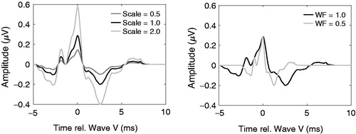
The template (model) used for the ABR within each trial could then be combined with EEG recorded under different test conditions reflecting different degrees of non-encephalic noise. If EEG recordings were made with an auditory stimulus, then there would be no a priori knowledge of the true amplitudes and latencies. The template ABR considered was obtained in (Elberling, Callø, and Don 2010) (see left panel of Figure 1 with scale factor of 1.0), by aligning the wave-V peaks across recordings from 10 young adults with normal hearing by conventional audiometry and negative neurologic histories and taking the inter-subject average computing the grand-average response across subjects. The stimulus was a 100 μs standard click presented via ER-2 insert earphones at 60 dB nHL (approx. 103.5 dB peak-to-peak sound pressure level, peSPL, (ISO 389–6 2007). The template ABR has a true wave-V amplitude of 0.488 μV. In the present study, the wave-V amplitude was calculated as the peak-to-through difference.

Figure 1. Templates used to represent the ABR signal. Scaled ABR templates (left panel) and ABR templates with reduced wave-V width (right panel).

EEG noise database

The background EEG activity was measured under four different test conditions: “sleep”, “still”, “blink” and “head movement” in order to collect a selection of noise with different levels and different proportions of non-encephalic noise. In the “sleep” condition, the subjects were instructed to “try to sleep” during the recordings; in the “still” condition, they were instructed to lie still with their eyes closed without sleeping; in the “blink” and “head movement” conditions, they were instructed to lie still and to blink or to move according to an animation shown on a monitor in the testing booth, respectively.

Measurements were carried out using a Compumedics SynAmps 2 EEG amplifier, in an electrically shielded and sound isolated double-walled booth. EEG noise was recorded with (Ag/AgCl) scalp electrodes (impedance < 5 kΩ) with the active electrode placed on the left mastoid, the ground on the right cheek and the reference on the high forehead, namely per electrode montage favoured for clinical recordings. A sampling frequency of 20 kHz was used and the raw EEG was filtered between 0.03 and 3 kHz using digital second order Butterworth filters (12dB/oct.). Each recorded run consisted of 10,000 epochs of 20 ms duration. However, a relatively stringent offline artefact rejection criterion of 20μV was used, thus the number of epochs per run were eventually less than 10,000, particularly for the movement conditions. Three runs were recorded for each subject for each of the “still”, “blink” and “head movement” conditions. In contrast, in the “sleep” condition seven runs were recorded for each subject. In this case, all recordings were included from subjects who self-reported that they had been sleeping, implying that the “sleep data” very likely included epochs where the subjects were awake and epochs where they were sleeping. This could not be avoided in the present study and the data could thus be considered to only represent a “relaxed” condition.

Noise was measured from 12 male and four female subjects between 24 and 32 years of age and one female subject of 52 years of age. Each subject volunteered for at least two of the test conditions. Audiometric thresholds were below 20 dB HL for all except one subject. The data from this subject were comparable to data from other subjects and were therefore included in the database. To ensure similar level of noise in each condition runs, outlying runs were removed using the Median rule (Carling 2000) according to the variance in each run. Between 3.1 and 6.4% of runs were removed from each condition resulting in the removal of a total of 9 out of 163 runs. The data remaining after outlier removal represented the database of EEG noise. A total of 44 runs from eight subjects was recorded for the sleep condition; 47 runs from 17 subjects for the still condition; 31 runs from 11 subjects for the blink condition and 32 runs from 11 subjects for the movement condition. All experiments were approved by the Science-Ethics Committee for the Capital Region of Denmark.

Block-weighted (Bayesian) averaging

The way in which the individual ABR epochs are averaged can have a significant impact on the residual noise floor (see for example [Elberling and Wahlgreen 1985; Lutkenhöner, Hoke, and Pantev 1985; Mühler and von Specht 1999; Riedel, Granzow, and B. Kollmeier 2001; Elberling and Don 2008). The present study only considered block-weighted (also known as Bayesian) averaging, where weights inversely proportional to an estimate of the background noise power are used to reduce the effects of non-stationarity in the noise.

Traditional averaging takes the mean of all K epochs in the recording, which is the same as summing and weighting each epoch by In contrast, weighted averaging reduces the effects of non-stationarity in the noise power by using weights that are inversely proportional to an estimate of the background noise power of each epoch (weighted averaging) or block of epochs (block-weighted averaging), such that epochs with a large noise power are penalised over those with a low noise power. In this study, block-weighted averaging was employed because the noise variance estimate has been shown to be more accurate when made from a block of epochs instead of a single epoch (Elberling et al. 2007). The post-averaged waveform can be written as: (4) where w is a K × 1 weight vector whose values are dependent on the type of averaging employed. The K trials were split into B blocks, each consisting of β epochs. In block-weighted averaging, the noise power is considered to be slowly varying and stationary across all epochs within a given block. Using the notation (Silva 2009), the weight vector is given by: (5) where ∧ R_η ^{- 1} is an estimate of the inverse K × K covariance matrix of the noise and - 1^T represents the vector [1 1 ⋯ 1 ]. The noise was assumed here to be a stationary zero-mean Gaussian white noise process within each block of trials (i.e. locally stationary). The covariance matrix is therefore diagonal with B blocks of repeated elements: (6) where R_η b = ,σ_η b²I. Thus, R_{η b} represents the diagonal covariance matrix for block b (out of a total of B blocks, each with β trials) and I denotes the identity matrix.

Each of the four algorithms investigated in this study uses a different method to obtain an estimate of the noise power, ∧ σ_η b², used in the weight estimate. Here, the symbol ‘^’ denotes an estimated quantity.

Numerical simulations

Numerical simulations were run to investigate the performance, via wave-V latency and amplitude estimation error, of different variance ratio algorithms and averaging stop criteria. The post-average waveform is affected by the noise variance estimate due to the use of block-weighted averaging. Wave-V amplitude, wave-V latency, SNR, and noise variance estimates were calculated for successively larger multiples of 32 epochs (block-size, β; a blocksize of 32 was used here as it was the minimum block size used in Silva (2009) of each recorded noise run combined with the ABR template. The data from many subjects and for several test conditions were included, reasonably expected to provide a good indication of the spread of results in typical ABR measurements, as well as providing latency and amplitude estimates for a wide range of variance ratios.

In the simulations, the post-averaged wave-V peak was found as the sample having the maximum amplitude within ±1 ms from the sample number of the true wave V. The latency was then estimated as the difference in time between this sample number and the beginning of the epoch. The amplitude was found, by similarly identifying the trough of wave V as the minimum within ±1 ms from the true trough and then calculating the difference between the amplitudes of the peak and trough, per convention.

For both the F_MP and NSF_MP algorithms, the noise variance was estimated across all epochs at seven fixed points (see appendix in Supplementary material for more information about the algorithms). The choice of a number of seven fixed points for epochs with duration of 20 ms was based on the findings in (Elberling and Don 1984) showing that the degree of freedom was five in the worst case for an epoch length of 15 ms and a sampling frequency of 20 kHz. This suggested that adjacent points need to be separated by at least 3 ms in order to be independent from each other.

Comparison of F-ratio methods

The variance ratios and post-average wave-V latency and amplitude estimates were calculated for each algorithm. The performance of the different algorithms was evaluated and compared for fixed variance ratios in terms of latency and amplitude estimate accuracy.

Averaging stop criteria

The accuracy of the wave-V latency and amplitude estimates was investigated for a fixed SNR or a fixed noise level for ABR waveforms of varying width or amplitude. Two sets of simulations were run. In the first simulation, the ABR template amplitude was varied by multiplying it with scale factors of 0.5, 1 and 2, respectively and the variance ratios, noise levels and wave-V latencies and amplitudes were calculated. In the second simulation, the width of the ABR waveform (via resampling the template) was scaled in time by a factor of 0.5 resulting in a sharper ABR wave-V peak. All modified ABR templates are shown in Figure 1.

Results

EEG Database

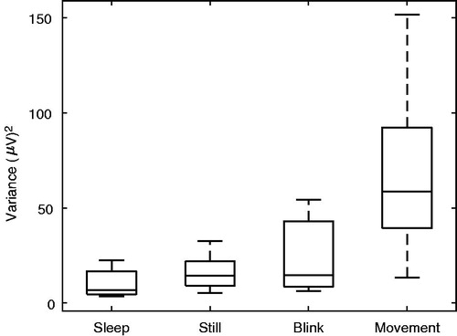
Figure 2 shows a box-and-whisker diagram to graphically represent the global (long-term) sample variance for each run within the database. The box shows the median (center line - second quartile) as well as the first and third quartiles. The whiskers are drawn from minimum to maximum after outliers have been removed. It can be seen that there are slight differences between the variances from the sleep, still and blink conditions. As expected, the greatest difference was observed between the variances from these three conditions and the movement condition. The database thus indeed contains runs with a variety of variances for each test condition. This provides a good basis for the test of the individual SNR algorithms.

Figure 2. The global variance of data of each run included in the database for each condition. No artefact rejection was applied here. Thus, this represents the raw data in the EEG noise database.

Comparison of F-ratio estimates

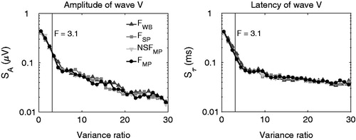
Figure 3 show the difference (error) between the estimated and true amplitudes (upper panels) and latencies (lower panels), respectively, as functions of the variance ratio for the F_MP (left panels) and the NSF_MP (right panels) algorithm, respectively. Here, for each run in the whole database (all four conditions), the number of averaged epochs was successively increased by 32 to obtain a spread of F-ratios, yielding the likely distribution of errors as a function of the F-ratio. In these scatter plots, each point represents one estimated amplitude error and the grey solid curves show the mean error, or bias, as a function of variance ratio.

Figure 3. Scatter plots showing the difference between the estimated and true amplitudes (∈_A) and latencies (∈_τ) of wave V as a function of variance ratio. The grey-lines show the mean error or bias, E[∈_A] and E[∈_tau]. The left and right hand figures show the cases for F_MP and NSF_MP, respectively. The errors for F_WB and F_SP are not shown for brevity.

It can be seen that the distributions of all of the points are very similar for the F_MP and NSF_MP methods. A similar result was found for the F_WB and F_SP (not shown for brevity). The vertical line in each panels shows an F-ratio of 3.1, which indicates with a 99% accuracy that a repeated response is present (based on an F-test with 5 and 250 degrees of freedom) in the residual post-averaged waveform (Elberling and Don 1984) and permits the assumption that the noise distribution is zero mean, Gaussian and stationary. The distributions of errors are all wider at low variance ratios and get narrower and tend towards zero with increasing variance ratio. This was expected since a relative higher noise level (i.e. low variance ratio) should result in a higher error than a lower-level noise level (high variance ratio).

The latency error scatter plots (lower panels) are also broader at low variance ratios and tend towards zero with increasing variance ratio. Indeed, for F-ratios above 3.1, the distribution is symmetrical around a latency error of zero. Below 3.1, the distribution is almost uniform verifying the recommendations for ABR recordings suggested by (Elberling and Don 1984). It can be seen that the error extends to ±1 ms which was the limit imposed on the automatic identification procedure. A pronounced feature in these latency scatter plots are their stratified nature which occurs due to the sampling interval (0.05 ms).

The latency and amplitude error distributions obtained with the different algorithms are very similar. The standard errors (i.e. the standard deviation of the error estimates for amplitude (S_A) and latency² (S_τ) representing the spread of errors for each variance ratio were considered here as a metric to compare the distribution of errors for the different algorithms. To ensure sufficient numbers of values for each standard error calculated, error values were grouped based on variance ratio intervals of 1. The standard errors obtained for the amplitude and latency estimates are shown in Figure 4. It can be seen that the standard deviation decreases with increasing variance ratio. It is clear that there is little variation among the errors obtained with the different algorithms. Thus, this metric of performance only reveals very small difference among the four algorithms.

Figure 4. Standard error of wave-V amplitude estimates for fixed variance ratio intervals (left panel). Standard deviation of wave-V latency estimates for fixed variance ratio intervals (right panel).

Averaging stop criteria

Figure 5 shows the standard deviation of wave-V amplitude (S_A; upper panels) and latency (S_τ; lower panels) errors as a function of the fixed F_MP. The resulting ABRs had wave-V amplitudes ranging from 0.244 to 0.976 µV. For comparison, Elberling, Callø, and Don (2010) measured wave-V amplitudes (±2 SD from the mean) for a 60 dB nHL standardised click ranged from 0.225 to 0.589 μV. The vertical line in all panels of Figure 5 indicates an F-ratio of 3.1. In the left panels, the ABR amplitude has been scaled by different scale factors and in the right panels, the wave-V width has been reduced by down-sampling the ABR template. The upper panels show that the amplitude error estimate for fixed variance ratios both changes when scaling the ABR template amplitude and when reducing the wave-V peak width. The upper left panel shows a systematic increase of the amplitude standard error with increasing scale and the upper right panel shows a reduction of the wave-V peak width when reducing the wave-V width. The lower right panel shows that also the standard error of the wave-V latency, S_τ, depends on the width of the peak when shown as a function of the variance ratio but that both curves have asymptotes of the same value for very high F-ratios. In contrast, there is little or no dependence on the scaling factor when considering the standard error of the wave-V latency, S_τ, suggesting that the latency standard error as a function of the variance ratio is not affected by the scaling.

Figure 5. Upper panels show standard error of the wave-V amplitude estimate (S_A), as a function of variance ratio when scaling the signal and reducing wave-V width, respectively. Lower panels show standard error of the wave-V latency estimate (S_τ), as a function of variance ratio when scaling the signal and reducing wave-V width, respectively.

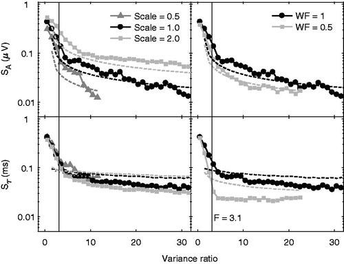
Figure 6 shows the standard error of the wave-V amplitudes and latencies as a function of the F_MP background noise variance. Due to the distribution of the background noise variances, the standard deviation was calculated here within equally spaced logarithmic intervals of background noise variance³. The upper panels show that the standard deviation of the amplitude error, S_A, does not depend on the ABR amplitude (scaling) and width (sharpness of the peak) when shown as a function of the residual noise level. In contrast, the lower right panel shows that S_τ as a function of residual noise varies with the ABR width, even though the effect seems to disappear at high noise levels. Similarly, lower left panel of Figure 6 shows that the standard deviation of the latency error, S_τ, depends on the ABR amplitude when plotted as a function of the residual noise level. The abscissae in Figure 6 are inverted such that high residual noise is represented on the left and low residual noise is represented on the right for an easier comparison with Figure 5. The vertical line indicates a residual noise level of 30 nV. This can be considered a practical noise target for determining no-response situations (i.e. ABR absent) when recording ABRs.

Figure 6. Upper panels show standard error of the wave-V amplitude estimate (S_A), as a function of residual noise variance when scaling the signal and reducing wave-V width, respectively. Lower panels show standard error of the wave-V latency estimate (S_τ), as a function of residual noise variance when scaling the signal and reducing wave-V width, respectively. The vertical lines show a residual noise floor of 30 nV, a practical noise target for no-response situations.

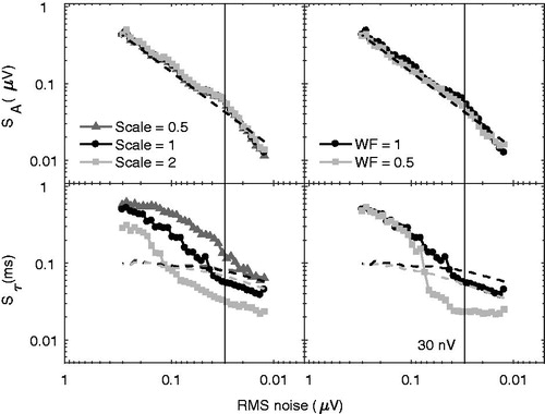
In summary, S_A was found to be sensitive to differences in ABR amplitude and width for a fixed variance ratio but not for a fixed residual noise level. In contrast, for a fixed variance ratio, latency estimates were found to be insensitive to scaling but sensitive to differences in ABR width. Furthermore, latency estimates were sensitive to both scaling and width for a fixed residual noise level.

Discussion

Through synchronous and weighted averaging in AEP recordings the noise floor is reduced relative to the signal of interest. Errors or uncertainty in the post-average waveforms are determined by the residual noise floor and signal-to-noise-ratio of the waveforms. The approach used in this study was to simulate typical ABR recordings in varied noise conditions, by building a large representative EEG database and adding a known template ABR waveform. This provided complete a priori knowledge of the waveform and the wave-V peak amplitude and latency and allowed the exploration of the properties and reliability of the signal quality and residual noise floor estimators.

Comparison of F-ratio methods

The four different noise floor estimates were also used to calculate the weights for the averaging procedure (Elberling and Wahlgreen 1985), which resulted in different post-average waveforms for each of the four methods. Thus, both the numerator and denominator in the variance ratio vary due to the different noise estimation methods employed.

In the numerical experiment, the results for epochs averaged in blocks of 32 were presented. Additional simulations using block sizes of 16, 64, 128 and 256 epochs, revealed that the main trends were independent of block size. At low F-ratios, the amplitude estimate (Figure 3) were more often found to be larger than the true amplitude, i.e. was biased towards positive errors. This resulted from the automatic calculation of the wave-V amplitude as the difference between the largest peak and the smallest trough within ±1 ms of the known true peak and trough location. At very low F-ratios (i.e. high noise floors), the post-averaged waveform is mainly noise whose properties dominate the error and lead to a bias in the amplitude errors.

Above an F-ratio of 3.1 the distribution of errors becomes more symmetrical and is unbiased. At an F_MP value of 3.1, the bias was 0.07 μV, corresponding to 1.43% of the true amplitude (recall A_V,true= 0.488 μV). Therefore, an amplitude bias at realistic F-ratios (as used for clinical applications; 3.1 is the value where an automatic ABR detection algorithm would indicate a signal as present) should not be problematic. The distribution of latency errors (lower panels of Figure 3) was symmetric with respect to the mean, i.e. no systematic bias was observed. This confirms that for an F-ratio greater than 3.1, the error distribution on amplitude and latency becomes rapidly more narrow.

From the comparison of the standard errors across F-ratio estimators (Figure 3), only a little or no difference was found between the performances of the four methods. The accuracy of the simplest algorithms was comparable to that of the most complex algorithm. Therefore, implementation and usage of the NSF_MP algorithm whose computational load surpasses the other algorithms by far does not seem to provide extra benefit when considering accuracy alone. The results from the present study suggest the use of the classic F_MP or the F_SP since they offer a good compromise between accuracy and computational complexity. It is possible that the NSF_MP algorithm is beneficial in terms of detection statistics as suggested by Silva (2009). However, though this seems to be the case in comparison to the F_SP algorithm, it is questionable if the NSF_MP would be advantageous in comparison to the F_MP algorithm.

Averaging stop criteria

It was shown that the amplitude standard error was independent of scaling of the amplitude and compression of the width of the ABR template when shown as a function of residual noise level (upper panels of Figure 6). This suggests that fixed residual noise is an appropriate stopping criterion when the primary interest is on wave-V amplitude. An interesting finding was that the error on the wave-V latency was not a simple function of the residual noise. The latency standard error results tended to support a fixed F-ratio stopping criterion (lower panels of Figure 6), which is insensitive to ABR amplitude (scaling) but sensitive to width. This suggests the use of the F-ratio as a stop criterion for latency measurements to obtain a comparable accuracy although neither the variance ratio or residual noise level seems to be an optimal stop criterion for latency measurements. Thus, depending on the target feature of the ABR useful for the experimental hypothesis or clinical decision, a different stopping criterion is advocated from the results of this study.

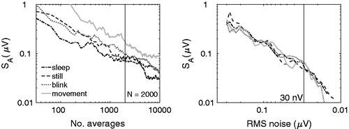
Figure 7 shows a comparison of amplitude standard errors for a fixed number of epochs in the average (left panel) and a fixed residual noise floor as stopping criterion (right panel) when using the F_MP. The figure clearly highlights the well-known but largely ignored disadvantage of only using a fixed number of averages. In cases of increased noise, i.e. test subject movement, the quality of the resultant ABR waveforms varies. If a fixed residual noise were used then this difference in waveform quality would be reduced. To generate Figure 7, no artefact rejection was used in order to highlight the effect of using a fixed number of epochs in the average. In all other stimulations in this study, a strict artefact rejection of 20 μV was used. The variation in amplitude standard error across test subject conditions is significant but relatively modest due to Bayesian averaging. Without Bayesian averaging the impact of high noise epochs within the fixed number of epochs within the average would be greater than the difference shown in Figure 7.

Figure 7. Standard error of the wave-V amplitude estimates (S_A), for the four different background noise cases used in the EEG database and shown as a function of number of averages (left panel) and residual noise floor (right panel). The vertical lines show a residual noise floor of 2000 averages or 30 nV, commonly used targets for ABR recording.

Theoretical predictions of amplitude and latency standard error

In Hoth (1986), theoretical general formulas for the accuracy (standard error) of amplitude and latency estimates from ABR recordings were derived. These were tested against the numerical approach used in this paper, to determine if these closed-form predictions could be usable for routine ABR recordings. They predicted that the standard error of the amplitude can be given by: (7) where σ_n is the residual post-averaged noise standard deviation (RMS). See appendix in Supplementary material for the derivation of the squared error on wave-V peak latency from Hoth (1986). Through a series of simplifications, also described in the appendix in Supplementary material, the predicted latency standard error is given by: (8) where σ_n is the residual post-averaged noise standard deviation, σ_n is the standard deviation of the noise curvature (second derivative w.r.t. time) and is the local curvature of the post-averaged signal at the estimated wave-V latency, t_e.

To use Equations 7(7) and 8(8) an estimate is needed for the post-averaged residual noise standard deviation (σ_n). The sample variance of a 5 ms pre-stimulus interval was used here, as suggested by Hoth (1986). Next, the second derivative of the post-averaged waveform needs to be calculated numerically via a finite difference approximation (see Riley, Hobson, and Bence 1998). was estimated from the 5 ms pre-stimulus interval of and the curvature of the estimated wave-V peak is given by Hoth’s (1986) estimates of the standard errors were calculated and are shown as the dashed curves in Figures 5 and 6 shaded according to the true signal scale or width factors. S_{A, Hoth} as a function of fixed residual noise floor appears to show agreement with the direct numerical results of the present study. S_{A, Hoth} as a function of fixed F-ratio seems to under-predict the direct numerical results. This is a result of the 5 ms pre-stimulus interval used being insufficiently long to accurately estimate the residual noise. EEG is dominated by low frequencies, with an approximate 1/f spectrum (Pritchard 1992). A 5 ms window will only be able to accurately estimate energy down to around 0.2 kHz (McDowell et al. (2007) and will lead to an under-prediction. Simply estimating post-averaged residual noise floor using the multiple point method (see appendix in Supplementary material) will eliminate this problem, making S_{A, Hoth} a useful predictor. Alternative approaches would be to either increase window length from 5 to 30 ms (resulting in very slow ABR acquisition due to much lower stimulus repetition rate) or increase the high-pass filter cut-off to 0.3 kHz (as used in Hoth 1986). However, given that there is useful energy in the ABR down to approximately 30 Hz this choice of filter cut-off would lead to a reduced wave-V amplitude, and is therefore not recommended. Thus, the Hoth (1986) amplitude error predictor is useful if one of the approaches suggested above to improve the accuracy of the sample variance is used.

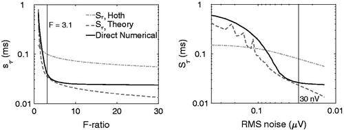
Unlike for the amplitude, S_{τ ,Hoth} is not qualitatively similar to the numerical results from this study. To investigate this, it was necessary to consider the underlying assumptions used in Hoth (1986) to derive an estimate for latency standard error (see Appendix in Supplementary material). A further simulation was carried out explicitly calculating the squared error term in (A14), then giving the latency standard error as the square-root of the expectation (ensemble mean) (Bendat and Piersol 1971) of the squared error: (9)

This calculation is only possible in simulations as it requires knowledge of the true ABR wave-V curvature as well as the true latency, t_L, thus S_{τ ,Theory} is not a useful estimator in practice. A spectrally white Gaussian random sample was generated in MATLAB and filtered to have the same power spectral density as the mean across subjects and runs in the EEG database. An ABR template was added and wave-V peak latency errors were directly determined as well as S_{τ , Theory}. It can be seen in Figure 8 that S_{τ ,Theory} yields a much closer estimate of the latency standard error than S_{τ ,Hoth}. Considering Equation 9(9) , if the additive post-averaged EEG noise is a zero-mean Gaussian random variable with variance σ_n², then θ will also be a Gaussian random variable, i.e. it will also be zero mean. However, it will have a variance dependent on the time separation of the estimated and true latencies as well as the correlation coefficient of the residual noise. It can be shown that ϕ will also be normally distributed but with a non-zero mean and a variance given by Further, it cannot be assumed that θ and ϕ are uncorrelated, nor can the ratio be assumed to be a Gaussian distribution (Hinkley 1969; Hayya, Armstrong, and Gressis 1975). From the simulation results presented here, it does not appear to be reasonable to make the simplifications (see appendix in Supplementary material) where θ is replaced by (i.e. not taking into account the correlation between the two noise terms) nor ϕ by to convert Equation A14 into Equation 8(8) This fails to take into account the PSD of real EEG and its finite and significant correlation length, nor the expected non-Gaussian distribution of the ratio. On the basis of these results, it is not recommended to use the closed-form predictions, S_{τ ,Hoth}, of the latency standard error. Changing the high-pass filter cut-off frequency does not lead to the improved performance with the Hoth (1986) latency error predictor (simulation carried out but not shown for brevity), as seen with the amplitude error predictor. As discussed above, there are several errors in the assumptions used to derive the latency error predictor. Changing the filter settings cannot address this.

Figure 8. Standard error of the wave-V latency (S_τ), calculated numerically, directly according to the theory from Hoth (1986) and as a simplified closed form solution and shown as a function of F-ratio (left panel) and residual noise floor (right panel).

Conclusion

The performance of four different SNR estimation algorithms was investigated and only small differences in performance were found for different degrees of non-encephalic and encephalic noise. Thus, the classic F_SP or the F_MP algorithms seem to offer a good compromise between accuracy and computational load. The main finding of the paper was that the optimal stop criterion (fixed SNR versus fixed noise floor) for comparing results between test subjects of stimulus conditions depends on whether ABR wave-V amplitude or latency is the outcome measure considered. This finding has significance for both clinical and future research studies using the ABR. The reliability of the wave-V amplitude estimate was found to be unaffected by changes to the amplitude and sharpness of the ABR peak for a fixed noise variance but was observed to be sensitive to such changes of the ABR peak for a fixed SNR. In contrast, the reliability of the latency estimate was found to be insensitive to scaling but sensitive to changes to the sharpness of the ABR peak for fixed SNR and to be affected by both differences in scaling and peak sharpness for a fixed residual noise level. This suggests using a fixed noise level as a stop criterion for amplitude measurements and a fixed SNR as a stop criterion for latency measurements. Finally, an investigation was made into signal-based methods for estimating the random errors on amplitude and latency using the post-averaged ABR waveform (Hoth 1986). It was found that the estimated amplitude standard error was in good agreement with the numerical results of the present study and could be further improved using the multiple-point post-averaged residual noise estimates. However, the theoretical validity of the signal-based latency random error estimate is questionable and its use is not recommended without further investigation.

Declaration of interest

The authors report no conflicts of interest.

This work was supported by the Carlsbergfondet and Oticon Foundation.

Supplementary material available online

Acknowledgements

We thank Prof. Ross Roeser and three anonymous reviewers for helpful comments.

Notes

Notes

1. In this paper, the signal-to-noise-ratio (SNR) is simply defined as the ratio of the root-mean-square (RMS) value of the true signal, σ_s(t), divided by the RMS value of the post-averaged residual noise, σ_n(t).

2. Strictly, the latency errors should be modelled by a binomial distribution due to the small number of discrete values it can take due to the sampling interval. However, for simplicity a continuous normal approximation will be made so that the sample variance can be used.

3. It was seen, that the use of linearly spaced noise level intervals would lead to a very uneven distribution of the estimated amplitudes or latencies. By using a logarithmic scale the different estimated variance ratios would be spread more evenly over a larger number of intervals.

References

- Bendat, J. S., and A. G. Piersol. 1971. Random Data: Analysis and Measurement Procedures. Hoboken (NJ): Wiley-Blackwell.
- Burkard, R., and K. E. Hecox. 1987. “The Effect of Broadband Noise on the Human Brainstem Auditory Evoked Response: III. Anatomical Locus.” The Journal of the Acoustical Society of America 81: 1050–1063.
- Carling, K. 2000. “Resistant Outlier Rules and the Non-Gaussian Case.” Computational Statistics and Data Analysis 33: 249–258.
- Davila, C. E., and M. S. Mobin. 1992. “Weighted Averaging of Evoked Potentials.” IEEE Transactions on Bio-Medical Engineering 39: 338–345.
- Don, M., and C. Elberling. 1994. “Evaluating Residual Background-Noise in Human Auditory Brain-Stem Responses.” The Journal of the Acoustical Society of America 96: 2746–2757.
- Don, M., A. R. Allen, and A. Starr. 1977. “Effect of Click Rate on the Latency of Auditory brain stem responses in humans.” The Annals of Otology, Rhinology, and Laryngology 86: 186–195.
- Elberling, C., and M. Don. 1984. “Quality Estimation of Averaged Auditory Brainstem Responses.” Scandinavian Audiology 13: 187–197.
- Elberling, C., and M. Don. 2008. “Auditory Brainstem Responses to a Chirp Stimulus Designed from Derived-Band Latencies in Normal-Hearing Subjects.” The Journal of the Acoustical Society of America 124: 3022–3037.
- Elberling, C., and O. Wahlgreen. 1985. “Estimation of Auditory Brain-Stem Response, ABR, by Means of Bayesian Inference.” Scandinavian Audiology 14: 89–96.
- Elberling, C., J. Callø, and M. Don. 2010. “Evaluating Auditory Brainstem Responses to Different Chirp Stimuli at Three Levels of Stimulation.” The Journal of the Acoustical Society of America 128: 215–223.
- Elberling, C., M. Don, M. Cebulla, and E. Stürzebecher. 2007. “Auditory Steady-State Responses to Chirp Stimuli Based on Cochlear Traveling Wave Delay.” The Journal of the Acoustical Society of America 122: 2772–2785.
- Hayya, J., D. Armstrong, and N. Gressis. 1975. “A Note on the Ratio of Two Normally Distributed Variables.” Management Science 21: 1338–1341.
- Hinkley, D. V. 1969. “On Ratio of 2 Correlated Normal Random Variables.” Biometrika 56: 635.
- Hoth, S. 1986. “Reliability of Latency and Amplitude Values of Auditory-Evoked Potentials.” Audiology: Official Organ of the International Society of Audiology 25: 248–257.
- ISO 389-6. 2007. Acoustics: Reference Zero for the Calibration of Audiometric Equipment – Part 6: Reference Equivalent Threshold of Hearing for Test Signals of Short Duration. Geneva: International Organization for Standardization.
- Lutkenhöner, B., M. Hoke, and C. Pantev. 1985. “Possibilities and Limitations of Weighted Averaging.” Biological Cybernetics 52: 409–416.
- McDowell, E. J., X. Q. Cui, Z. Yaqoob, and C. H. Yang. 2007. “A Generalized Noise Variance Analysis Model and its Application to the Characterization of 1/f Noise.” Optics Express 15: 3833–3848.
- Mühler, R., and H. von Specht. 1999. “Sorted Averaging: Principle and Application to Auditory Brainstem Responses.” Scandinavian Audiology 28: 145–149.
- Picton, T. W., S. A. Hillyard, H. I. Krausz, and R. Galambos. 1974. “Human Auditory EvokedPotentials: I. Evaluation of the Components.” Electroencephalography and Clinical Neurophysiology 36: 179–190.
- Pritchard, W. S. 1992. “The Brain in Fractal Time: 1/f-Like Power Spectrum Scaling of the Human Electroencephalogram.” The International Journal of Neuroscience 66: 119–129.
- Riedel, H., G. Granzow, and B. Kollmeier. 2001. “Single-Sweep-Based Methods to Improve the Quality of Auditory Brain Stem Responses Part II: Averaging Methods.” Zeitschrift Für Audiologie/Audiological Acoustics 40: 62–85.
- Riley, K. F., M. P. Hobson, and S. J. Bence. 1998. Mathematical Methods for Physics and Engineering. Cambridge, UK: Cambridge University Press.
- Silva, I. 2009. “Estimation of Postaverage SNR from Evoked Responses under Nonstationary Noise.” IEEE Transactions on Bio-Medical Engineering 56: 2123–2130.
- Stürzebecher, E., M. Cebulla, and K. D. Wernecke. 2001. “Objective Detection of Transiently Evoked Otoacoustic Emissions.” Scandinavian Audiology 30: 78–88.
- Wong, P. K. H., and R. G. Bickford. 1980. “Brain Stem Auditory Evoked Potentials: The Use of Noise Estimate.” Electroencephalography and Clinical Neurophysiology 50: 25–34.