Subjective evaluation of single microphone noise reduction with different time constants

Abstract

Objective: Previous studies on single microphone noise reduction (NR) in hearing aids (HAs) have shown that some NR algorithms provide beneficial effects in terms of listener preference. To improve HA user satisfaction, we are interested in characteristics that determine preferences for NR, and in the inter-individual variability. The aim of this study was to test if dynamic properties of NR influence listener preference.

Design: The gain reduction at speech offsets of a NR algorithm was slowed down by applying temporal exponential smoothing. At speech onsets the gain recovery was left unchanged. Test signals consisted of speech in continuous and modulated speech-shaped background noise, processed with three time constants: 0, 100, and 200 ms.

Study sample: 16 Normal hearing (NH) and 16 hearing impaired (HI) subjects participated in a paired-comparison listening test.

Results: NH subjects as a group had a significant preference for NR with time constants of 100, or 200 ms (slower acting NR). HI listeners as a group preferred NR over no NR, but had no clear preference for fast or slow NR. Patterns of preference differed between individual listeners.

Conclusions: NR dynamics had an impact on individual listener preference and should be considered when optimising HAs.

Keywords:

• Hearing aids
• hearing aid satisfaction
• listener preference
• noise

Introduction

The experienced difficulty while listening in noisy situations remains one of the main complaints amongst hearing aid users (Gygi and Ann Hall 2016; Vuorialho et al. 2006). To reduce unwanted background noise, current hearing aid (HA) implementations have noise-reduction algorithms such as single-microphone noise reduction (NR). If an input signal is disturbed with noise, the noise-reduction algorithm is designed to improve the overall signal-to-noise ratio (SNR) by reducing the hearing aid’s gain in noise-dominated frequency bands. Such NR algorithms are complex and details of the design parameters are commonly not provided by HA manufacturers. Even so, knowledge of the perceptual effects of NR algorithms is desired for the clinician to facilitate the choice of an optimal hearing aid algorithm for the individual hearingaid user and to select the optimal setting of the chosen NR algorithm. Previously, several studies were conducted in order to evaluate the performance of different NR algorithms. It has been well documented that NR algorithms do not necessarily improve speech intelligibility (Hu and Loizou 2007; Loizou and Kim 2011). However, there is ample evidence that NR can improve subjective experiences such as listening comfort, listening effort or noise annoyance (Brons, Dreschler, and Houben 2014; Desjardins and Doherty 2014; Huber et al. 2018). These improvements can be considered key factors underlying a user’s satisfaction with his/her hearing aid. Results of studies on subjective listening experience are often difficult to interpret, as many parameters influence a person’s final judgment. A common approach to ease interpretation is to isolate and manipulate a single parameter to be able to infer a causal relation with subjective listening experience. Examples of such NR parameters are the type of noise estimator (Brons, Houben, and Dreschler 2012), the interaction with other HA signal processing such as compression (Kortlang et al. 2018), or gain reduction strength. Regarding the latter, previous research on perceptual effects has shown a large variability of preferences for the maximum strength of gain reduction between listeners (Houben, Dijkstra, and Dreschler 2013; Brons, Dreschler, and Houben 2014; Neher and Wagener 2016). Due to noise estimation errors and processing artefacts, stronger noise reduction is accompanied with distortions that reduce speech quality (Bentler et al. 2008). The preferred amount of gain reduction is therefore a trade-off between the amount of noise that is reduced and the amount of distortions one is willing to tolerate. Individuals can weigh these factors differently, which roughly results in two profiles of listeners; those who want a lot of gain reduction in spite of signal distortions and those who want to preserve speech quality in spite of the higher noise levels present (Brons, Houben, and Dreschler 2013).

Another, less well investigated parameter are the time constants by which the NR algorithm changes the gain (Bentler and Chiou 2006; Chung 2004). For amplitude compression in HAs, time constant settings have been shown to affect speech intelligibility as well as listening comfort (Hansen 2002; Moore et al. 2004; Neuman et al. 1995). For NR it is not known if time constants influence the preferences of the listener. Only little research has been done with respect to time constants in NR and their perceptual effects in the user of the HA. Most research focussed on the use of ideal NR algorithms or on comparisons of different NR schemes with each other, rather than directly manipulating the time constants in one non-ideal algorithm (Anzalone et al. 2006; Galster and Ricketts 2004). Also, the focus of these studies was on speech recognition rather than on listener preference. In this study, we intend to investigate the subjective effects of NR time constants in order to learn about the relations between processing speed and listener preference.

Both normal hearing (NH) and hearing impaired (HI) listeners are included in this study. We are interested in the effect of time constants in NR for the two groups as well as in the inter-individual variability. Furthermore, we want to explore whether the trade-off between noise annoyance and speech naturalness that was found in other experiments is also present when testing preferences for NR time constants. Therefore, we will use the paired comparison method to address the following research questions.

• Q1: Do listeners prefer specific time constants?

• Q2: Do individual preferences differ between listeners?

Methods

This research was approved by the medical ethics committee (METC) of the AMC with approval number 2016_061#B2016226. All participants provided a written informed consent.

Subjects

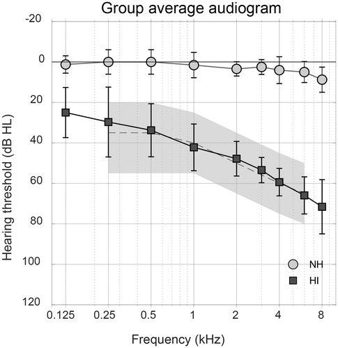
16 normal hearing (NH) and 16 hearing impaired (HI) subjects were included in the experiment. The NH participants (mean age 32.1 ± 10.5 years) were recruited via in-house advertisements and had hearing thresholds of 15 dB HL or better at all octave frequencies between 125 and 8000 Hz. HI participants (mean age 65.4 ± 6.1 years) were recruited via the patient database of the Audiological Centre at Amsterdam UMC, location AMC. They were experienced HA users with a sloping hearing loss that could be classified as N3 according to the classification of Bisgaard, Vlaming, and Dahlquist (2010).All participants were native Dutch speakers. Subjects participated with the ear that had either the better hearing thresholds (in the NH participants) or that was closest to the N3 classification (for the HI participants). The average audiograms of the included ears for NH and HI subjects are shown in Figure 1.

Figure 1. Group averaged audiograms of the tested ears for NH and HI subjects with inter-individual standard deviations. The grey area shows the range of standard audiograms, from N2 to N4, where the dashed line represents the N3 standard audiogram (Bisgaard, Vlaming, and Dahlquist 2010).

Stimuli and signal processing

Input stimuli

Speech material consisted of sentences of Dutch female speech in continuous or modulated background noise. The continuous background noise was a speech shaped noise (SSN), which is a stationary noise with the same long-term power spectrum as the speech materials (Versfeld et al. 2000). The modulated noise was this same SSN that was 50% modulated with a sine wave at a frequency of 1 and 4 Hz. HI listeners were tested with a constant noise and a modulated noise at a frequency of 4 Hz only, to reduce testing time and burden. A modulation depth of 50% was used to have background noise present at all times. The modulation frequency of 4 Hz was chosen because the dominant peak of the amplitude modulation spectrum of natural speech of a single speaker is typically found around 4 Hz (Houtgast 1989). All noise types were summed with the clean speech signal at a long-term SNR of +4 dB. We chose this SNR because we wanted to determine subjective preferences for an SNR that is representative for many real-life situations while speech is still intelligible (Wu et al. 2018). For the modulated background noises this means that the SNR in the peaks and valleys of the noise fluctuated from +0.5 to +10 dB.

Noise reduction algorithm

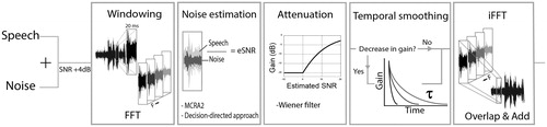
All processing was done in Matlab (v R2016b). All sound signals had a sampling frequency of 44.1 kHz. Time–frequency units were calculated using Fast Fourier transformation (FFT), with 20-ms Hamming-window segments that had a 50% overlap resulting in 882 frequency bins. Subsequent processing occurred in each time–frequency unit. The processing and the NR algorithm is schematically shown in Figure 2 An updated minima-controlled recursive algorithm (MCRA-2) by Rangachari and Loizou was used as a noise estimator for the NR algorithm (Rangachari and Loizou 2006). All initial parameters introduced in this algorithm are kept equal to their default values with an exception of the constants α_d and α_p, that were set to 0.7 and 0.97 respectively, as suggested by Li and Lei (2007). The decision directed approach was used for estimating the SNR, with a weighting factor α = 0.97 (Ephraim and Malah 1984). The linear gain in each time–frequency bin, $G_{t,k}^{\mathrm{ORG}},$ was determined based on the estimated SNR$,\mathrm{ }{\text{ eSNR}}_{t,k}$ with a logarithmic filter similar to a Wiener filter (Brons, Dreschler, and Houben 2014): (1) $$G_{t,k}^{\mathrm{ORG}}={\left(\frac{\max (1,{\mathrm{ }\mathrm{eSNR}}_{t,k})}{1+\max (1,{\mathrm{ }\mathrm{eSNR}}_{t,k})}\right)}^{\beta }$$(1) (2) $$\beta =\frac{-A_{\max }\left(\mathrm{dB}\right)}{20\mathrm{ }\log 10\left(0.5\right)}$$(2)

Figure 2. Block diagram of the NR algorithm used in this study. Each panel corresponds to essential steps in the signal processing. Temporal smoothing is introduced in the fourth panel. Here, the algorithm checks whether there is a decrease in gain with respect to the previous time-frame. If there is (yes), the new gain will be calculated with time constant τ. If there is no decrease in gain (no), the gain will not be altered in this panel.

In Equation (2)(2) $$\beta =\frac{-A_{\max }\left(\mathrm{dB}\right)}{20\mathrm{ }\log 10\left(0.5\right)}$$(2) , the maximum attenuation A_max was set at 20 dB, in order to obtain the largest effect of the temporal settings within the range of realistic applied attenuation in HAs (Chung 2004). At estimated SNRs < 0 dB (${\text{ eSNR}}_{t,k}$<1), the gain reduction was fixed at A_max. Note that in Equation (1)(1) $$G_{t,k}^{\mathrm{ORG}}={\left(\frac{\max (1,{\mathrm{ }\mathrm{eSNR}}_{t,k})}{1+\max (1,{\mathrm{ }\mathrm{eSNR}}_{t,k})}\right)}^{\beta }$$(1) , the maximum value for $G_{t,k}^{\mathrm{ORG}}$ equals 1, which means that the signals are only attenuated or preserved, but not amplified.

As noted, the processing speed in NR is determined by the NR time constants. These time constants are often embedded deep in the algorithm. Examples include smoothing constants involved in the first steps of a NR algorithm, such as the noise estimator (Rangachari and Loizou 2006), or the SNR estimator (e.g. The decision directed approach (Ephraim and Malah 1984)). Altering these constants in a research set-up complicates interpretation of the results because the time constants of the different algorithm components can interact in a complex manner. In order to isolate the effects of time constants within NR, we applied an additional time constant as a final step in the NR algorithm. Thus we do not manipulate the time constants embedded in the algorithms, instead we slow down the gain change with a single time-constant to determine which speed of changes is preferred by listeners. This additional time constant was introduced by means of exponential smoothing of the original gain reduction $G_t^{\mathrm{ORG}}$ determined by the NR algorithm, as shown in Equation (1)(1) $$G_{t,k}^{\mathrm{ORG}}={\left(\frac{\max (1,{\mathrm{ }\mathrm{eSNR}}_{t,k})}{1+\max (1,{\mathrm{ }\mathrm{eSNR}}_{t,k})}\right)}^{\beta }$$(1) . Note that we have removed subscript k for simplicity, however we are still working in separate frequency bins. This gain reduction was slowed down with a certain time constant. In each time–frequency unit, smoothed gain $G_t^{\mathrm{TC}}$ was calculated according to the following formula: (3) $$G_t^{\mathrm{TC}}=\left\{\begin{array}{l}{G}_{t-1}^{\mathrm{TC}}+\left(1-e^{-\frac{1}{\tau }}\right)\times \left(G_t^{\mathrm{ORG}}-{\mathrm{G}}_{t-1}^{\mathrm{TC}}\right), G_t^{\mathrm{ORG}} < {\mathrm{G}}_{t-1}^{\mathrm{TC}}\\ G_t^{\mathrm{ORG}}, G_t^{\mathrm{ORG}}\ge {\mathrm{G}}_{t-1}^{\mathrm{TC}}\end{array}\right.$$(3)

In Equation (3)(3) $$G_t^{\mathrm{TC}}=\left\{\begin{array}{l}{G}_{t-1}^{\mathrm{TC}}+\left(1-e^{-\frac{1}{\tau }}\right)\times \left(G_t^{\mathrm{ORG}}-{\mathrm{G}}_{t-1}^{\mathrm{TC}}\right), G_t^{\mathrm{ORG}} < {\mathrm{G}}_{t-1}^{\mathrm{TC}}\\ G_t^{\mathrm{ORG}}, G_t^{\mathrm{ORG}}\ge {\mathrm{G}}_{t-1}^{\mathrm{TC}}\end{array}\right.$$(3) , ${\mathrm{G}}_{t-1}^{\mathit{TC}}$ is the applied gain in the previous time-frame, $G_t^{\mathrm{ORG}}$ is the gain determined by the NR algorithm in the current time-frame and the time constant τ is defined as the time it takes to reach 1/e of $G_t^{\mathrm{ORG}}.$ Equation (3)(3) $$G_t^{\mathrm{TC}}=\left\{\begin{array}{l}{G}_{t-1}^{\mathrm{TC}}+\left(1-e^{-\frac{1}{\tau }}\right)\times \left(G_t^{\mathrm{ORG}}-{\mathrm{G}}_{t-1}^{\mathrm{TC}}\right), G_t^{\mathrm{ORG}} < {\mathrm{G}}_{t-1}^{\mathrm{TC}}\\ G_t^{\mathrm{ORG}}, G_t^{\mathrm{ORG}}\ge {\mathrm{G}}_{t-1}^{\mathrm{TC}}\end{array}\right.$$(3) shows that the gain is only manipulated when it decreases. The resulting reaction of the algorithm to a decrease in SNR is slower for higher values of the time constant τ. A detected increase in SNR is processed without additional smoothing, to ensure fast recovery of gain when speech is detected. Stimuli were processed with three time constants, τ = 0 ms, 100 and 200 ms.

After the final attenuation in each time–frequency unit was determined, the signal was re-synthesized with an inverse FFT and overlap-and-add method (Loizou 2013). The unprocessed input signal was used as reference condition in the listening experiments. Per noise type (continuous and modulated), four conditions were compared consisting of the three time constants and the unprocessed input signal. Processing conditions are labelled TC0, TC100, TC200, and Unpr for τ = 0 ms, 100 ms, 200 ms, and unprocessed signals respectively.

A NR algorithm reduces signal strength. We compensated for this overall attenuation to maintain audibility of speech. All processed stimuli were amplified as such that the power of all processed speech signals was matched to the power of the unprocessed speech signal. This amplification was calculated by using only the speech part of the processed signal that was available from our algorithm.

Figure 3 shows a time–frequency representation of the applied gain of each condition relative to the unprocessed stimulus before overall level correction. This figure illustrates that the degree of temporal smoothing of the gain is larger for the larger time constants. Table 1 shows the output SNRs of all test conditions. All processing conditions showed improved SNRs that were the result of reduced noise levels.

Figure 3. Time–frequency representation of the applied gain due to the NR algorithm, without level corrections. The grey scale in the spectrogram-like plot shows the amount of (negative) gain applied as a result of noise reduction with different time constants. Here, gain is defined as the difference in output per time–frequency unit between the processed and unprocessed condition. On top of the panels, the time signal of the noise reduced sentence in noise is shown for each condition (light-grey signal) combined with the unprocessed sentence in noise (dark-grey signal).

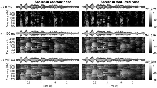
Table 1. Information on processing conditons: average ± standard deviations of the resulting SNR of all processing conditions per noise type.

Conditions	Labels	SNR (dB) Continuous noise	SNR (dB) Modulated noise
τ = 0 ms	TC0	+12.6 ± 0.2	+12.1 ± 0.2
τ = 100 ms	TC100	+10.9 ± 0.1	+10.1 ± 0.1
τ = 200 ms	TC200	+9.9 ± 0.1	+9.2 ± 0.1
Unprocessed	Unpr	+3.9 ± 0.004	+3.9 ± 0.004

SNR calculations were done per list of 13 sentences with a 1 s pause between each sentence. The between-list standard deviations are shown.

Listening tests

After testing hearing thresholds with standard pure tone audiometry, all subjects performed three listening tests. The first two listening tests served as a verification of our test signals to check whether all conditions were intelligible and distinguishable. All listening tests were done in a sound proof booth. Stimuli were presented to the subjects monaurally through Sennheiser HDA200 headphones. Stimuli were presented to NH subjects with an average noise level of 65 dB SPL. The overall presentation level for speech in noise ranged from 69 to 72 dB SPL. HI subjects listened to the stimuli with an additional gain compensation derived from their pure-tone audiogram according to the NAL-RP prescription (Dillon 2001). In this way, amplification is linear and effects of other signal processing features such as amplitude compression can be ruled out.

Speech intelligibility

Speech intelligibility of all conditions was tested. Conditions were played in lists of 13 sentences following one practice list of 13 sentences that contained all processing conditions. The order of processing conditions and lists was randomised and balanced over subjects to avoid training effects on group data. After listening to a sentence the subjects were asked to repeat what they had heard. Speech intelligibility per condition was determined by the percentage correct word repetitions of the last 10 sentences in a list (word scores based on all words in the sentence).

Discrimination

In a discrimination experiment we verified whether test conditions are distinguishable. By means of a three-alternative forced-choice paradigm subjects were asked to detect which stimulus was different from the other two. The same sentence was played three times subsequently in the same noise type, where one was processed with a different time constant than the other two. The subject could listen to the same stimuli once again, after which they had to choose the ‘odd one out’.

Listener preference

Listener preference for three judgment criteria (noise annoyance, speech naturalness and overall preference) was determined by pairwise comparisons. A similar procedure has been described previously by Brons, Houben, and Dreschler (2013). Subjects were asked to listen to two sentences with different processing and answer three subsequent questions: ‘In which of the sentences is the background noise less annoying?’, ‘In which of the sentences does speech sound more natural?’, and ‘Which of the sentences do you like more?’. Answers were given on a 7 point scale. E.g. in the case of the first asked question, subjects could choose whether they thought sentence A or B had ‘a lot less’, ‘less’, or ‘a little less’ annoying background noise. They could also choose to be indifferent between the two comparisons. The four processing conditions were compared within each noise type and all comparisons were repeated three times. In this listening test, level roving (of –1, 0, or +1 dB) was applied to the speech in noise signal to reduce potential effects due to remaining differences in perceived loudness.

Results

Analyses of the results of the two modulating noise conditions in NH listeners revealed no statistical significant differences between the 1 and 4 Hz modulation frequencies in all tests. Therefore, only results of the test conditions with background noises that were tested both in NH and HI participants (constant and 4 Hz modulated noise) are shown.

Speech intelligibility

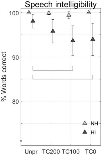
Figure 4 shows the results of the speech intelligibility experiment for all listeners. A repeated measures ANOVA showed no significant effect of noise type and no significant interactions of noise type with processing condition for both groups. Therefore the percentages of correctly repeated words per condition are shown for both noises together. There were no statistically significant differences between conditions for the NH listeners’ intelligibility scores. As indicated by the horizontal bars in Figure 4, HI listeners showed significant differences for processing conditions TC0 and TC100, compared to Unpr, calculated by post-hoc pairwise comparisons after Bonferroni corrections (p = 0.05/6).

Figure 4. Group averages of the speech intelligibility listening test for all listeners and conditions in terms of % correct repeated words. Results per listener group are pooled for both noise types. Error bars show 95% confidence intervals. NH subjects showed no significant differences between processing conditions. Horizontal bars show two significant differences between processing conditions for HI listeners.

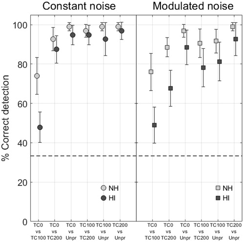
Discrimination

The percentages of correctly detected differences are shown in Figure 5 for both groups of listeners per noise type. Data were transformed using Rationalised Arcsine Units in order to correctly use the percentages in statistical analysis (Studebaker 1985). All comparisons yielded discrimination scores that were significantly higher than chance (33.3%, see dashed horizontal line in Figure 5). This was tested with one-sided t tests assuming that discrimination results are always equal to or greater than chance.

Figure 5. Group average percentage correct detection of all comparisons in the discrimination experiment, for NH and HI listeners. Error bars show 95% confidence intervals, the dashed horizontal line indicates the 33.3% chance level.

Listener preference

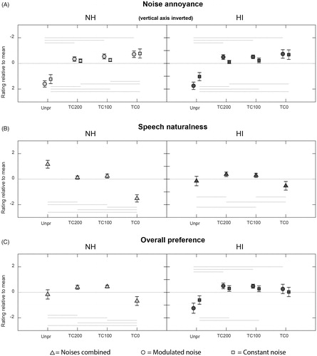
The group average results of the paired comparison test determining listener preference are shown in Figure 6. NH listener results are shown on the left, HI listener results are shown on the right. The figure shows a relative rating for each processing condition per noise type and per judgement criterion (panels A, B and C). For each comparison scores from –3 to +3 were assigned to each condition according to the P.800 ITU-T recommendation (ITU-T 1996). For noise annoyance, the vertical axis has been inverted so that for each condition a rating above zero can be interpreted as having a better performance for the judgement criterion.

Figure 6. Group average results of the paired comparison experiment in NH subjects (left side) and HI subjects (right side) for the two noises and three judgment criteria (A, B, C). When there is a significant interaction between noise type and processing condition, both noise types are shown separately in the figure, otherwise the results are pooled for both noise types. Each condition is rated relative to the mean where the ‘noise annoyance’ scale is inverted. Error bars show 95% confidence intervals. Horizontal bars indicate which conditions differ significantly from each other. Positive values indicate a favorable outcome.

Statistical analysis was performed using the log-linear modelling approach for ordinal paired comparisons (Dittrich, Hatzinger, and Katzenbeisser 2004). This approach is used for dealing with paired-comparison data that has multiple response categories with the inclusion of a “no difference” option. So called ‘worth’ parameters are obtained by fitting our paired-comparison data with this model. These parameters can be used for ranking the preference for the processing conditions and they give information on the strength of preference. A mixed model analysis of variance (ANOVA) on these worth parameters was performed comparing listener groups with processing condition and noise type as fixed effects and subject as random effect. The F and p statistics of these analyses are shown in Table 2 for each judgement criterion.

Table 2. F and p statistics of a mixed model ANOVA of the paired comparison listening test to determine listener preference.

		Noise annoyance		Speech naturalness		Overall preference
Effect	Df	F	p	F	p	F	p
Group (NH or HI)	1	0.04	0.8	23.59	<0.001	9.76	0.004
TC	3	86.25	<0.001	25.82	<0.001	14.34	<0.001
Noise	1	22.39	<0.001	<0.001	>0.9	18.33	0.002
Group × TC	3	0.1	>0.9	18.2	<0.001	8.96	<0.001
Group × Noise	1	2.59	0.1	2.48	0.1	1.42	0.2
TC × Noise	3	8.44	<0.001	1.33	0.3	6.05	<0.001
TC × Subject	90	2.25	<0.001	3.29	<0.001	2.73	<0.001

Statistics of all three judgement criteria are shown for listener group, processing condition (TC), and noise type as well as the interaction effects of group with processing condition or noise type.

Because of the significant interactions of listener group with processing condition for judgement criteria speech naturalness and overall preference, we also performed a repeated measures ANOVA for both listener groups separately. Tables 3 and 4 show the results for NH and HI listeners, respectively.

Table 3. Results of the repeated measures ANOVA of the paired comparison listening test for NH listeners.

		Noise annoyance		Speech naturalness		Overall preference
Effect	df	F	p	F	p	F	p
TC	3	51.16	<0.001	33.42	<0.001	9.57	<0.001
Noise	1	3.64	0.08	0.89	0.4	3.75	0.07
TC × Noise	6	2.7	0.05	1.76	0.2	2.51	0.06

The table shows F and p statistics of all three judgement criteria for processing condition (TC), noise type and the interaction of processing condition with noise type.

Table 4. Results of the repeated measures ANOVA of the paired comparison listening test for HI listeners.

		Noise annoyance		Speech naturalness		Overall preference
Effect	df	F	p	F	p	F	P
TC	3	37.3	<0.001	4.56	0.007	13.47	<0.001
Noise	1	30.45	<0.001	2.07	0.2	20.56	<0.001
TC × Noise	6	6.04	<0.001	1.36	0.3	4.67	0.003

The table shows F and p statistics of all three judgement criteria for processing condition (TC), noise type and the interaction of processing condition with noise type.

For NH listeners there was a significant effect of processing condition in each judgement criterion. The effect of noise type was not significant for either of the judgement criteria and the interaction of processing condition with noise type was only significant for noise annoyance.

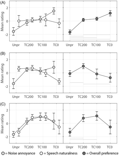
For HI listeners there were significant effects of processing conditions and noise types in all judgement criteria with an exception of the effects of the type of background noise on speech naturalness. Also, the interaction of processing condition with noise type was not significant for the criterion of speech naturalness. Horizontal lines in Figure 6 indicate which conditions differ significantly from each other after post-hoc pairwise comparisons with Bonferroni corrections (p = 0.05/6). Figure 7 shows the paired comparison results of three HI individuals (A, B, C) for all processing conditions in both noise types, illustrating the differences between individuals. The judgement criteria “noise annoyance” and “speech naturalness”, are shown on the left side of the figure. On the right side the judgement criterion “overall preference” is shown. For this criterion we have performed post hoc pairwise comparisons to indicate which condition differs significantly from each other (p = 0.05), shown with horizontal lines. Bonferroni corrections were not applied because of the very small data set. These particular three participants were chosen as they were considered to be representing the broad spectrum of individual preferences.

Figure 7. Paired comparison results of three HI individuals (A, B, C) for all processing conditions for both noise types combined. The vertical axis shows a relative rating for each processing condition which is based on the mean of three runs per comparison. Error bars show 95% confidence intervals. Speech naturalness ratings are shown with white markers, noise annoyance ratings with light-grey markers, both on the left side of the figure. The overall preference ratings are shown separately on the right side of the figure with dark-grey markers. Note that for the noise annoyance rating one should interpret a negative value on the y-axis as more annoying than a positive value on the y-axis. Horizontal bars indicate which conditions differ significantly from each other, for α = 0.05. Positive values indicate a favorable outcome.

Discussion

In the speech intelligibility listening test NH listeners scored close to 100% correct for all test conditions and HI listeners on average scored above 90% correct. With the chosen SNR (+4 dB SNR) the high results for speech intelligibility for both listener groups were intentional and merely a verification of the processing conditions. For HI listeners intelligibility scores for unprocessed signals were significantly better than TC0 and TC100 in spite of the calculated SNR improvements that can be found in Table 1. This effect is in agreement with other studies that explain that intelligibility is not only related to the SNR but also to the amount of distortions present in the signal (Hu and Loizou 2007; Loizou and Kim 2011). Furthermore, the NR algorithm is mainly removing noise that is not masking the speech, thereby improving the calculated overall SNR but not making more speech information available to the listener.

In the discrimination test all comparisons were well above chance level, which implies that all test conditions were distinguishable. For all data points the HI group had poorer scores than the NH group, which is consistent with findings of Brons et al. where HI listeners had higher detection thresholds for NR processing (Brons, Dreschler, and Houben 2014).

Q1: Do listeners prefer specific time constants?

Figure 6C (left) shows that NH listeners prefer the settings TC100 and TC200 over TC0 and unprocessed signals. This implies a beneficial effect from temporal exponential smoothing. We hypothesise that a form of sound distortion called ‘roughness’ can explain the preference for longer time constants. This is a term that refers to amplitude modulations with frequencies between 20 and 200 Hz that are commonly perceived as unpleasant (De Baene et al. 2004). These amplitude modulations are initially present in the TC0 condition, however they are reduced due to the temporal smoothing applied in conditions TC100 and TC200. Spectral analysis of the amplitude modulations of our stimuli has shown that there is a significant reduction of amplitude modulation frequencies between 20 and 30 Hz for both conditions TC100 and TC200 with respect to TC0. This could result in a preference for the slower processing conditions. Also, slower processing reduces the undesirable ‘pumping’ effect (Chung 2004). Another noticeable effect of the processing in TC100 and TC200 is the introduction of reverberation, which is known to be appreciated as more natural (Begault and Trejo 2000). In Figure 6B (left) we see that speech processed by TC100 and TC200 is judged significantly more natural than speech processed by TC0. In combination with the unpleasant roughness of the fast amplitude modulations and the pumping effect in TC0, it is plausible that this condition is the least preferred, together with the unprocessed condition. To our knowledge no similar studies on subjective effects of varying time constants in NR have been published thus far. Therefore these findings cannot directly be compared to findings in literature. However, there are studies that report preferences for slower processing in different set-ups. Bentler et al. (2008) studied preferences for onset times of NR within one HA and reported that in terms of listening comfort a slower onset of a NR algorithm was preferred over a faster onset. It should be noted that these onset times are in the range of seconds and determine the duration of NR activation after noise detection, whereas the time constants in our study are in the range of milliseconds and determine the speed of gain changes within the NR processing. For amplitude compression, the subjective effects of varying time constants have been studied more extensively and these studies report subjective preferences for longer time constants in amplitude compression (Hansen 2002; Neuman et al. 1995).

For HI listeners, Figure 6C (right) shows that the Unpr condition is the least preferred condition even though it is better intelligible, see Figure 4. This suggests that other factors such as listening effort and listening comfort play an important role in determining listener preference. This is in agreement with previous research: Desjardins and Doherty (2014) found a reduction in listening effort with NR when speech-recognition-in-noise scores were not improved, and Brons, Dreschler, and Houben (2014) have found an overall preference for a NR algorithm over unprocessed signals that did not improve speech intelligibility. HI listeners have no significant preference for larger time constants (Figure 6C, right). However, this does not necessarily rule out a positive effect of temporal smoothing in NR. Because roughness perception in HI individuals has been previously shown to be comparable to roughness perception in NH individuals (Tufts and Molis 2007), one would expect a positive effect of smoothing in NR also in both groups. However, the lower scores for % correct detection of differences between processing conditions suggest that the HI listeners in our study are less sensitive than NH to changes in dynamic NR settings. In our stimuli the signal differences might thus be less audible to HI listeners than to NH listeners. Because less difference is heard, perhaps it is more difficult to choose a most preferred setting. In addition, the maximum gain reduction of 20 dB chosen in this study results in a substantial difference between the NR conditions and the unprocessed signals. This high contrast could have masked more subtle differences between NR conditions in the paired-comparison experiment in spite of the applied level corrections.

The paired comparison listening test with a focus on speech naturalness and noise annoyance separately was used to explore the possible trade-off between those factors for determining overall preference. For NH listeners, this trade-off of noise annoyance and speech naturalness is visible: the condition with the most annoying background noise was also rated as the condition with the most natural speech. Likewise, where background noise is least annoying, speech is judged to be the least natural. The resulting overall preference is a balance between the two extremes (of no processing and much processing). Similar results have been shown previously in listener preference experiments (Brons, Houben, and Dreschler 2013). For HI listeners however, this trade-off is less pronounced. As noted above, both listener groups are like-minded concerning noise annoyance. On the other hand, unlike NH listeners, HI listeners judged unprocessed speech in noise to be less natural than TC100 and TC200. These results are in agreement with findings of Huber et al. (2018), who have evaluated the sound quality of nine different NR algorithms. In their study HI listeners judged unprocessed speech in noise as being more distorted than all of the evaluated noise reduced signals. Similar differences between NH and HI listeners for judging speech naturalness have been found by Brons, Dreschler, and Houben (2014) in a paired comparison test where HI listeners rated NR as more natural than unprocessed. A possible explanation is that for HI listeners the rating for speech naturalness is strongly determined by the absence of noise (Marzinzik 2001). This difference in perception of distortions compared to NH listeners might be caused by supra-threshold deficits that accompany hearing loss.

Q2: Do individual preferences differ between listeners?

Several studies have shown large inter-individual differences in subjective listening experiments which implies that group averages may not sufficiently represent the individual preferences (Houben, Dijkstra, and Dreschler 2013; Neuman et al. 1995). The repeated measures ANOVA of the estimated worth parameters of all listeners showed a significant interaction of processing condition with subject (Table 2) for all judgement criteria. Thus, also in this study there is a large variation of preferences between subjects, irrespective of their level of speech understanding. Therefore, group averages for preference such as in Figure 6 should be handled with caution and should not lead to the incorrect conclusion that temporal smoothing in NR does not affect listener preference of individual HA users. The examples of individual results in Figure 7 illustrate this statement. The participant in (A) significantly prefers TC0 over TC200, while the participant in (B) significantly prefers TC200 over TC0. Also the participant in (C) has a stronger preference for the temporally smoothed conditions TC100 and TC200. It is important to consider individual preferences when evaluating HA signal processing features. Since our results apply to a laboratory setting and to limited speech in noise conditions, the results are not directly applicable in clinical practice. If it were possible in hearing aids to change NR time constants, the clinician could present different settings to their client in order to choose the best setting. Unfortunately in clinical practice the options of adapting and fine-tuning NR time constants, and other parameters, are at present rather limited. More research in this area could strengthen the case for individualised NR settings. And that, in turn, might provide a step to improve patient satisfaction with listening to speech in noise.

In Figure 7 we can examine the personal trade-off that is made between speech naturalness and noise annoyance for determining overall preference. The trade-off is shown in the left panels of the figure, with the overall preference in the right panels. For the participant in (A) the overall preference rating is stronger influenced by noise annoyance, while the overall preference rating of the participant in (B) is stronger influenced by speech naturalness. These different preference profiles have been reported previously in literature and can as yet not be related to any objective or subjective measure (Neher and Wagener 2016; Houben, Dijkstra, and Dreschler 2013; Brons, Houben, and Dreschler 2013). For participant (C) however, the ratings of all judgement criteria are rather alike. This listener does not make a similar trade-off between noise annoyance and speech naturalness which suggests that some of the individual listeners may not fit into either one of the preference profile as described above. Untangling the underlying motives for these preference profiles could be, albeit challenging, an interesting direction for future studies. If we can better predict and classify personal listener preferences for NR parameters in the future, we can work towards a more efficient, successful, and individualised HA fitting.

Limitations

Since the mean age was considerably higher in the HI group than in the NH group, we need to consider the effect of age on the results. It is well-established that not only hearing impairment but also aging can have negative effects on performance in noise (Pichora‐Fuller, Schneider, and Daneman 1995; Dubno, Dirks, and Morgan 1984). Therefore, the group differences we found cannot exclusively be attributed to a difference in hearing thresholds.

All tests were performed in a laboratory setting in order to study the effect of temporal smoothing in NR in isolation. Conclusions drawn from this experiment should take into account the limits of our research methods. For example, these results give no insight in the interaction effect with other signal processing features such as amplitude compression. Also, the implications made are limited to the type of processing used in this study: the manipulation of reaction times by means of slowing down a fast NR algorithm. It is unknown how other type of NR algorithms respond to this particular method of introducing time constants.

Although exact values of similar time constants in NR algorithms are unknown, they are commonly within the range of applied time constants (10 ms–10 s) as reported in Chung (2004). Our values of τ fall within this range. On a side note, our values for τ are also comparable to realistic implementations of time constants in amplitude compression (Hansen 2002; Moore et al. 2004). However, given the fact that exact time constants in hearing aids are still unknown, the applicability of our results for clinical practice is limited in the sense that we cannot yet advice on how to adjust or select HA NR. However, our results support understanding of how time constants influence preference and as such provide useful knowledge for clinical practice.

Conclusion

This study provides additional information to the scarcely studied field of NR dynamics. Our results indicate that NH listeners have – on average – a significant preference for temporal smoothed NR with time constants of 100 or 200 ms (slower NR processing). HI listeners prefer NR over unprocessed signals, but we found no group effect of time constants on overall listener preference. At group level, both NH and HI listeners rate shorter time constants as positively reducing noise annoyance, but negatively affecting speech naturalness. Since significant inter-individual differences of preference results were found in HI listeners it is reasonable to assume that NR dynamics can have a large effect on listener preference for some individuals. Therefore individual assessment of different time constants in NR might be beneficial for HA fitting.

Disclosure statement

No potential conflict of interest was reported by the authors.

Additional information

Funding

The authors would like to thank the Heinsius–Houbolt foundation for funding this research.

References

- Anzalone, M. C., L. Calandruccio, K. A. Doherty, and L. H. Carney. 2006. “Determination of the Potential Benefit of Time–Frequency Gain Manipulation.” Ear and Hearing 27 (5): 480–492. doi:10.1097/01.aud.0000233891.86809.df.
- Begault, D. R., and L. J. Trejo. 2000. 3-D sound for virtual reality and multimedia. Moffett Field, CA United States: NASA Ames Research Center.
- Bentler, R., and L. K. Chiou. 2006. “Digital Noise Reduction: An Overview.” Trends in Amplification 10 (2): 67–82. doi:10.1177/1084713806289514.
- Bentler, R., Y.-H. Wu, J. Kettel, and R. Hurtig. 2008. “Digital Noise Reduction: Outcomes from Laboratory and Field Studies.” International Journal of Audiology 47 (8): 447–460. doi:10.1080/14992020802033091.
- Bisgaard, N., M. S. Vlaming, and M. Dahlquist. 2010. “Standard Audiograms for the IEC 60118-15 Measurement Procedure.” Trends in Amplification 14 (2): 113–120. doi:10.1177/1084713810379609.
- Brons, I., W. A. Dreschler, and R. Houben. 2014. “Detection Threshold for Sound Distortion Resulting from Noise Reduction in Normal-Hearing and Hearing-Impaired Listeners.” Journal of the Acoustic Society of America 136 (3): 1375. doi:10.1121/1.4892781.
- Brons, I., R. Houben, and W. A. Dreschler. 2012. “Perceptual Effects of Noise Reduction by Time–Frequency Masking of Noisy Speech.” Journal of the Acoustic Society of America 132 (4): 2690–2699. doi:10.1121/1.4747006.
- Brons, I., R. Houben, and W. A. Dreschler. 2013. “Perceptual Effects of Noise Reduction with respect to Personal Preference, Speech Intelligibility, and Listening Effort.” Earing and Hearing 34 (1): 29–41. doi:10.1097/AUD.0b013e31825f299f.
- Brons, I., R. Houben, and W. A. Dreschler. 2014. “Effects of Noise Reduction on Speech Intelligibility, Perceived Listening Effort, and Personal Preference in Hearing-Impaired Listeners.” Trends in Hearing 18: 1–10. doi:10.1177/:2331216514553924.
- Chung, K. 2004. “Challenges and Recent Developments in Hearing Aids. Part I. Speech Understanding in Noise, Microphone Technologies and Noise Reduction Algorithms.” Trends in Amplification 8 (3): 83–124. https://www.ncbi.nlm.nih.gov/pubmed/15678225 doi:10.1177/108471380400800302.
- De Baene, W., A. Vandierendonck, M. Leman, A. Widmann, and M. Tervaniemi. 2004. “Roughness Perception in Sounds: Behavioral and ERP Evidence.” Biological Psychology 67 (3): 319–330. doi:10.1016/j.biopsycho.2004.01.003.
- Desjardins, J. L., and K. A. Doherty. 2014. “The Effect of Hearing Aid Noise Reduction on Listening Effort in Hearing-Impaired Adults.” Earing and Hearing 35 (6): 600–610. doi:10.1097/AUD.0000000000000028.
- Dillon, H. 2001. Hearing Aids. Australia: Boomerang Press.
- Dittrich, R., R. Hatzinger, and W. Katzenbeisser. 2004. “A Log-Linear Approach for Modelling Ordinal Paired Comparison Data on Motives to Start a PhD Programme.” Statistical Modelling: An International Journal 4 (3): 181–193. doi:10.1191/1471082X04st072oa.
- Dubno, J. R., D. D. Dirks, and D. E. Morgan. 1984. “Effects of Age and Mild Hearing Loss on Speech Recognition in Noise.” The Journal of the Acoustical Society of America 76 (1): 87–96. https://www.ncbi.nlm.nih.gov/pubmed/6747116 doi:10.1121/1.391011.
- Ephraim, Y., and D. Malah. 1984. “Speech Enhancement Using a Minimum-Mean Square Error Short-Time Spectral Amplitude Estimator.” IEEE Transactions on Acoustics, Speech, and Signal Processing 32 (6): 1109–1121. doi:10.1109/TASSP.1984.1164453.
- Galster, J., and T. Ricketts. 2004. “The Effect of Digital Noise Reduction Time Constants on Speech Recognition in Noise. Poster Presented at the 2004 International Hearing Aid Research Conference (IHCON), Lake Tahoe, CA.
- Gygi, B., and D. Ann Hall. 2016. “Background Sounds and Hearing-Aid Users: A Scoping Review.” International Journal of Audiology 55 (1): 1–10. doi:10.3109/14992027.2015.1072773.
- Hansen, M. 2002. “Effects of Multi-Channel Compression Time Constants on Subjectively Perceived Sound Quality and Speech Intelligibility.” Earing and Hearing 23 (4): 369–380. https://www.ncbi.nlm.nih.gov/pubmed/12195179 doi:10.1097/00003446-200208000-00012.
- Houben, R., T. M. Dijkstra, and W. A. Dreschler. 2013. “Analysis of Individual Preferences for Tuning of Noise-Reduction Algorithms.” Journal of the Audio Engineering Society 60 :1024–1037.
- Houtgast, T. 1989. “Frequency Selectivity in Amplitude-Modulation Detection.” Journal of Acoustic Society of America 85 (4): 1676–1680. https://www.ncbi.nlm.nih.gov/pubmed/2708683 doi:10.1121/1.397956.
- Hu, Y., and P. C. Loizou. 2007. “A Comparative Intelligibility Study of Single-Microphone Noise Reduction Algorithms.” Journal of Acoustic Society of America 122 (3): 1777. 2766778 doi:10.1121/1.
- Huber, R., T. Bisitz, T. Gerkmann, et al. 2018. “Comparison of Single-Microphone Noise Reduction Schemes: Can Hearing Impaired Listeners Tell the Difference?” International Journal of Audiology 57: 55–61. doi:10.1080/14992027.2017.1279758.
- ITU-T. 1996. “Methods for Subjective Determination of Transmission Quality.” In Recommendation P.800, edited by Union IT, Geneva: International Telecommunication Union.
- Kortlang, S., Z. Chen, T. Gerkmann, et al. 2018. “Evaluation of Combined Dynamic Compression and Single Channel Noise Reduction for Hearing Aid Applications.” International Journal Audiology 57: S43–S54. doi:10.1080/14992027.2017.1300695.
- Li, C.-W., and S.-F. Lei. 2007. “Signal Subspace Approach for Speech Enhancement in Nonstationary Noises.” ISCIT'07: IEEE International Symposium on Communications and Information Technologies, Sydney, Australia: IEEE. 1580–1585.
- Loizou, P. C. 2013. Speech Enhancement: Theory and Practice. Boca Raton: CRC Press.
- Loizou, P. C., and G. Kim. 2011. “Reasons Why Current Speech-Enhancement Algorithms Do Not Improve Speech Intelligibility and Suggested Solutions.” IEEE Transactions on Audio Speech and Language Processing 19 (1): 47–56. doi:10.1109/Tasl.2010.2045180.
- Marzinzik, M. 2001. Noise Reduction Schemes for Digital Hearing Aids and Their Use for the Hearing Impaired. Oldenburg: Universität Oldenburg.
- Moore, B. C. J., T. H. Stainsby, J. I. Alcántara, and V. Kühnel. 2004. “The Effect on Speech Intelligibility of Varying Compression Time Constants in a Digital Hearing Aid.” International Journal of Audiology 43 (7): 399–409. https://www.ncbi.nlm.nih.gov/pubmed/15515639 doi:10.1080/14992020400050051.
- Neher, T., and K. C. Wagener. 2016. “Investigating Differences in Preferred Noise Reduction Strength among Hearing Aid Users.” Trends in Hearing 20: 2331216516655794. doi:10.1177/2331216516655794.
- Neuman, A. C., M. H. Bakke, C. Mackersie, S. Hellman, and H. Levitt. 1995. “Effect of Release Time in Compression Hearing Aids: Paired‐Comparison Judgments of Quality.” The Journal of the Acoustical Society of America 98 (6): 3182–3187. doi:10.1121/1.413807.
- Pichora‐Fuller, M. K., B. A. Schneider, and M. Daneman. 1995. “How Young and Old Adults Listen to and Remember Speech in Noise.” The Journal of the Acoustical Society of America 97 (1): 593–608. doi:10.1121/1.412282.
- Rangachari, S., and P. C. Loizou. 2006. “A Noise-Estimation Algorithm for Highly Non-Stationary Environments.” Speech Communication 48 (2): 220–231. doi:10.1016/j.specom.2005.08.005.
- Studebaker, G. A. 1985. “A “Rationalized” Arcsine Transform.” Journal of Speech, Language, and Hearing 28 (3): 455–462. https://www.ncbi.nlm.nih.gov/pubmed/4046587 doi:10.1044/jshr.2803.455.
- Tufts, J. B., and M. R. Molis. 2007. “Perception of Roughness by Listeners with Sensorineural Hearing Loss.” The Journal of the Acoustical Society of America 121 (4): EL161–EL167. doi:10.1121/1.2710744.
- Versfeld, N. J., L. Daalder, J. M. Festen, and T. Houtgast. 2000. “Method for the Selection of Sentence Materials for Efficient Measurement of the Speech Reception Threshold.” The Journal of the Acoustical Society of America 107 (3): 1671–1684. doi:10.1121/1.428451.
- Vuorialho, A., M. Sorri, I. Nuojua, and A. Muhli. 2006. “Changes in Hearing Aid Use Over the Past 20 Years.” European Archives of Oto-Rhino-Laryngology: Official Journal of the European Federation of Oto-Rhino-Laryngological Societies (EUFOS): Affiliated with the German Society for Oto-Rhino-Laryngology – Head and Neck Surgery 263 (4): 355–360. doi:10.1007/s00405-005-1007-1.
- Wu, Y.-H., E. Stangl, O. Chipara, S. S. Hasan, A. Welhaven, and J. Oleson. 2018. “Characteristics of Real-World Signal to Noise Ratios and Speech Listening Situations of Older Adults with Mild to Moderate Hearing Loss.” Earing and Hearing 39 (2): 293–304. doi:10.1097/AUD.0000000000000486.