Transient otoacoustic emissions and audiogram fine structure in the extended high-frequency region

Abstract

Objective

Previous studies at conventional audiometric frequencies found associations between the ripple depth seen in audiogram fine structure (AFS) and amplitudes of both transient evoked otoacoustic emissions (TEOAEs) and overall hearing threshold levels (HTLs). These associations are explained by the cochlear mechanical theory of multiple coherent reflections of the travelling wave apically by reflections sites on the basilar membrane and basally by the stapes.

Design

The aim was to investigate whether a similar relationship is seen in the extended high-frequency (EHF) range from 8–16 kHz. Measurements from 8–16 kHz were obtained in normal-hearing subjects comprising EHF HTLs, EHF TEOAEs using a double evoked paradigm, and Bekesy audiometry to assess AFS ripple depth and spectral periodicity.

Study Sample

Twenty eight normal-hearing subjects participated.

Results

Results showed no significant correlation between AFS ripple depth and either frequency-averaged EHF HTLs or EHF TEOAE amplitudes. The amplitude of AFS ripple depth was also lower than that seen in the conventional frequency region and spectral periodicity in the ripple more difficult to discern.

Conclusion

The results suggest a weaker interference pattern between forward and reverse cochlear travelling waves in the most basal region compared to more apical regions, or a difference in cochlear mechanical properties.

Keywords:

• Audiogram ripple
• audiogram fine structure
• transient evoked otoacoustic emissions
• hearing threshold level
• extended high-frequency

1. Introduction

In normal-hearing subjects, the AFS measured over the conventional frequency range (typically 0.5–8 kHz) exhibits ripples that are stable over time (Elliott 1958; Long 1984; Long and Tubis 1988; Thomas 1975). On average, the ripples show a pattern of spectral periodicity that has been quantified by the frequency separation, Δf, between adjacent ripple peaks, and the geometric mean centre frequency, f_C, of the two peaks. An approximate average value of f_C/Δf = 15 has been reported, which is equivalent to a frequency interval of 6.7%, or 10.7 cycles per octave (Kemp 1979; Schloth 1983; Kapadia and Lutman 1999; Lutman and Deeks 1999). Several studies have reported a link between the spectral periodicity in the AFS and the properties of otoacoustic emissions (OAEs), such as the minimum spacing between spontaneous OAEs (SOAEs), and the delays of stimulus frequency (SF-) and transient evoked (TE-) OAEs (Kemp 1979; Probst et al. 1986; Schloth 1983; Zwicker and Schloth 1984; Dallmayr 1987; Kapadia and Lutman 1999; Lutman and Deeks 1999; Dewey and Dhar 2017).

Cochlear mechanical theory suggests an explanation for the relationships between these phenomena based on multiple reflections of the travelling wave (Talmadge and Tubis 1993; Zweig and Shera 1995; Talmadge et al. 1998; Shera 2003). For pure tone excitation, the theory proposes that any forward travelling wave is amplified by outer hair cell activity as it approaches its characteristic place; it is then reflected near the travelling-wave peak by random inhomogeneities in the wave-impedance, thereby generating a backward travelling wave. The backward travelling wave is then further reflected at the stapes, generating a second forward travelling wave, and so on, leading to an interference pattern between the forward and backward travelling waves. At those frequencies where the forward and backward components are in-phase, the excitation at the characteristic place is enhanced, leading to a dip in the audiogram where the threshold is lower than would have occurred in the absence of any reflection. At such frequencies, the cochlea can become unstable, thereby generating SOAEs in the ear canal which result from the summed backward travelling waves. Hence both AFS and SOAEs require active amplification and multiple travelling wave reflections within the cochlea.

The generation of reflection-component evoked OAEs (TEOAEs and SFOAEs) in the ear canal require active amplification and at least one apical reflection thereby generating a backward travelling wave component. Subsequent basal reflections, and hence multiple reflections, will affect the spectra of these evoked OAEs, but are not essential for their existence. This model also predicts that the ratio of f_C/Δf is related to both the place-frequency mapping length, and the wavelength of the travelling wave near the peak region, which in turn is related to the sharpness of tuning of the travelling wave (Zweig and Shera 1995; Talmadge et al. 1998; Shera 2003). If the cochlea exhibited “scaling-symmetry”, then the ratio f_C/Δf would be independent of frequency (Zweig and Shera 1995). However, measurements of AFS ripple spacing, SOAE spacing, and SFOAE delays suggest that f_C/Δf increases from approximately 8 to 20 between 0.5 and 7 kHz, corresponding to a change in frequency interval from 5.9 to 14.2 cycles per octave (Shera 2003; Figure 3). This change implies that the cochlea deviates somewhat from scaling symmetry. One suggested explanation for this is an increase in the sharpness of tuning of the travelling wave peak with stimulus frequency (Shera, Guinan, and Oxenham 2002; Shera and Guinan 2003; Shera 2003).

According to this multiple-reflection theory, three mechanisms are required for generating AFS: active cochlear amplification, and travelling wave reflection at both basal and apical sites. In the present study, as well as AFS, we also examine HTLs averaged across frequencies, where the average HTL is calculated across a one-octave band (i.e., a band wide enough to average out any effects of AFS). Frequency-averaged HTLs are predicted to depend on the first of these processes (i.e., active amplification) but to be largely independent of the multiple reflections. This is because multiple reflections lead to interference that is constructive at some frequencies and destructive at others, such that on average across frequencies there is no effect on the mean travelling wave amplitude. Band-averaged TEOAE amplitudes, however, are predicted to share two generative mechanisms with AFS: active amplification and the potency of the apical reflections. Consequently, band-averaged TEOAE amplitudes are expected to be strongly correlated with the AFS-ripple depth. However, band-averaged TEOAEs only share one generative mechanism with frequency-averaged HTLs (i.e., active amplification), and therefore band-averaged TEOAEs are expected to be more strongly correlated with AFS-ripple depth than with band-averaged HTLs. Consistent with this, Kapadia and Lutman (1999) found that individuals with relatively strong TEOAE amplitudes showed greater AFS-ripple depth than those with weak or absent TEOAEs, when controlling for average HTLs. Horst, Wit, and Albers (2003) also found that AFS-ripple depth reduced as average HTLs increased.

Most observations of these phenomena are based on measurements at frequencies below 8 kHz, with few studies reporting measurements in the extended high-frequency (EHF) range from 8 to 16 kHz. This may in part be due to the difficulty in measuring OAEs in this frequency range, which is likely because at these frequencies, the reverse transmission of vibrational energy through the middle ear into the ear canal causes greater attenuation of TEOAEs (Puria 2003). One additional difficulty in measuring TEOAEs is that the shorter OAE-delays at these frequencies make it more difficult to separate the TEOAE signal from the stimulus artefact, though this can be achieved using a low-artefact “double-evoked” paradigm, which reduces the effects of transducer non-linearity by employing two earphones (Keefe 1998; Goodman et al. 2009). A further additional complication in measuring OAEs in the EHF region is the occurrence of standing waves in the ear canal, affecting both inward propagation of the stimulus and outward propagation of the OAE, which lead to errors in the estimates of the stimulus level and the OAE level (Charaziak and Shera 2017).

Hearing thresholds also differ in their characteristics in the EHF region compared to lower frequencies. They show a steep rise in sound pressure level with frequency (Lee et al. 2012; Rodríguez Valiente et al. 2014; ISO 389-7 2019), a greater influence of inter-subject differences in ear canal acoustics (Moller et al. 1995; Souza et al. 2014), and a greater inter-subject variability in hearing threshold level in otologically normal ears (Schmuziger, Probst, and Smurzynski 2005; Lee et al. 2012; ISO 28961 2012). While the middle-ear forward transmittance reduces steeply with increasing frequency in the EHF region (Puria 2003), the extent to which the properties of the cochlea differ in this region is unclear. However, measurements of psychophysical tuning curves in the EHF region suggest that HTLs are determined by on-frequency, rather than off-frequency listening, and that the sharpness of tuning is similar to that at lower frequencies (Yasin and Plack 2005). This suggests that the phenomena responsible for AFS at lower frequencies may also occur in the EHF region.

In addition to cochlear phenomena leading to AFS, in the EHF region acoustical standing waves in the ear canal may also contribute to peaks and troughs in the audiogram. For example, peaks in ear-drum pressure associated with half-wave resonances typically occur at around 8 and 16 kHz for insert earphones (Charaziak and Shera 2017). The influence of the half-wave resonance on the audiogram and AFS is reduced when these are expressed on a dB HL scale which uses the RETSPL as the (frequency-dependent) reference pressure. This is because the RETSPL is obtained from the median detection threshold in the otologically normal population for whom the inter-subject variability in the frequency of the half-wave resonance is considerably less than the interval between the resonance and the neighbouring anti-resonance. However, for an individual’s audiogram, influences of ear canal resonances can show up as peaks and troughs because the acoustical properties of the individual’s ear canal differ from the median properties in the young otologically normal population. However, the effect of ear-canal acoustics on the AFS is likely to be easily distinguished from the ripples of cochlear origin. This is because the peaks in an audiogram due to ear canal resonances have a considerably greater frequency spacing than that which arises in the AFS from cochlear origin; between 8 and 16 kHz, the frequency spacing is around 1 cycle per octave, compared to the expected 10.7 cycles/octave for AFS.

In the present study, our interest is in the AFS originating from cochlear processes rather than in ear canal acoustics. Our objective was to establish whether three phenomena seen at conventional frequencies are also seen in the EHF range: whether there is discernible spectral periodicity in the AFS ripple; whether (across individuals) the ripple-depth would increase as EHF TEOAE amplitudes increased, and whether the ripple-depth would decrease as frequency-averaged EHF HTL increased.

2. Methods

2.1. Participants

Twenty-eight participants (18 females and 10 males) aged 21–40 years (mean age 28.8), were recruited. One ear (the ear with the greatest conventional TEOAEs, based on the OAE amplitude in dB SPL from the Otodynamics ILO 292 in “quickscreen” mode) per subject was tested. Inclusion criteria required ears to be normal on otoscopy, tympanometry (compliance of middle-ear between 0.3 and 1.6 ml and middle ear pressure between ±50 daPa), conventional pure tone audiometry (HTL ≤15 dB HL from 0.5–8 kHz) and measurable hearing thresholds (≤105 dB SPL) on EHF pure tone average (PTA) (10, 11.2, 12.5, 14, 16 kHz). Ethics approval was provided by the ethics committee at the University of Southampton (reference number: 40092.A1).

2.2. Equipment and overview of procedure

Measurements were conducted in a sound-treated double-walled room, in a single session lasting around 1.5 hours. Following screening, for the selected ear of each subject, the following measurements were obtained: manual PTA at 8, 10, 11.2, 12.5, 14, and 16 kHz; AFS using high-resolution Bekesy audiometry from 8–16 kHz; TEOAEs at frequencies up to 16 kHz using a double evoked paradigm, and SOAEs. Other OAEs and HTL measurements were made during the same session as part of a separate study and are not described here.

2.2.1. Manual PTA at frequencies from 0.5 to 16 kHz

One outcome measure of this study is the frequency-averaged EHF HTL over six frequencies: 8, 10, 11.2, 12.5, 14 and 16 kHz. Stimuli were presented via Sennheiser HDA200 circumaural headphones connected to an RME Babyface soundcard and a laptop controlled by in-house Matlab software, with a sample rate of 48 kHz. Stimuli were calibrated using a Bruel and Kjaer 4153 artificial ear with flat-plate adaptor (IEC 60318-1 1998).

HTLs were measured at conventional and EHFs following the standard British Society of Audiology procedure (BSA 2011) with a 5 dB step size. HTLs were obtained at 8, 10, 11.2, 12.5, 14 and 16 kHz. HTL measurements were repeated at 14 kHz to check reliability.

The purpose of these measurements was to calculate the band-averaged HTL over the six frequencies (8, 10, 11.2, 12.5, 14, 16 kHz) to use as a measure of inter-subject variability in HTL arising from cochlear mechanisms. This method of stimulus calibration is known to be susceptible to the inter-subject differences in ear canal acoustics that will affect the frequency of the half-wave resonance in the ear-canal (Souza et al. 2014). Although this effect can be reduced by using the “forward pressure level” calibration technique (Souza et al. 2014; Charaziak and Shera 2017), this method is time-consuming, and judged to be unnecessary. This is because this source of error is likely to be small when averaging across the six-frequencies which encompass the range of frequencies over which these half-wave resonances are likely to fall.

It should also be noted that the use of a 5 dB step size does not limit the smallest detectable difference in the 6-frequency band average HTL to be 5 dB, because the band average will have a quantisation precision of 0.83 dB. Furthermore, Monte-Carlo simulations suggest that the overall estimation error of the HTL is not greatly affected by the quantisation error that arises from the finite step size (Leijon 1992).

2.2.2. High-resolution Bekesy audiometry from 8–16 kHz

Stimuli were presented using the same equipment as in Section Manual PTA at frequencies from 0.5 to 16 kHz. AFS was measured using Bekesy audiometry. The frequency range tested was 8 to 16 kHz, which was split into two spans of 8–11 kHz and 11–16 kHz to allow the participants a rest break. The two different sweep rates in Hz/sec were chosen to achieve similar sweep rates in log- frequency change/sec in two intervals. These rates (in log-frequency/s) are similar to previous studies. The stimuli comprised tone bursts of 220-ms duration, including 35-ms onset and offset ramps, followed by 220-ms silences. The tone-burst frequency was swept continuously at a rate of 9 Hz/sec from 8–11 kHz (taking about 6 mins), and at 12 Hz/sec from 11–16 kHz (taking about 7 mins). The frequency step-rate were chosen based on pilot studies of repeatability, and on predictions from Shera (2003) on the frequency-dependence of any spectral periodicity. The participant was instructed to hold down a response button when they could hear the tone-pips and release it when they could not. The response button was connected to the computer, and the signal amplitude was changed at a rate of 3 dB/sec up or down, depending on whether the response button was pressed or not. The AFS measurement was then repeated to yield two replicates.

2.2.3. Ehf TEOAE and SOAE measurements

One of the outcome measures of interest in this study is the band-averaged EHF TEOAE amplitude calculated over the 8–16 kHz frequency range. TEOAEs were measured using the Etymotic ER-10B + probe assembly which comprised a low-noise microphone and preamplifier (set to +20 dB gain), and two ER-2 earphones connected to the RME soundcard driven by in-house software with a sample rate of 44.1 kHz. The stimuli were calibrated using a Bruel and Kjaer Type 4157 occluded ear simulator (conforming to IEC 60318-4 2010), with external ear simulator (DB 2012). The probe microphone was calibrated using a sound level calibrator (Bruel and Kjaer Type 4231). The ER-2 earphone has a relatively flat frequency response up to 16 kHz, when measured as the acoustic pressure in the occluded ear simulator for a given driving voltage. For measurements in an individual ear, the evoking stimulus level was not adjusted based on measurements of the acoustic pressure at the probe microphone, as these are known to be unreliable (Siegel 1994).

EHF TEOAEs were elicited using a double-evoked (DE) paradigm (Keefe 1998). This method derives a nonlinear TEOAE response using two separate earphones that allows removal of short-latency stimulus artefacts that would otherwise contaminate the EHF TEOAE. To emphasise high-frequency TEOAEs, without overloading either the hardware or the auditory system, high-pass filtered clicks were used with a cut-on frequency of 4.8 kHz. TEOAEs were also measured using a default click (with rectangular waveform) to provide descriptive information at conventional frequencies, though these measurements were not used in subsequent hypothesis tests.

The DE method derives the TEOAE from the responses to three stimulus conditions: earphone 1 alone, earphone 2 alone, and earphone 1 and 2 simultaneously. The high-pass filtered click from earphone 1 was presented at 75 dB peSPL and from earphone 2 at 90 dB peSPL. Two repeated measurements were conducted. Artefact rejection was used to reject noisy epochs. Recording was continued for approximately 70 sec per replicate. TEOAE measurements were also conducted after reducing the stimulus levels by 10 dB to provide a means of checking that the TEOAEs were genuine rather than stimulus artefacts. Recordings were also performed in the occluded ear simulator to assess the risk of contamination from stimulus artefacts that were not fully eliminated by the DE paradigm.

Measurements of OAEs at high frequencies are influenced by ear-canal resonances that affect both the level of the evoking stimulus reaching the ear-drum, and the level of the OAE arriving at the probe microphone (Charaziak and Shera 2017). The stimulus level in the present study was calibrated using the occluded ear-simulator (IEC 60318-4 2010), and not adjusted for each individual ear. Although the frequency response of the ER-2 earphones is relatively flat when measured in the ear simulator whose reference microphone output is intended to reproduce the average ear-drum pressure, the ear simulator is only designed to match average transfer impedances up to 10 kHz. Above this, the ear simulator is likely to become unrepresentative of an average ear (IEC 60318-4 2010). Furthermore, individual ears will differ from the ear simulator to differing degrees, leading to individual differences in the spectrum of the stimulus at the ear drum. For the evoking stimulus, for a given volume velocity at the entrance to the ear canal, the stimulus level at the ear drum is increased by constructive interference at half-wave resonances, typically at about 8 and 16 kHz, as discussed above for HTL measurements. Although this will introduce some unwanted inter-subject variability in the stimulus level, this will be partially mitigated by the averaging across a one-octave band to obtain the outcome measure of interest in this study (i.e., the band-averaged TEOAE amplitude). In addition, OAE levels show a compressively non-linear relationship to the evoking stimulus, and are hence relatively insensitive to changes in intensity level.

Ear canal resonances also affect the level of the OAE arriving at the probe microphone, typically enhancing the level at half-wave resonances by up to 12 dB (Charaziak and Shera 2017). This will have the effect of increasing the contribution from OAEs around 8 kHz. Although this effect can be reduced by using the “evoked pressure level” calibration technique (Charaziak and Shera 2017), this method is time-consuming, and was judged to be unnecessary. The outcome measure in this study is the band-averaged TEOAE amplitude in the EHF region. It is already known that this amplitude will be more strongly affected by lower frequency OAEs in the EHF region, due to the increase in middle ear attenuation with frequency; ear-canal resonances will add to this bias towards lower frequencies. The potential consequences of this are discussed in Section Amplitudes of 6-frequency-average EHF HTL and band averaged EHF TEOAE.

SOAEs were measured using the same equipment by recording the microphone signal for 10 sec, with no eliciting stimulus.

3. Results

3.1. Processing of results

3.1.1. Amplitudes of 6-frequency-average EHF HTL and band averaged EHF TEOAE

The 6-frequency-average EHF HTL was calculated from the arithmetic mean of the HTLs expressed in dB HTL across 6 frequencies: 8, 10, 11.2, 12.5, 14 and 16 kHz. The mean (standard deviation) of the 6-frequency-average EHF HTL was 9.6 dB HL (8.2 dB).

The TEOAE signal were analysed by first passing the signal through a ½-octave filter bank spanning the 1–16 kHz range (centre frequencies from 1.2 to 13.3 kHz). For each band, an analysis time-window was defined in which a genuine TEOAE was expected to occur, based on the latency-frequency relationships established in previous studies (e.g., Goodman et al. 2009). This window was used for analysing the TEOAE amplitude in each band. The purpose of defining this was to eliminate potential stimulus artefact, and sections where noise was expected to predominate. An example of these frequency components, and the time windows is illustrated in Figure 1 for one ear.

Figure 1. Example of TEOAEs measured in one ear using the double-evoked paradigm, evoked using a high-pass filtered click stimulus with a stimulus level of 75 dB peSPL. Each trace shows two replicates (one black, one grey) overlaid. The top trace shows the overall signal. The lower eight traces show the output from the ½-octave filter banks, with the centre frequency shown at the right end of each trace. The time-window over which the TEOAE is analysed is shown by vertical dashed lines. A scale bar is shown on the left-hand side as a thick black line.

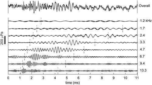
In each ½-octave frequency band, the root mean square (rms) noise was estimated for the analysis time-window from the difference between the two replicate waveforms. The TEOAE rms signal amplitude was then estimated using an unbiased estimator based on the mean of the two replicate waveforms, and the previously-estimated noise (e.g., Lineton 2013). The EHF TEOAE signal amplitude in the 8–16 kHz region was estimated by combining the signal power in the 9.4 and 13.3 kHz bands. The mean (standard deviation) of the signal amplitude was 6.2 dB SPL (8.0 dB), while the mean (standard deviation) of TEOAE signal-to-noise ratio was 5.9 dB (7.8 dB). As expected, there was a statistically significant negative correlation between band-averaged amplitudes of the EHF TEOAEs and EHF HTLs (Spearman’s rho = −0.49; p < 0.01). The ½-octave bands below 8 kHz were also calculated, but for descriptive purposes only, and did not feature in any further analysis. Box-and-whisker plots of the HTLs and TEOAE properties are shown in Figure 2.

Figure 2. Box and whisker plots the TEOAEs and HTLs across conventional and extended high-frequency regions. Boxes represent the interquartile range, with the median shown by a horizontal line. Circles indicate minor outliers, defined using fences 1.5 times the interquartile range. Whiskers represent the maximum and minimum values excluding outliers. (A) shows TEOAE amplitudes in ½-octave bands. Grey boxplots indicate centre frequencies used in calculating the EHF-TEOAE amplitude (i.e. 9.4 and 13.3 kHz); white boxplots indicate octave bands from 1.2 to 6.7 kHz which are used for descriptive purposes only. The TEOAEs at centre frequencies from 6.7 to 13.3 kHz denoted “HPF” were obtained using the high-pass filtered click stimulus; the other TEOAEs were those obtained using a conventional click stimulus. (B) shows the SNR of TEOAEs corresponding to the measurements described for (A). (C) shows the HTL at 10 frequencies; the grey boxplots indicate those values used to calculate the 6-frequency average EHF HTL, while the white boxes indicate the HTLs shown for descriptive purposes only.

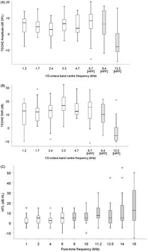
The boxplots (Figure 2(A)) indicate that the band-averaged EHF TEOAE amplitude in the 8–16 kHz range is dominated by the TEOAEs in the 8 to 11.3 kHz ½-octave band. This is expected for two reasons: first TEOAEs are known to reduce in amplitude as the evoking frequency increases, presumably due to middle-ear and cochlear physiology, and second, the calibration method is affected by a half-wave resonance, which will tend to emphasise components around 8 kHz (Charaziak and Shera 2017). Although these effects are expected to weaken the relationship under investigation between the AFS and TEOAE amplitudes, they do not invalidate the forthcoming correlational analysis (Section Test of relationship between AFS ripple depth, HTLs and TEOAE amplitude) because the absolute value of the TEOAE signal amplitude is not directly relevant to the study; only the correlation with ripple depth is of interest.

Another issue is that the TEOAE signal to noise ratio (SNR) is low for a considerable proportion of the measurements in the 11.3 to 16 kHz band, thereby making the corresponding estimate of the TEOAE amplitude unreliable. This does not invalidate the correlation analysis, and nor does it suggest that these individuals should be removed. This is because in cases where the SNR is low (e.g., ≤3dB), the unbiased estimate of the TEOAE amplitude will (in general) be very low in terms of dB SPL. This estimated low TEOAE amplitude, though not very accurate, still provides the useful information that this individual had TEOAEs that were much lower than the median in the sample. The correlational analysis in Section Test of relationship between AFS ripple depth, HTLs and TEOAE amplitude. used Spearman’s rank correlation which is robust to such errors.

3.1.2. Ripple depth of audiogram fine structure

In the following analyses, the stimulus level and HTL at all frequencies is expressed in interpolated dB HL values, based on an interpolation of the reference equivalent threshold sound pressure levels (RETSPLs) between the seven fixed frequencies in ISO 389-5 (2006) from 8 to 16 kHz.

The raw Bekesy track consists of a sawtooth-shaped plot of the hearing level of the stimulus tone, plotted against its frequency, with a turning point occurring at each button press and release. Features deemed artefactual were removed using the procedure reported in Kapadia and Lutman (1999). Briefly, turning-points were classed as ‘sore thumbs’ if they differed by ≥10 dB from both adjacent turning points of the same direction; pairs of turning points were classed as ‘glitches’ if they were ≤2 dB apart. In both cases, the turning points in this section were removed. The HTL was then defined as the mid-point between adjacent maxima and minima. The trace of HTL against frequency was then analysed in two ways to assess the magnitude of the spectral periodicity: the first used identification of peaks in the spectral domain (Section Processing of results); the second used a Fourier analysis to transform the audiogram into the “reciprocal spectral periodicity” domain (Section Test of relationship between AFS ripple depth, HTLs and TEOAE amplitude).

3.1.3. Depth of the ripple in the AFS in spectral domain

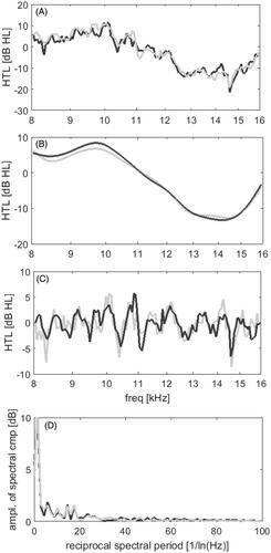
A metric for quantifying the depth of the audiogram ripple was performed based on the method proposed by Horst, Wit, and Albers (2003). In the present study, the HTL-vs-frequency function was first resampled to give equal logarithmic frequency intervals. It was then separated into two components based on their spectral periodicity: the audiogram coarse-structure and audiogram fine-structure (AFS) components (Figure 3). The audiogram coarse structure was obtained using a moving-average spectral filter over a frequency interval of 12.5%, thus smoothing out any spectral ripples with spacing f_C/Δf ≥ 8 which potential arose from cochlear standing waves; the resulting trace (Figure 3(B)) shows variations that may arise from phenomena such as ear-canal acoustic resonance. The AFS component was then calculated by subtracting the audiogram coarse structure from the total HTL-vs-frequency function; this was then used to assess the spectral ripple depth (Figure 3(C)). The AFS component was then smoothed to remove spectral ripples with spacing f_C/Δf ≥ 50, which were outside the spectral periodicity range of interest.

Figure 3. Example of two replicates of the Bekesy audiometry track for one participant (grey line: replicate 1; black line: replicate 2). (A) shows the total HTL-vs-frequency function. (B) shows the audiogram coarse structure obtained by the smoothing the trace in (A) using a moving-average filter with an averaging window in the logarithmic frequency domain coresponindg to 12.5% frequency interval (C) shows the audiogram fine-structure (AFS) obtained from the difference between the traces in (A,B). (D) show the reciprocal spectral periodicity distribution, obtained from of the Fourier series coefficients of the total HTL-vs-log frequency in (A). The values on the horizontal axis in (D) are equivalent to values of f_C/Δf.

The test-retest reliability of the two audiogram components was assessed from the correlation between the two replicates. The median (range) in the correlation for the audiogram coarse and fine-structure was 0.97 (0.81–1.0) and 0.6 (0.12–0.79) respectively. The two replicates were then averaged for further analysis.

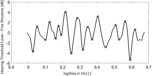
Cycles in the AFS were then identified from adjacent turning points that were separated by at least 1 dB (Figure 4). The amplitude in dB of each cycle was then calculated, and the average across the cycles was calculated as a metric for the mean ripple depth for each AFS.

Figure 4. An example of the average AFS of the two replicates with turning points extracted.

3.1.4. Ripple depth in the reciprocal spectral periodicity distribution

A second metric for quantifying the ripple depth was used based on Kapadia and Lutman (1999). The Fourier series coefficients of the HTL-vs-log-frequency function (Figure 3(A)) were calculated to convert from the log-frequency domain to the “reciprocal spectral periodicity” domain. The resulting distribution is plotted on a horizontal axis with units of [ln(Hz)]⁻¹ (Figure 3(D)). This unit corresponds to the previously used value of f_C/Δf, where f_C is the centre frequency, and Δf is the frequency spacing between adjacent ripple peaks; previous studies at conventional frequencies report values of f_C/Δf centred around 15 (e.g. Kapadia and Lutman 1999), while other studies suggest that the value increases somewhat with f_C from around 10 to 20 for values of f_C between 0.5 and 8 kHz (Shera 2003; Figure 3). Such features would show up in the reciprocal spectral periodicity domain as a peak located at a value between 10 and 20 [ln(Hz)]⁻¹ units.

For each participant, the average spectral ripple depth was quantified from the area under the distribution from 10 to 30 [ln(Hz)]⁻¹ in the reciprocal spectral periodicity domain. The range from 10 to 30 was chosen by extrapolating the trend seen in Shera (2003) up to 16 kHz.

3.2. Test of relationship between AFS ripple depth, HTLs and TEOAE amplitude

For both the above metrics of AFS ripple depth, two hypotheses were tested: (1) that the ripple depth be negatively correlated with the 6-frequency average HTL, and (2) be positively correlated with the band averaged EHF TEOAE amplitude. The Spearman correlation coefficient was calculated over the 28 participants and tested using a 2-tailed test for statistical significance, without correction for familywise error.

The AFS ripple depth metric calculated in the spectral domain (as in Horst, Wit, and Albers 2003) was found not to be statistically significantly correlated (p > 0.05) either with the 6-frequency average HTL (Spearman’s rho = 0.09), or with the band-averaged TEOAE amplitude (Spearman’s rho = 0.26).

The AFS ripple depth metric calculated in the reciprocal spectral periodicity domain (as in Kapadia and Lutman 1999) was also found not to be statistically significantly correlated with either the 6-frequency-average HTL or the band-averaged EHF TEOAE amplitude (Spearman’s rho = 0.22 and 0.16 respectively).

As expected, the two metrics of AFS ripple depth were positively correlated with each other (Spearman’s rho = 0.73, p < 0.01).

3.3. Exploring ripple characteristics of measured AFS

Visual inspection of the AFS appeared to show weaker and less regular spectral ripples than has been reported from lower frequency ranges. One way of characterising this is to examine the reciprocal spectral periodicity distribution of the AFS. At conventional frequencies, Kapadia and Lutman report a distinctive peak in this distribution in the periodicity range of 10 to 20 ln[Hz]⁻¹ when averaged across those individuals with detectable TEOAEs (Kapadia and Lutman 1999, Figure 2).

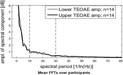
To explore whether any peak in the reciprocal spectral periodicity distribution was discernible in the EHF AFS data, average distributions across participants were calculated. The sample was first partitioned into two groups of 14 participants, depending on whether the average of EHF-TEOAEs was above or below the sample median. The average distribution across the 14 participants in both groups was then calculated. Unlike the distributions seen in the conventional frequency range (Kapadia and Lutman 1999), no discernible peak is visible in either distribution. There was also no clear difference in the two distributions (Figure 5).

Figure 5. The reciprocal spectral periodicity distribution averaged across individuals. Averages from two subgroups of the sample are plotted separately. Grey line is for the subgroup, n = 14 with the highest EHF TEOAEs averages. The black line is for the subgroup, n = 14 with lowest EHF TEOAEs averages.

It was also noticed that the mean ripple depth in the EHF region appeared lower than that found by previous studies at lower frequencies. The current study in the EHF range showed a mean ripple depth of 3.7 dB (1.7–7.1 dB) which was weaker than that in the previous studies, though this is a post-hoc observation.

3.4. SOAES

Over the frequency range from 8 to 16 kHz, few SOAEs were detected, and these were only weak in amplitude. With a threshold of 3 dB above the background noise level (estimated from adjacent frequency bins), only four participants exhibited clear SOAEs. The SOAEs were not analysed further. The participants exhibiting SOAEs were included in all the analyses.

4. Discussion

The results from the current study in the EHF region differ from those reported at lower frequencies in three respects. First, there is no distinctive peak seen in the reciprocal spectral periodicity distribution in the range of values of f_C/Δf from 10 to 30, unlike that seen in previous studies (Kapadia and Lutman 1999). This result differs from the findings of Kapadia and Lutman (1999) over the frequency range from 1.2 to 2.2, where individuals with weak TEOAEs showed weak audiogram ripple. Second, the mean ripple depth is lower than that found by previous studies at lower frequencies leading to poor test–retest reliability in some ears. Kapadia and Lutman (1999) reported ripple depths in the range of 2–12 dB while Horst, Wit, and Albers (2003) found a mean of about 6 dB (4–10 dB). The current study showed a mean of 3.7 dB (1.7–7.1 dB) which was weaker than that in the previous studies. Third, the lack of a significant correlation between the magnitude of the ripple depth and the frequency-average of either the HTLs or the TEOAE amplitude differs from the findings at lower frequencies (Horst et. al. 2003; Kapadia and Lutman 1999). This non-signficant result differs from the results of Horst, Wit, and Albers (2003; Figure 3) who found a significant correlation between the mean ripple depth and the frequency-average HTL over the range of 0.25–3.5 kHz.

These findings are unexpected from predictions from current theories of cochlear mechanics, in which both audiogram ripple and TEOAEs arise when there is both active amplification of the travelling wave and multiple reflections of the travelling wave between apical and basal sites. The apical site is thought to be due to inhomogeneities on the basilar membrane near the characteristic place of the stimulus frequency and the basal site due to the stapes (Zweig and Shera 1995; Talmadge et al. 1998; Wilson 1980a). The theory also predicts a minimum spectral ripple spacing, which is expected to lead to a peak in the reciprocal spectral periodicity (f_C/Δf) between 10 and 30 (Zweig and Shera 1995; Talmadge et al. 1998, Shera 2003). Support for the applicability of this theory at frequencies up to 13.9 kHz is seen in the relationship between SOAEs and audiogram ripple locations reported by Baiduc, Lee, and Dhar (2014).

We consider here possible explanations for the findings of the current results within the cochlear mechanical theory outlined above. The relatively weaker ripple pattern at EHFs relative to conventional frequencies and the lack of any discernible peak in the reciprocal spectral periodicity distribution (Figure 3) may have several causes. The generation of audiogram ripple requires several different elements: inhomogeneities arising from longitudinal spatial variation in the wave-impedance along the basilar membrane, coherent scattering of the travelling wave from these inhomogeneities, active amplification of the travelling wave to give a “tall-and-broad” travelling wave envelope (Zweig and Shera 1995), and basal reflection from the stapes. Thus the weaker AFS ripple pattern seen in higher-frequency regions may arise from a lower cochlear amplifier gain, from less potent inhomogeneities, or potentially from a different interaction between the travelling wave and the inhomogeneities, perhaps due to differences in cochlear mechanical properties. Measurements of SFOAEs by Shera (2003; Figure 3) suggest that the travelling wave envelope becomes increasingly sharply tuned as the frequency is increased up to 7 kHz, which may be due to increasing cochlear amplifier gain. If this trend continues to the 8–16 kHz region, then we might expect greater cochlear amplifier gain, and hence a stronger AFS ripple pattern, leading to a greater amplitude in the reciprocal spectral periodicity distribution. There is, however, a complication: increasing the cochlear amplifier gain also leads to a narrower travelling wave envelope, which leads to reflections being less coherent (Zweig and Shera 1995). The consequence is that as the travelling wave envelope becomes narrower, any peak in the reciprocal spectral periodicity distribution is expected to become broader leading to less coherent scattering (Zweig and Shera 1995). A consequence of this is that the peak in the reciprocal spectral periodicity distribution may become less distinct as it comprises a broader range of spectral periods. A further possibility is that the interference pattern breaks down in the basal cochlear region as the peak in the travelling wave becomes located closer to the stapes, giving a restricted region in which the travelling wave can develop. However, simulations by Ku, Elliott, and Lineton (2008) using a cochlear model which incorporates the main elements of the cochlear mechanical theory, predicted cochlear standing waves (which would generate an AFS ripple pattern) in the basal, EHF region, thus suggesting that there is no inherent theoretical barrier to producing AFS ripple in the basal region.

The weaker AFS ripple pattern described above is one possible reason why no significant correlation between ripple depth and the frequency-averaged HTL and TEOAE metrics was found in the current study; the measured ripple depth will be more contaminated by measurement errors in the EHF region than at lower frequencies. Another possible reason for the lack of correlation may be that intersubject variability in EHF-HTLs is much greater than that at conventional frequencies (Bharadwaj et al. 2019; Ahmed et al. 2001; Souza et al. 2014). This is possibly due to reasons that are not associated with cochlear activity, but rather with differences in transmission through the outer and middle ears which would not affect ripple depth, but would affect frequency-averaged metrics. The outer ear is known to lead to greater intersubject variability in HTLs due in part to standing waves in the ear canal (Souza et al. 2014). Transmission through the middle ear may also be a source of greater intersubject variability: the transmissibility reduces rapidly with increasing frequency, meaning that small intersubject differences in the frequency of the “knee-point” in transmission may lead to large intersubject differences in HTL. If this were the case, then the intersubject variability due to middle ear properties would be greater in the EHF region than at lower frequencies. As these additional sources of variability in the frequency-averaged HTL in the EHF region are unrelated to the ripple depth, they could explain why any correlation between HTL amplitude and ripple depth is weaker in the EHF-region than the conventional range. Similar arguments relate to TEOAE amplitudes, which are affected both by forward and reverse transmission through the middle ear. The measured band-averaged TEOAE amplitude is likely to be dominated by components at the lower end of the frequency range (Figure 2). The SNR of the EHF TEOAEs were also reduced at higher frequencies, leading to greater errors in the estimated TEOAE amplitude. Finally, the studies of Kapadia and Lutman (1999) and Horst, Wit, and Albers (2003) both selected participant groups that maximised the correlations seen at lower frequencies, while the current studies relied on intersubject variability in a sample drawn from a more homogeneous population. In summary, there are several possible reasons for the weaker AFS ripple pattern and lack of correlations, but no single obvious explanation.

5. Conclusions

Previous studies in the conventional frequency range have shown that there is a link between spectral periodicity in the audiogram and overall amplitudes of both TEOAEs and HTLs. The present study aimed to evaluate whether there was a similar link observed in the EHF region (8–16 kHz). In contrast to the findings in the conventional frequency range, in the EHF region, no significant correlation was found between the AFS ripple depth and the frequency-averaged amplitudes of either TEOAEs and HTLs. Additionally, AFS ripple depth was weaker in in the EHF region, and there was no distinctive peak noticed in the distribution of spectral periods. Several possible explanations due to cochlear mechanical properties are discussed.

Disclosure statement

No potential conflict of interest was reported by the author(s).

Additional information

Funding

This work was supported by King Saud University, Riyadh, Saudi Arabia and Institute of Sound and Vibration Research, University of Southampton, UK.

References

- Ahmed, H. O., J. H. Dennis, O. Badran, M. Ismail, S. G. Ballal, A. Ashoor, and D. Jerwood. 2001. “High-Frequency (10-18 kHz) Hearing Thresholds: reliability, and Effects of Age and Occupational Noise Exposure.” Occupational Medicine 51 (4): 245–258. doi:https://doi.org/10.1093/occmed/51.4.245.
- Baiduc, R. R., J. Lee, and J. Dhar. 2014. “Spontaneous Otoacoustic Emissions, Threshold Microstructure, and Psychophysical Tuning over a Wide Frequency Range in Humans.” Journal of the Acoustical Society of America 135 (1): 300–314. doi:https://doi.org/10.1121/1.4840775.
- Bharadwaj, H. M., A. R. Mai, J. M. Simpson, I. Choi, M. G. Heinz, and B. G. Shinn-Cunningham. 2019. “Non-Invasive Assays of Cochlear Synaptopathy – Candidates and Considerations.” Neuroscience 407: 53–66. doi:https://doi.org/10.1016/j.neuroscience.2019.02.031.
- BSA 2011. “Recommended Procedure; Pure-Tone Air-Conduction and Bone-Conduction Threshold Audiometry With and Without Masking.” British Society of Audiology.
- Charaziak, K. K., and C. A. Shera. 2017. “Compensating for Ear-Canal Acoustics When Measuring Otoacoustic Emissions.” The Journal of the Acoustical Society of America 141 (1): 515–531. doi:https://doi.org/10.1121/1.4973618.
- Dallmayr, C. 1987. “Stationary and Dynamical Properties of Simultaneous Evoked Otoacoustic Emissions (SEOAE) Acustica.” Acta Acustica united with Acustica 63: 223–255.
- Dewey, J. B., and S. Dhar. 2017. “A Common Microstructure in Behavioral Hearing Thresholds and Stimulus-Frequency Otoacoustic Emissions.” The Journal of the Acoustical Society of America 142 (5): 3069 doi:https://doi.org/10.1121/1.5009562.
- Elliott, E. 1958. “A Ripple Effect in the audiogram.” Nature 181 (4615): 1076. doi:https://doi.org/10.1038/1811076a0.
- Goodman, S. S., D. F. Fitzpatrick, J. C. Ellison, W. Jesteadt, and D. H. Keefe. 2009. “High-Frequency Click-Evoked Otoacoustic Emissions and Behavioral Thresholds in Humans.” The Journal of the Acoustical Society of America 125 (2): 1014–1032. doi:https://doi.org/10.1121/1.3056566.
- Horst, J. W., H. P. Wit, and F. W. J. Albers. 2003. “Quantification of Audiogram Fine-Structure as a Function of Hearing Threshold.” Hearing Research 176 (1-2): 105–112. doi:https://doi.org/10.1016/s0378-5955(02)00749-9.
- IEC 60318-1 1998. Electroacoustics - Simulator of human head and ear; part 1- Ear simulator for the calibration of supra-aural earphones, International Electrotechnical Commission.
- IEC 60318-4 2010. Electroacoustics – Simulators of human head and ear; part 4 – occluded ear simulator for the measurement of earphones coupled to the ear by means of ear inserts, International Electrotechnical Commission.
- ISO 389-5. 2006. Acoustics – Reference zero for the calibration of audiometric equipment. Part 5: Reference equivalent threshold sound pressure levels for pure tones in the frequency range 8 kHz to 16 kHz, International Organization for Standardization.
- ISO 28961. 2012. Acoustics. Statistical Distribution of Hearing Thresholds of Otologically Normal Persons in the Age Range from 18 Years to 25 Years Under Free-Field Listening Conditions, International Organization for Standardization.
- ISO 389-7. 2019. Acoustics – Reference zero for the calibration of audiometric equipment Part 7: Reference threshold of hearing under free field and diffuse-field listening conditions International Organization for Standardization.
- Kapadia, S., and M. E. Lutman. 1999. “Reduced ‘Audiogram Ripple' in Normally-Hearing Subjects with Weak Otoacoustic Emissions.” Audiology 38 (5): 257–261. doi:https://doi.org/10.3109/00206099909073031.
- Keefe, D. H. 1998. “Double-Evoked Otoacoustic Emissions. I. Measurement Theory and Nonlinear Coherence.” Journal of the Acoustical Society of America. 103 (6): 3489–3498. doi:https://doi.org/10.1121/1.423057.
- Kemp, D. T. 1979. “The Evoked Cochlear Mechanical Response and the Auditory Microstructure - Evidence for a New Element in Cochlear Mechanics” Scandinavian Audiology Supplementum 9: 35–47.
- Ku, E. M., S. J. Elliott, and B. Lineton. 2008. “Statistics of Instabilities in a State Space Model of the Human Cochlea.” Journal of the Acoustical Society of America 124 (2): 1068–1079. doi:https://doi.org/10.1121/1.2939133.
- Lee, J., S. Dhar, R. Abel, R. Banakis, and E. Grolley. 2012. “Behavioral Hearing Thresholds between 0.125 and 20 kHz Using Depth-Compensated Ear Simulator Calibration.” Ear Hear 3: 315–329.
- Leijon, A. 1992. “Quantization Error in Clinical Pure-Tone Audiometry.” Scandinavian Audiology 21 (2): 103–108. doi:https://doi.org/10.3109/01050399209045989.
- Lineton, B. 2013. “Theoretical Analysis of Signal-to-Noise Ratios for Transient Evoked Otoacoustic Emission Recordings.” The Journal of the Acoustical Society of America 134 (3): 2118–2126. doi:https://doi.org/10.1121/1.4816493.
- Long, G. R. 1984. “The Microstructure of Quiet and Masked Thresholds.” Hearing Research 15 (1): 73–87. doi:https://doi.org/10.1016/0378-5955(84)90227-2.
- Long, G. R., and A. Tubis. 1988. “Investigation into the Nature of the Association between Threshold Microstructure and Otoacoustic Emissions.” Hearing Research 36 (2-3): 125–138. doi:https://doi.org/10.1016/0378-5955(88)90055-X.
- Lutman, M. E., and J. Deeks. 1999. “Correspondence Amongst Microstructure Patterns Observed in Otoacoustic Emissions and Békésy audiometry.” Audiology 38 (5): 263–266. doi:https://doi.org/10.3109/00206099909073032.
- Moller, H., M. F. Sorensen, D. Hammershoi, and C. B. Jensen. 1995. “Head-Related Transfer Functions of Human Subjects.” Journal of the Audio Engineering Society 43: 300–320.
- Probst, R., A. C. Coats, G. K. Martin, and B. L. Lonsbury Martin. 1986. “Spontaneous, Click-, and Tone Burst-Evoked Otoacoustic Emissions from Normal Ears.” Hearing Research 21 (3): 261–275. doi:https://doi.org/10.1016/0378-5955(86)90224-8.
- Puria, Sunil. 2003. “Measurements of Human Middle Ear Forward and Reverse Acoustics: Implications for Otoacoustic Emissions.” The Journal of the Acoustical Society of America 113 (5): 2773–2789. doi:https://doi.org/10.1121/1.1564018.
- Rodríguez Valiente, A., A. Trinidad, J. García Berrocal, C. Górriz, and R. Ramírez Camacho. 2014. “Extended high-frequency (9-20 kHz) audiometry reference thresholds in 645 healthy subjects.” International Journal of Audiology 53 (8): 531–545. doi:https://doi.org/10.3109/14992027.2014.893375.
- Schmuziger, N., R. Probst, and J. Smurzynski. 2005. “Otoacoustic Emissions and Extended High-Frequency Hearing Sensitivity in Young Adults Emisiones Otoacústicas y Sensibilidad Extendida a Frecuencias Altas en Adultos Jóvenes.” International Journal of Audiology 44 (1): 24–30. doi:https://doi.org/10.1080/14992020400022660.
- Schloth, E. 1983. “Relation between Spectral Composition of Spontaneous Otoacoustic Emissions and Fine-Structure of Threshold in Quiet.” Acustica 53: 252–256.
- Shera, C. A., J. J. Guinan, and A. J. Oxenham. 2002. “Revised Estimates of Human Cochlear Tuning from Otoacoustic and Behavioral Measurements.” Proceedings of the National Academy of Sciences of the United States of America 99 (5): 3318–2232. doi:https://doi.org/10.1073/pnas.032675099
- Shera, C. A. 2003. “Mammalian Spontaneous Otoacoustic Emissions Are Amplitude-Stabilized Cochlear Standing Waves.” The Journal of the Acoustical Society of America 114 (1): 244–262. doi:https://doi.org/10.1121/1.1575750
- Shera, C. A., and J. J. Guinan. 2003. “Stimulus-Frequency-Emission Group Delay: A Test of Coherent Reflection Filtering and a Window on Cochlear Tuning.” The Journal of the Acoustical Society of America 113 (5): 2762–2772. doi:https://doi.org/10.1121/1.1557211.
- Siegel, J. H. 1994. “Ear-Canal Standing Waves and High-Frequency Sound Calibration Using Otoacoustic Emission Probes.” Journal of the Acoustical Society of America 95 (5): 2589–2597. doi:https://doi.org/10.1121/1.409829.
- Souza, N. N., S. Dhar, S. T. Neely, and J. H. Siegel. 2014. “Comparison of Nine Methods to Estimate Ear-Canal Stimulus Levels.” The Journal of the Acoustical Society of America 136 (4): 1768–1787. doi:https://doi.org/10.1121/1.4894787.
- Talmadge, C. L., and A. Tubis. 1993. “On Modelling the Connection between Spontaneous and Evoked Otoacoustic Emissions.” In Biophysics of Hair-Cell Sensory Systems, edited by H. Duifhuis, J.W. Horst, P. van Dijk, S.M. van Netten, 25–32. Singapore: World Scientific.
- Talmadge, C. L., A. Tubis, G. R. Long, and P. Piskorski. 1998. “Modeling Otoacoustic Emission and Hearing Threshold Fine Structures.” The Journal of the Acoustical Society of America 104 (3 Pt 1): 1517–1543. doi:https://doi.org/10.1121/1.424364
- Thomas, I. B. 1975. “Microstructure of the Pure-Tone Threshold.” Journal of the Acoustical Society of America 57 (S1): S26–S27. doi:https://doi.org/10.1121/1.1995148.
- Wilson, J. P. 1980. “Evidence for a Cochlear Origin for Acoustic Re-Emissions, Threshold Fine-Structure and Tonal Tinnitus.” Hearing Research 2 (3-4): 233–252. doi:https://doi.org/10.1016/0378-5955(80)90060-X.
- Yasin, I., and C. J. Plack. 2005. “Psychophysical Tuning Curves at Very High Frequencies.” The Journal of the Acoustical Society of America 118 (4): 2498–2506. doi:https://doi.org/10.1121/1.2035594.
- Zweig, G., and C. A. Shera. 1995. “The Origin of Periodicity in the Spectrum of Evoked Otoacoustic Emissions.” The Journal of the Acoustical Society of America 98 (4): 2018–2047. doi:https://doi.org/10.1121/1.413320.
- Zwicker, E., and E. Schloth. 1984. “Interrelation of Different oto-acoustic emissions.” The Journal of the Acoustical Society of America 75 (4): 1148–1154. doi:https://doi.org/10.1121/1.390763.