Non-negative matrix factorization improves the efficiency of recording frequency-following responses in normal-hearing adults and neonates

Abstract

Objective

One challenge in extracting the scalp-recorded frequency-following response (FFR) is related to its inherently small amplitude, which means that the response cannot be identified with confidence when only a relatively small number of recording sweeps are included in the averaging procedure.

Design

This study examined how the non-negative matrix factorisation (NMF) algorithm with a source separation constraint could be applied to improve the efficiency of FFR recordings. Conventional FFRs elicited by an English vowel/i/with a rising frequency contour were collected. Study sample: Fifteen normal-hearing adults and 15 normal-hearing neonates were recruited.

Results

The improvements of FFR recordings, defined as the correlation coefficient and root-mean-square differences across a sweep series of amplitude spectrograms before and after the application of the source separation NMF (SSNMF) algorithm, were characterised through an exponential curve fitting model. Statistical analysis of variance indicated that the SSNMF algorithm was able to enhance the FFRs recorded in both groups of participants.

Conclusions

Such improvements enabled FFR extractions in a relatively small number of recording sweeps, and opened a new window to better understand how speech sounds are processed in the human brain.

KEYWORDS

Keywords:

• Electrophysiology
• pediatric
• non-negative matrix factorization
• frequency-following response

1. Introduction

The scalp-recorded frequency-following response (FFR) is an electroencephalographic (EEG) measurement that has been widely used to evaluate how the human brain perceives and tracks changes in the fundamental frequency (F0) and its harmonics with periodic speech stimulations (Hart and Jeng 2021; Skoe and Kraus 2010). For example, the FFR has been utilised to investigate how pitch related information is processed in normal-hearing adults (Jeng et al. 2011; Jeng et al. 2018; Krishnan et al. 2004) and neonates (Jeng, Lin, and Wang 2016; Musacchia et al. 2020; Ribas-Prats et al. 2019; Van Dyke et al. 2017). The FFR is also useful in assessing pitch-processing deficits for people with dyslexia (Chandrasekaran et al. 2009; Hornickel and Kraus 2013), autism spectrum disorders (Font-Alaminos et al. 2020; Russo et al. 2008), and concussions (Kraus et al. 2017; Kraus et al. 2016; Rauterkus et al. 2021).

Despite the usefulness of the FFR, one major challenge still exists. This challenge is related to the negative influences of different kinds of noise that are embedded in a recording (Li and Jeng 2011). Because the FFR is a small-amplitude response (usually ≤ 100 nV) (Jeng et al. 2011; Skoe and Kraus 2010), any kind of noise, either environmental or physiological in nature, may have substantial and adverse effects on the signal-to-noise ratio of a recording. Although eliminating noise from its source may be the optimal solution, it is not always possible. Signal averaging is a traditional method that is commonly used to reduce noise in an FFR recording. As noise tends to be random, the total sum of noise can be reduced by including a sufficient number of recording sweeps in the averaging procedure. The conventional averaging procedure has been used successfully when a relatively large number of recording sweeps (e.g. 4000 sweeps) are included. When only a relatively small number of recording sweeps (e.g. 500 sweeps) are included in the averaging procedure, it is usually unable to extract a visually identifiable FFR (Skoe and Kraus 2010).

The number of sweeps needed to obtain a visually identifiable FFR represents a challenge for participants who cannot stay quiet for an extended period of time. This challenge becomes unneglectable when recording FFRs from neonates in the maternity ward of a hospital, where excessive electromagnetic interference and the short sleep span of neonates may force a recording to stop prematurely. When recording FFRs, time is of utmost importance. The goal of this study is to develop an algorithm that can be used to improve the efficiency of FFR recordings, therefore reducing the number of sweeps needed to detect the presence of an FFR.

To improve the detectability of an FFR, several machine learning algorithms have been applied in recent years (Hart and Jeng 2021; Llanos, Xie, and Chandrasekaran 2017; Xie, Reetzke, and Chandrasekaran 2018; Xie, Reetzke, and Chandrasekaran 2019; Yi et al. 2017; Hart and Jeng 2018). For example, Llanos and colleagues used a hidden Markov algorithm to classify FFR recordings in response to four different Mandarin tones (Llanos, Xie, and Chandrasekaran 2017). Xie and colleagues adopted a modified Support Vector Machine algorithm (Xie, Reetzke, and Chandrasekaran 2019), based on a series of spectral features that were predetermined from speech samples of 20 native Mandarin speakers, to map FFR recordings into three different pitch patterns. Hart and Jeng reported the usefulness of 23 supervised machine learning algorithms in detecting the presence or absence of an FFR for recordings that were obtained in 1–3 day old neonates (Hart and Jeng 2021). Although all the aforementioned machine learning algorithms have shown variable success in mapping FFR recordings into different categories, all of them are supervised algorithms. This means that the experimenter will have to provide a predetermined “gold standard” for each recording, which is often unavailable. Furthermore, none of the above-mentioned algorithms can actually enhance the visibility of an FFR nor reduce the amount of noise in a recording.

The non-negative matrix factorisation (NMF), first reported by Lee and Seung (Lee and Seung 1999), is a machine learning algorithm for extracting parts-based representations (i.e. separating different components of a mixture). It has been widely used in the enhancement of speech and wildlife vocalizations (Smaragdis et al. 2014; Lin and Tsao 2020; Lin, Akamatsu, and Tsao 2021b). Unlike most of the machine learning algorithms that generate categorical outputs, the NMF algorithm can discover interpretable components that are associated with the spectral and temporal features of sound sources, and thus overcomes a major challenge in source separation. Conventional approaches of NMF-based source separation require a clean signal for learning source-specific features. After performing this supervised training procedure on the target sound and noise, the NMF algorithm can be employed to predict their relative contributions and perform source reconstruction. Despite that, preparing clean recordings for supervised training is challenging for the analysis of FFR.

In this study, we developed a new source separation NMF (SSNMF) algorithm that does not require any supervised training by integrating a source separation constraint (i.e. a rule dictating how each component is computed) in the conventional NMF algorithm. We applied the SSNMF algorithm on EEG recordings that were obtained from normal-hearing adults and neonates and evaluated the algorithm performance in improving the efficiency of FFR recordings. Based on the extraction results, we discussed potential applications of the SSNMF algorithm in FFR research.

2. Method

2.1. Participant information

Fifteen American adults (10 females and 5 males, 20–33 years old) were recruited from Ohio University in Athens, Ohio and its nearby communities. All adult participants had normal hearing as determined by audiometric hearing thresholds ≤ 20 dB HL at octave frequencies between 250 and 8000 Hz. All recordings of adult participants were obtained in an acoustically treated sound booth in the Auditory Electrophysiology Laboratory at Ohio University.

To examine the effectiveness of the SSNMF algorithm for participants during their immediate postnatal days, 15 American neonates (6 girls and 9 boys, 1–3 days after birth) were also recruited. All neonates were born to native English speakers at OhioHealth O’Bleness Hospital in Athens, Ohio. Neonatal participants completed the mandatory Universal Newborn Hearing Screening and received passing results through distortion-product otoacoustic emissions or automated auditory brainstem responses. Parents of all neonates gave written consent. All recordings were obtained in a quiet room at the hospital when the neonates were asleep or resting in a bassinette. All research protocols and experimental procedures were approved by the Institutional Review Boards at Ohio University and OhioHealth O’Bleness Hospital.

2.2. Stimulus presentation

An English vowel/i/with a rising frequency contour (F0 ranging from 102 to 140 Hz) was utilised to evoke scalp-recorded frequency-following responses. This stimulus had a duration of 150 ms with a cosine-square rising and falling ramp of 10 ms. The stimulus was delivered through a 16-bit digital-to-analog converter (National Instruments USB-6216), a portable audiometer with an adjustable attenuator (Maico MA 42), and an electromagnetically shielded insert earphone (Etymotic ER-3A). The stimulus was delivered monaurally to the right ear via foamed ear tips (Etymotic ER3-14A) for adult participants and circum-aural earcups (ALGO Flexicoupler) for neonatal participants. The stimulus was presented at 70 dB SPL for adult participants and, to compensate a 5 dB real-ear-to-coupler difference, 65 dB SPL for neonatal participants (Jeng et al. 2011). The stimulus was calibrated using a sound level metre (Larson Davis 824, flat weighting) and a 2 c.c. coupler (G.R.A.S. RA0038). The silent interval between the offset of a stimulus and the onset of the next one was set at 45 ms. The stimulus was presented a total of 8800 times. This resulted in a recording time of approximately 28.6 minutes (195 ms × 8800 = 28.6 minutes) for each participant.

2.3. Recording parameters

Continuous brainwaves were recorded via three gold-plated recording electrodes that were placed on the high forehead (non-inverting), right mastoid (inverting), and left mastoid (ground) for adult participants. For neonates, three snap-on recording electrodes (Ambu Neuroline 720) were montaged on the high forehead and both mastoids. All electrode impedances were kept under 5000 ohms. Recorded brainwaves were amplified (Intelligent Hearing Systems Opt-Amp 8002, gain 50,000), bandpass filtered (10–3000 Hz, 6 dB/octave), digitally sampled (National Instruments USB-6216, 16-bit resolution, 20,000 samples/s), and saved on a computer for offline analysis. Alternating stimulus polarities were used to minimise possible contaminations of stimulus artefact and cochlear microphonic. All stimulus presentations, trigger synchronisations, and recording parameters were controlled by using custom-built software written in LabVIEW (National Instruments, Austin, TX).

2.4. Data analysis

To better isolate spectral energies at the F0 contour and its harmonics, continuous brainwaves were filtered through a digital Butterworth filter (90–1500 Hz, 24 dB/octave, zero-phase shift). Filtered brainwaves were segmented into sweeps of 195 ms in length (150 ms stimulus duration + 45 ms silent interval). Any sweeps containing a voltage larger than ±25 µV were removed. The first 8000 accepted sweeps were included for the subsequent analyses.

To evaluate the effectiveness of the SSNMF algorithm as a function of the number of sweeps, distinct sweep numbers were included in the averaging procedure. All sweeps were randomly selected from a pool of the 8000 accepted sweeps. The numbers of sweeps used in the averaging procedure were 100, 250, 500, 1000, 2000, 3000, 4000, 5000, 6000, 7000, and 8000 sweeps. This resulted in a total of 11 nSweep conditions to be analysed. The averaged time waveform of each nSweep condition was converted to an amplitude spectrogram by using a narrow-band sliding-window spectrogram (window size 50 ms, step size 0.5 ms, frequency resolution 1 Hz, Hanning windowing). The first 201 windowed time bins of each amplitude spectrogram (that corresponded to the 150 ms duration of the stimulus presentation) were flattened into a vector, and the vectors of the 11 nSweep conditions were subsequently concatenated as input signals in the SSNMF algorithm.

2.5. Design of a source separation algorithm

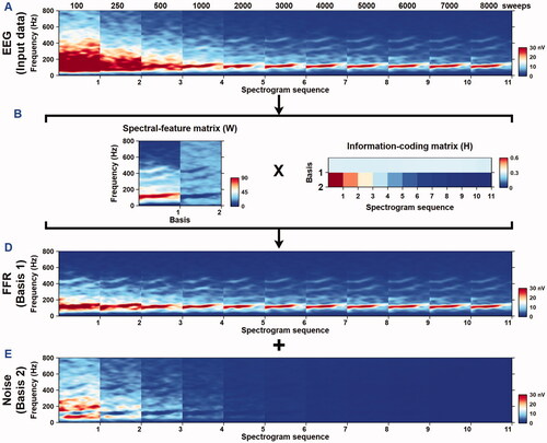
The SSNMF algorithm was based on two assumptions: (1) each EEG recording was a mixture of FFR and noise, and (2) an FFR was present with similar magnitudes in each recording sweep. Based on the first assumption, the SSNMF algorithm was designed to learn two spectral bases: one for the targeted FFR and another for noise. The SSNMF algorithm included several steps of signal processing and iteration cycles (Figure 1).

Figure 1. Design of a source separation NMF algorithm.

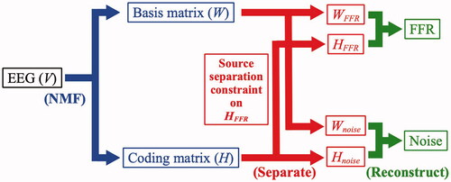
Specifically, the first assumption was integrated in the conventional NMF algorithm (Figure 1 items marked in blue) (Lee and Seung 1999) – a machine learning model that learned and factorised a non-negative input matrix (V) into two non-negative matrices: spectral-basis matrix (W) and information-coding matrix (H), by using the formula: (1) $$V_{\mathit{ij}}\approx {\left(\mathit{WH}\right)}_{\mathit{ij}}={\sum }_{k=1}^n{W}_{\mathit{ik}}{H}_{\mathit{kj}}$$(1) where i and j denoted elements along the first (a flattened vector of frequency × time) and second (a series of amplitude spectrograms) dimensions of a matrix, respectively; and k annotated the k-th basis from a total of n bases.

The non-negative constraint of the matrices V, W, and H, ensured that the matrices W and H could learn parts-based representation that were essential to reconstruct the data, as demonstrated in various applications of the NMF algorithm in audio source separations (Smaragdis et al. 2014; Lin and Tsao 2020). Such constraint reinforced the idea that the input data was a linear sum of multiple sources, and thus reflected the additive nature of EEG recordings.

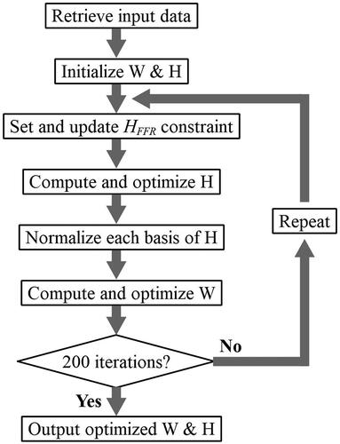
The matrices W and H were initialised with random values and subsequently updated by using the standard NMF multiplicative update rule (Lee and Seung 1999). The second assumption was implemented through a source separation constraint (Figure 1 items marked in red) (Lin, Akamatsu, and Tsao 2021b). Specifically, in the beginning of each iteration, the first basis of the information-coding matrix H (i.e. H_FFR) was set to be invariant (among the amplitude spectrograms produced in the 11 nSweep conditions) by calculating an average across the entire H_FFR vector. This constraint forced the two bases of the spectral-basis matrix W (i.e. W_FFR and W_noise) to learn and separate the spectral features of the FFR and noise, respectively. After 200 iterations (Lin, Fang, and Tsao 2017), the FFR and noise were reconstructed (Figure 1 items marked in green) separately by multiplying the input data matrix V to their corresponding W-H ratios, by using the formulae: (2) $$\mathit{FFR}=V\circ \left(W_{\mathit{FFR}}{H}_{\mathit{FFR}}/\mathit{WH}\right)$$(2) (3) $$\mathit{Noise}=V\circ \left(W_{\mathit{noise}}{H}_{\mathit{noise}}/WH\right)$$(3)

2.6. Evaluation of the algorithm performance

For each participant, amplitude spectrograms obtained in the 11 nSweep conditions were concatenated to form a sweep series of spectrograms. Following previous works of the NMF-based source separation (Lin, Fang, and Tsao 2017; Heard et al. 2021; Lin et al. 2021a), amplitude spectrograms were transformed to a log scale during optimisation. To ensure that the SSNMF algorithm converged to a stable learning result, each decomposition went through a total of 200 optimisation cycles before the spectral-basis and information-coding matrices were finalised (Lin, Fang, and Tsao 2017). For clarity, Figure 2 shows the basic procedural steps that were involved in an iteration cycle to fine tune the output matrices. The resultant matrices were used jointly to construct the amplitude spectrograms of the targeted FFR and residual noise.

Figure 2. Procedural steps of an iteration cycle.

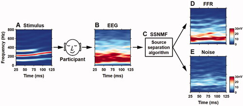
Narrow-band sliding-window spectrograms (window size 50 ms, step size 0.5 ms, frequency resolution 1 Hz) were utilised to visualise the effects of source separation. Figure 3 shows the amplitude spectrogram of the stimulus (Figure 3A), grand-averaged spectrogram obtained at 500 sweeps before the SSNMF decomposition (Figure 3B), SSNMF components (Figure 3C), grand-averaged spectrogram of the targeted FFR separated by using the SSNMF algorithm (Figure 3D), and grand-averaged spectrogram of the noise (Figure 3E) extracted by using the SSNMF algorithm. Spectral energies following the stimulus F0 contour and its harmonics were enhanced in the targeted FFR spectrogram, likely due to the fact that a substantial amount of noise was removed through the SSNMF decomposition. This example displayed grand-averaged spectrograms that were obtained in the adult participants at 500 sweeps.

Figure 3. A typical example of the SSNMF decomposition. These grand-averaged spectrograms were obtained from fifteen adult participants when the 500 sweeps were included in the averaging procedure.

Before the effectiveness of the SSNMF algorithm could be determined, the following two procedures must be evaluated: (1) effects of the conventional averaging (AVG) procedure and (2) effects of the conventional averaging plus SSNMF (AVG + SSNMF) procedure. Two objective measurements, Correlation Coefficient (CC) and Root-Mean-Square Error (RMSE), were administered to estimate the overall correlation and amplitude deviation between the AVG and AVG + SSNMF procedures. For consistency, when computing a CC or RMSE value, the amplitude spectrogram derived from the 8000 accepted sweeps that did not go through the SSNMF algorithm was used as a reference. Specifically, the CC measurement quantified the extent in which the extracted FFR spectrogram of each nSweep condition correlated with the amplitude spectrogram of the reference. When computing a CC value, spectrogram amplitudes were Z transformed (i.e. subtracted the sample mean and standardised to one standard deviation). The resultant CC values fell into a range between 0 (no correlation) and 1 (perfect correlation). The RMSE measurement represented the extent in which the amplitude spectrogram of each nSweep condition differed from the amplitude spectrogram of the reference. The same principle was applied in both the AVG and AVG + SSNMF procedures for all recordings obtained in adult and neonatal participants.

For the effects of the AVG procedure, CC was computed by performing a cross correlation between the amplitude spectrogram that did not go through the SSNMF algorithm for each nSweep condition and the amplitude spectrogram of the 8000-sweep reference recording. The resultant correlation coefficient was defined as the CC value for that nSweep condition. The RMSE value was calculated by subtracting the amplitude spectrogram that did not go through the SSNMF algorithm for each nSweep condition from the amplitude spectrogram of the reference recording. The root-mean-square value of the difference spectrogram was defined as the RMSE value for that nSweep condition.

For the effects of the AVG + SSNMF procedure, CC was computed by performing a cross correlation between the amplitude spectrogram derived from the SSNMF algorithm for each nSweep condition and the amplitude spectrogram of the 8000-sweep reference recording. The resultant correlation coefficient was defined as the CC value for that nSweep condition. RMSE was calculated by subtracting the amplitude spectrogram derived from the SSNMF algorithm for each nSweep condition from the amplitude spectrogram of the reference recording. The root-mean-square value of the difference spectrogram was defined as the RMSE value for that nSweep condition.

The performance of the SSNMF algorithm was computed by subtracting the effects of the AVG procedure from those of the AVG + SSNMF procedure. Two performance indices, FFR Enhancement and Noise Reduction, were used to quantify the effectiveness of the SSNMF algorithm. Specifically, FFR Enhancement was computed by subtracting the CC value of the AVG procedure from that of the AVG + SSNMF procedure. Noise Reduction was calculated by subtracting the RMSE value of the AVG procedure from that of the AVG + SSNMF procedure. For clarity, the SSNMF algorithm written in the Python programming language and a sample recording are available on the first author’s (FCJ) GitHub repository https://github.com/fjeng/ffr_ssnmf_feasibility.

2.7. Exponential modeling of improvements in FFR recordings

To delineate the improvement of efficiency in FFR recordings (i.e. performance of the SSNMF algorithm), an exponential curve fitting model was utilised. For FFR Enhancement that followed a descending trend with increasing number of sweeps, the following model was used to determine the dependency of SSNMF performance on the number of sweeps included in each recording: (4) $$A\left(n\right)=A_{AS}\left(e^{-\frac{n}{\tau }}\right)+A_{DC}$$(4) where A represented the performance index (FFR Enhancement); A_AS indicated the asymptotic amplitude of the fitted curve, excluding the direct current component; n was the number of sweeps included in each recording; e represented the Euler’s mathematical constant = 2.7182; τ indicated the time constant of the fitted curve (i.e. the number of sweeps required to reach 63% of the asymptotic amplitude), and A_DC denoted the direct current component of the fitted curve (i.e. the overall elevation of the fitted curve). For Noise Reduction that followed an ascending trend with increasing number of sweeps, an alternative model was used: (5) $$A\left(n\right)=A_{AS}\left({1-e}^{-\frac{n}{\tau }}\right)+A_{DC}$$(5)

2.8. Statistical analyses

To evaluate the significance of the SSNMF performance, a two-way ANOVA with repeated measures was performed to evaluate the significance of FFR Enhancement and Noise Reduction within and across the age group (i.e. adults versus neonates) and nSweep (i.e. the 11 nSweep conditions) factors. To determine whether the mean values of FFR Enhancement and Noise Reduction for each nSweep condition were significantly different from zero, two-tailed t tests with Bonferroni corrections were conducted for the adult and neonatal participants. Because a total of 44 t tests (11 nSweep conditions × 2 age groups × 2 performance indices) were conducted, a p value < 0.0011 (0.05/44) was considered statistically significant for the t tests.

3. Results

3.1. Visualisation of the SSNMF decomposition

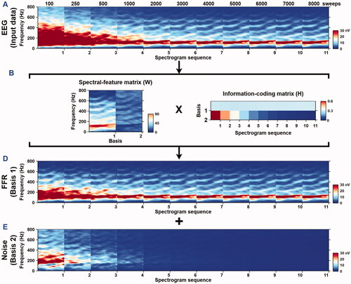
Spectral energies of the recordings obtained in adult participants were visualised in the grand-averaged spectrograms of the EEG input data (Figure 4A), spectral-basis matrix (Figure 4B), information-coding matrix (Figure 4C), enhanced FFRs (Figure 4D), and extracted noise (Figure 4E). Prior to the SSNMF decomposition, grand-averaged spectrograms showed visually discernible spectral energies following the stimulus F0 and its harmonics, starting from about 2000 sweeps (Figure 4A). After the SSNMF decomposition, grand-averaged spectrograms of the extracted FFR (Figure 4D) exhibited visually identifiable spectral energies following the stimulus F0 and its harmonics, starting from about 500 sweeps. Such an enhancement in FFR visibility was due to the fact that a substantial amount of noise (Figure 4E) was extracted through the SSNMF algorithm. The spectral-feature matrix (W in Figure 4B) optimised through the SSNMF algorithm contained two bases, where the algorithm-learned FFR and noise were clearly discernible. Similar results were observed when this algorithm was applied to individual participant (see Supplementary Figure 1, which shows the SSNMF decomposition results for recordings obtained from an adult participant).

Figure 4. Application of the SSNMF algorithm on EEG recordings obtained in adult participants. Grand-averaged spectrograms of the input data (A), spectral-basis matrix (B), information-coding matrix (C), enhanced FFR (D), and extracted noise (E).

For the neonatal participants, spectrograms of the EEG input data (Figure 5A), spectral-basis matrix (Figure 5B), information-coding matrix (Figure 5C), enhanced FFRs (Figure 5D), and extracted noise (Figure 5E) are plotted on the same graph for comparison. Spectral energies in the grand-averaged spectrograms that followed the F0 contour of the stimulus were visually discernible starting from about 1000 sweeps before the SSNMF decomposition (Figure 5A) as well as starting from about 500 sweeps after the SSNMF decomposition (Figure 5D). Such an enhancement in FFR detectability was also due to the fact that a substantiable amount of noise (Figure 5E) was removed through the SSNMF decomposition. Consistent with the FFR literature (Jeng et al. 2011; Ribas-Prats et al. 2019), response energies following the harmonics of the stimulus were clearly identifiable in adults (Figure 4) but were only faintly identifiable in neonates (Figure 5). Similar results were obtained on an individual basis (see Supplementary Figure 2, which shows the SSNMF decomposition results for recordings obtained from a neonatal participant).

Figure 5. Application of the SSNMF algorithm on EEG recordings obtained in neonatal participants. Grand-averaged spectrograms of the input data (A), spectral-basis matrix (B), information-coding matrix (C), enhanced FFR (D), and extracted noise (E).

3.2. Evaluation of the SSNMF performance

For adult participants (Figure 6), the CC values before and after the SSNMF decomposition are plotted on the same graph for comparison. Before the SSNMF decomposition (i.e. the AVG condition), the CC values (Figure 6A) were smallest at 100 sweeps and increased exponentially with increasing number of sweeps. Such increments were likely due to the effects of the conventional averaging procedure. When the SSNMF algorithm was applied (i.e. the AVG + SSNMF condition), the CC values were further increased. Such enhancements (i.e. the differences between the AVG and AVG + SSNMF conditions) were direct results of the SSNMF decomposition. The mean FFR Enhancement (Figure 6B) was 0.223, 0.159, 0.103, 0.053, 0.020, 0.012, 0.006, 0.002, 0.001, 0.000, and 0.000 at 100, 250, 500, 1000, 2000, 3000, 4000, 5000, 6000, 7000, and 8000 sweeps, respectively.

Figure 6. SSNMF performance in adult participants. A. Correlation coefficients before (i.e., the AVG condition) and after (i.e., the AVG + SSNMF condition) the SSNMF decomposition. B. FFR Enhancement as a function of the number of sweeps. C. RMSEs before (i.e., the AVG condition) and after (i.e., AVG + SSNMF condition) the SSNMF decomposition. D. Noise Reduction with increasing number of sweeps. Each shaded area represents the SSNMF performance in terms of FFR Enhancement and Noise Reduction. Δ Correlation = correlation coefficients obtained at the AVG + SSNMF condition – correlation coefficients obtained at the AVG condition. Δ RMSE = RMSE derived at the AVG + SSNMF condition – RMSE derived at the AVG condition. Each error bar indicates one standard error.

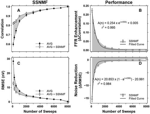
In terms of Noise Reduction, before the SSNMF decomposition (i.e. the AVG condition), the RMSE values (Figure 6C) were largest at 100 sweeps and decreased exponentially with increasing number of sweeps. Such decrements were likely caused by the effects of the conventional averaging procedure. Through the application of the SSNMF algorithm (i.e. the AVG + SSNMF condition), the RMSE values were further reduced. Such reductions (i.e. the differences between the AVG and AVG + SSNMF conditions) were direct results of the SSNMF decomposition. The mean Noise Reduction (Figure 6D) was −15.405, −8.038, −4.413, −2.199, −0.824, −0.485, −0.250, −0.089, −0.047, 0.002, and 0.351 nV at 100, 250, 500, 1000, 2000, 3000, 4000, 5000, 6000, 7000, and 8000 sweeps, respectively.

Similar results were observed for the neonatal participants (Figure 7). Specifically, the CC values (Figure 7A) increased exponentially with increasing number of sweeps prior to the SSNMF decomposition. After the SSNMF decomposition, the CC values were further increased. The mean FFR enhancement (Figure 7B) was 0.270, 0.208, 0.165, 0.106, 0.051, 0.029, 0.010, 0.005, 0.002, 0.000, and −0.001 at 100, 250, 500, 1000, 2000, 3000, 4000, 5000, 6000, 7000, and 8000 sweeps, respectively.

Figure 7. SSNMF performance in neonatal participants. A. Correlation coefficients before (i.e., the AVG condition) and after (i.e., the AVG + SSNMF condition) the SSNMF decomposition. B. FFR Enhancement as a function of the number of sweeps. C. RMSEs before (i.e., the AVG condition) and after (i.e., AVG + SSNMF condition) the SSNMF decomposition. D. Noise Reduction with increasing number of sweeps. Each shaded area represents the SSNMF performance in terms of FFR Enhancement and Noise Reduction. Δ Correlation = correlation coefficients obtained at the AVG + SSNMF condition – correlation coefficients obtained at the AVG condition. Δ RMSE = RMSE derived at the AVG + SSNMF condition – RMSE derived at the AVG condition. Each error bar represents one standard error.

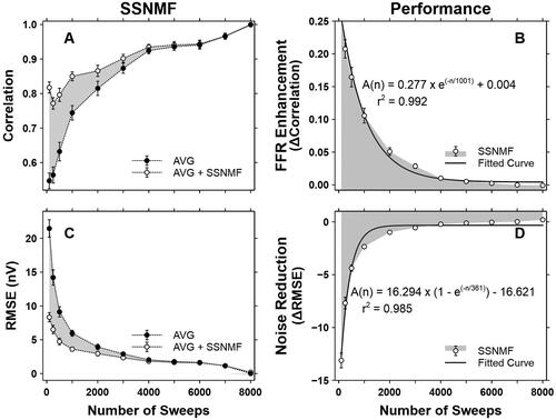
Regarding Noise Reduction, prior to the SSNMF decomposition, the RMSE values (Figure 7C) were the largest at 100 sweeps and decreased exponentially with increasing number of sweeps. After the SSNMF decomposition, the RMSE values were further reduced. The mean Noise Reduction (Figure 7D) was −13.117, −7.683, −4.384, −2.348, −0.987, −555, −0.223, −0.115, −0.045, 0.009, and 0.196 nV at 100, 250, 500, 1000, 2000, 3000, 4000, 5000, 6000, 7000, and 8000 sweeps, respectively.

3.3. Exponential modeling of the SSNMF performance

For both adult and neonatal participants, FFR Enhancement demonstrated a descending trend with an increasing number of sweeps. The resultant exponential curve-fitting models for FFR Enhancement were: (6) $$\mathit{FFR\; Enhancement\; for\; adults}=0.254\mathrm{*}\left(e^{-\frac{n}{555}}\right)+0.005$$(6) (7) $$\mathit{FFR\; Enhancement\; for\; neonates}=0.277\mathrm{*}\mathrm{ }\left(e^{-\frac{n}{1001}}\right)+0.004$$(7)

For both adult and neonatal participants, Noise Reduction exhibited an ascending trend with an increasing number of sweeps. The resultant exponential curve-fitting models were: (8) $$\mathit{Noise\; Reduction\; for\; adults}=20.653\mathrm{*}\mathrm{ }\left({1-e}^{-\frac{n}{290}}\right)-20.991$$(8) (9) $$\mathit{Noise\; Reduction\; for\; neonates}=16.294\mathrm{*}\mathrm{ }\left({1-e}^{-\frac{n}{361}}\right)-16.621$$(9)

3.4. Statistical analyses of the SSNMF performance

For FFR Enhancement, a two-way ANOVA demonstrated a significant difference for the nSweep factor (F(2.832, 79.292) = 299.440, p < 0.001, ${\eta }_p^2$ = 0.914, power = 1.000) and the age group factor (F(1, 28) = 18.168, p < 0.001, ${\eta }_p^2$ = 0.394, power = 0.984) but not the interaction between the two factors (p = 0.140). For Noise Reduction, a significant difference was observed for the nSweep factor (F(1.424, 39.864) = 359.003, p < 0.001, ${\eta }_p^2$ = 0.928, power = 1.000) but not the age group factor (p = 0.526) nor the interaction between the two factors (p = 0.140).

Two-tailed t tests demonstrated that the mean values of FFR Enhancement were statistically different (p < 0.001) from zero for all nSweep conditions except for the 6000 (p = 0.004) and 7000 (p = 0.167) sweep conditions in adult participants and the 6000 (p = 0.054) and 7000 (p = 0.823) sweep conditions in neonatal participants. The mean values of Noise Reduction were also statistically different (p < 0.001) from zero for all nSweep conditions except for the 6000 (p = 0.056) and 7000 (p = 0.858) sweep conditions in adult participants and the 6000 (p = 0.061) and 7000 (p = 0.117) sweep conditions in neonatal participants.

4. Discussion

4.1. Machine learning in improving FFR recordings

Noise is an unceasing challenge in FFR recordings. Such a challenge is particularly apparent in situations where noise is emitted from various sources with measurable amplitudes. For example, high muscle tones are often observed in participants who are unable to relax inside a sound booth. Excessive electromagnetic interference may be observed in a birth centre where many life-saving machineries must be kept running continuously. All those noises together may degrade the signal-to-noise ratio of a recording and therefore impede our ability to visualise the presence of an FFR. Many features of the FFR may be buried in the swamp of noises and thus hidden from the experimenter. In order to extract FFRs from recordings that are collected in various testing environments, finding a method (in addition to the conventional averaging procedure) that can be used to further separate the targeted FFR from noise is a much-needed request.

Although many machine learning algorithms have been employed in FFR research (Hart and Jeng 2021; Llanos, Xie, and Chandrasekaran 2017; Xie, Reetzke, and Chandrasekaran 2018; Xie, Reetzke, and Chandrasekaran 2019; Yi et al. 2017), nearly all of them are supervised machine learnings that require the experimenter to provide “gold standards” for each recording. For example, the Hidden Markov algorithm has been used to classify FFR recordings in response to four different Mandarin tones (Llanos, Xie, and Chandrasekaran 2017). With the experimenter’s knowledge and input on the correspondence between each recording and its associated Mandarin tone, the Hidden Markov algorithm is able to get 85% accuracy for Mandarin tone 2 when only 100 sweeps are included. Similarly, the gradient-boosted Decision Tree algorithm has been trained to derive 12 spectral features that are predetermined from 80 speech utterances of 40 native English speakers saying two different vowels (Yi et al. 2017). By applying the trained Decision Tree algorithm on a single-sweep basis, this algorithm can categorise FFR recordings in response to the two different English vowels by including as few as 50 sweeps. To test all algorithms that are available in the Matlab Classification Learner App, a total of 23 supervised machine learning algorithms have been evaluated (Hart and Jeng 2021). Results indicate that a majority of these algorithms are able to detect the presence or absence of an FFR in neonatal recordings with high accuracy.

It should be noted that the traditional NMF applications in audio source separation require pure signals for supervised training. The source separation algorithm used here, however, does not require the procedure of supervised training and any predetermined standards from the experimenter. Specifically, the SSNMF algorithm can learn spectral features from FFR and noise separately based on the constraint of intensities distributed across the nSweep conditions. The targeted response is then constructed by using the source-specific spectral features that are shared by all recordings. Through this process, the targeted response can be effectively enhanced, while any unrelated signals (i.e. noises) are suppressed. It is important to note that throughout this entire procedure, no subjective inputs are needed from the experimenter, which greatly facilitates the processing of FFR recordings.

4.2. Evaluation and modeling of the improvements in FFR recordings

To quantify the improvement of efficiency in FFR recordings (i.e. effectiveness of the SSNMF algorithm), exponential curve fittings are conducted on two performance indices: FFR Enhancement and Noise Reduction. Modelling results indicate that the absolute values of FFR Enhancement are the largest at 100 sweeps and decreased exponentially with increasing number of sweeps. Significant FFR Enhancement and Noise Reduction are observed when 100–5000 sweeps are included in adult and neonatal recordings. Together, these findings have confirmed the effectiveness of the SSNMF algorithm in enhancing the targeted FFRs.

For FFR Enhancement, curve fitting results have demonstrated that adult and neonatal participants have similar A_AS and A_DC values. The comparable results observed between these two groups of participants may reflect the common characteristics of the FFRs that are shared between adults and neonates. For example, some neurons in adult and neonatal auditory systems may fire action potentials with only slight or moderate neural synchrony and thus is usually undetectable in the original spectrograms when only the conventional signal averaging procedure is applied. With the proposed source separation algorithm, responses originated from those subgroups of neurons finally have a chance to be grouped together and become visually identifiable even when a low number of sweeps is included.

It is worth noting that the time constant (τ) of the fitted curve on FFR Enhancement is 555 sweeps for the adult participants and 1001 sweeps for neonates. Consistent with our previous report (Jeng et al. 2018), time constants of the fitted curves on the original portion of the FFR obtained in adults are smaller than those obtained in neonates. Such a difference may be attributed to some fundamental structural differences of the FFR between these two groups of participants who likely have distinct neural circuitries in the brainstem area. Alternatively, such a difference may also be a result of the distinct differences of the physiological and environmental noises that may be recorded in these two groups of participants (adults versus neonates) under two different testing scenarios (a sound booth in a laboratory versus a quiet room in a birth centre).

4.3. Performance of the SSNMF algorithm

Although the conventional averaging procedure may work effectively in a low-noise environment, such a procedure may be compromised when various environmental and physiological noises are embedded inside a recording. By applying the SSNMF algorithm on the EEG input data, spectral energies of the targeted FFR become visually discernible from the background noise when only 500 sweeps are included in the averaging procedure. For FFR Enhancement, the aforementioned consistent modelling outputs have demonstrated that the SSNMF algorithm performs well for recordings obtained in adult and neonatal participants.

Regarding Noise Reduction, it is worth noting that the absolute mean value of the A_DC estimates of the fitted curve for recordings obtained is 20.991 nV for the adult participants and 16.621 nV for neonates. This finding indicates that the amount of additional noise removed from adult recordings is larger than that from neonatal recordings. Such a difference may be caused by the relatively large RMSE values (mean = 28.316 nV) at 100 sweeps that is observed in adult recordings when only the conventional averaging procedure is used. In other words, the relatively larger RMSE values at 100 sweeps in adult participants (than those in the neonatal participants) may have resulted in a larger A_DC estimate on the fitted curve. Despite the relatively larger amount of noise that is present in adult recordings at 100 sweeps than those in neonatal recordings, the SSNMF algorithm works effectively for both adult and neonatal recordings.

4.4. Advantages of the SSNMF algorithm

The proposed source separation algorithm has at least two major advantages. First, the non-negative constraint ensures the assumption that brain waves are a linear sum of multiple sources. As such, the additive nature of sound amplitudes and EEG recordings are preserved. In situations where negative values exist, these values can be converted to non-negative numbers through a simple linear transformation. The second advantage is the flexible relationship between the W and H matrices. For example, when the principal component analysis (PCA) is used, orthogonality is assumed among input variables. With NMF, the W and H matrices do not have to be orthogonal, thus overcomes a traditional problem of PCA. Due to these advantages, the SSNMF algorithm was used to extract the targeted response from noise, and thus improve the efficiency of FFR recordings. Another triumph is that the SSNMF algorithm can be used in conjunction with any of the supervised machine learning algorithms that are reported in the recent FFR literature (Hart and Jeng 2021; Llanos, Xie, and Chandrasekaran 2017; Xie, Reetzke, and Chandrasekaran 2018; Xie, Reetzke, and Chandrasekaran 2019; Yi et al. 2017).

4.5. Study limitations and future directions

It is possible that the SSNMF algorithm may mistakenly consider noise as part of the targeted response (i.e. overfitting). One way to determine overfitting is to perform correlations between the extracted noise and input data that are obtained in the adult and neonatal participants (Supplementary Figure 3). Results indicate that the mean correlation coefficients are all very small, between 0.069 and 0.188 for adult participants and between 0.081and 0.280 for neonatal participants, and show no signs of increased overfitting at the high nSweep conditions. Overall, the results indicate that the SSNMF algorithm can minimise the amount of overfitting and ensure the independency of extracted FFRs and noise.

Although the SSNMF algorithm does not require any training data, performance of this algorithm relies on the quality and information that are embedded in the input spectrograms. For optimal results, this study records a maximum of 8000 sweeps from each participant. Future studies may investigate the performance of this algorithmic when only a limited number of maximal sweeps are available. Another limitation of this study is that the user must remove the silent interval to satisfy the assumption of equal response magnitudes across recording sweeps. One possible improvement is to train the spectral-basis matrix for noise (W_noise) by using only the silent interval data. The trained W_noise basis can then be used as prior knowledge to set up initial values of W_noise, so that W_noise is not initialised with random values. Such a semi-supervised learning approach may further improve the separation performance of this algorithm at a low nSweep condition. Lastly, although this study demonstrates the usefulness of the SSNMF algorithm in extracting FFRs evoked by the English vowel/i/, the applicability of this algorithm on different types of stimuli, such as the/da/stimulus that has been widely used in FFR research, remains unexplored. We encourage the user to test the performance of this algorithm by using FFRs in response to/da/and other stimuli. Despite all these limitations, the SSNMF algorithm has shown its ability to remove additional noises from the original recordings and therefore improve the efficiency of FFR recordings.

5. Conclusions

Effectiveness of the SSNMF algorithm is visualised in the sweep series of amplitude spectrograms derived from adult and neonatal recordings. The SSNMF decomposition has successfully enhanced the visibility of the FFR and removed additional noise from each recording. Such improvements are examined and modelled through exponential curve fitting of FFR Enhancement and Noise Reduction trends with increasing number of sweeps. Applications of the SSNMF algorithm on FFR recordings may prove to be useful in assessing pitch processing and neuroplasticity mechanisms in the human brain for individuals during their adulthood and immediate postnatal days.

Acknowledgments

The authors thank Dr. Amy Zidron and Dr. Brandie Nance for their assistance in recruiting neonatal participants.

Disclosure statement

No potential conflict of interest was reported by the author.

Additional information

Funding

The author(s) reported there is no funding associated with the work featured in this article.

References

- Chandrasekaran, B., J. Hornickel, E. Skoe, T. Nicol, and N. Kraus. 2009. “Context-Dependent Encoding in the Human Auditory Brainstem Relates to Hearing Speech in Noise: Implications for Developmental Dyslexia.” Neuron 64 (3): 311–319. doi:10.1016/j.neuron.2009.10.006.
- Font-Alaminos, Marta., Miriam. Cornella, Jordi. Costa-Faidella, Amaia. Hervás, Sumie. Leung, Isabel. Rueda, Carles. Escera, et al. 2020. “Increased Subcortical Neural Responses to Repeating Auditory Stimulation in Children with Autism Spectrum Disorder.” Biological Psychology 149: 107807. doi:10.1016/j.biopsycho.2019.107807.
- Hart, B., and F.-C. Jeng. 2018. “Machine Learning in Detecting Frequency-following Responses.” Proceedings of Meetings on Acoustics 35 (1): 050002.
- Hart, B. N., and F.-C. Jeng. 2021. “A Demonstration of Machine Learning in Detecting Frequency following Responses in American Neonates.” Perceptual and Motor Skills 128 (1): 48–58. doi:10.1177/0031512520960390.
- Heard, Joseph, Wei‐Chen Tung, Yu‐De Pei, Tzu‐Hao Lin, Chien‐Hsiang Lin, Tomonari Akamatsu, Colin K. C. Wen, et al. 2021. “Coastal Development Threatens Datan Area Supporting Greatest Fish Diversity at Taoyuan Algal Reef, Northwestern Taiwan.” Aquatic Conservation 31 (3): 590–604. doi:10.1002/aqc.3477.
- Hornickel, J., and N. Kraus. 2013. “Unstable Representation of Sound: A Biological Marker of Dyslexia.” The Journal of Neuroscience 33 (8): 3500–3504. doi:10.1523/JNEUROSCI.4205-12.2013.
- Jeng, Fuh-Cherng., Jiong. Hu, Brenda. Dickman, Karen. Montgomery-Reagan, Meiling. Tong, Guangqiang. Wu, Chia-Der. Lin, et al. 2011. “Cross-Linguistic Comparison of Frequency-following Responses to Voice Pitch in American and Chinese Neonates and Adults.” Ear and Hearing 32 (6): 699–707. doi:10.1097/AUD.0b013e31821cc0df.
- Jeng, F.-C., C.-D. Lin, and T.-C. Wang. 2016. “Subcortical Neural Representation to Mandarin Pitch Contours in American and Chinese Newborns.” The Journal of the Acoustical Society of America 139 (6): EL190. doi:10.1121/1.4953998.
- Jeng, F.-C., B. Nance, K. Montgomery-Reagan, and C.-D. Lin. 2018. “Exponential Modeling of Frequency-following Responses in American Neonates and Adults.” Journal of the American Academy of Audiology 29 (02): 125–134. doi:10.3766/jaaa.16135.
- Kraus, Nina., Tory. Lindley, Danielle. Colegrove, Jennifer. Krizman, Sebastian. Otto-Meyer, Elaine C. Thompson, Travis. White-Schwoch, et al. 2017. “The Neural Legacy of a Single Concussion.” Neuroscience Letters 646: 21–23. doi:10.1016/j.neulet.2017.03.008.
- Kraus, Nina., Elaine C. Thompson, Jennifer. Krizman, Katherine. Cook, Travis. White-Schwoch, and Cynthia R. LaBella. 2016. “Auditory Biological Marker of Concussion in Children.” Scientific Reports 6: 39009. doi:10.1038/srep39009
- Krishnan, A., Y. Xu, J. T. Gandour, and P. A. Cariani. 2004. “Human Frequency-following Response: Representation of Pitch Contours in Chinese Tones.” Hearing Research 189 (1–2): 1–12. doi:10.1016/S0378-5955(03)00402-7.
- Lee, D. D., and H. S. Seung. 1999. “Learning the Parts of Objects by Non-Negative Matrix Factorization.” Nature 401 (6755): 788–791. doi:10.1038/44565
- Li, X., and F.-C. Jeng. 2011. “Noise Tolerance in Human Frequency-following Responses to Voice Pitch.” The Journal of the Acoustical Society of America 129 (1): EL21–EL26. doi:10.1121/1.3528775.
- Lin, T.-H., T. Akamatsu, F. Sinniger, and S. Harii. 2021a. “Exploring Coral Reef Biodiversity via Underwater Soundscapes.” Biological Conservation. 253: 108901. doi:10.1016/j.biocon.2020.108901.
- Lin, T.-H., T. Akamatsu, and Y. Tsao. 2021b. “Sensing Ecosystem Dynamics via Audio Source Separation: A Case Study of Marine Soundscapes off Northeastern Taiwan.” PLoS Computational Biology 17 (2): e1008698. doi:10.1371/journal.pcbi.1008698.
- Lin, T.-H., S.-H. Fang, and Y. Tsao. 2017. “Improving Biodiversity Assessment via Unsupervised Separation of Biological Sounds from Long-Duration Recordings.” Scientific Reports 7 (1): 4547. doi:10.1038/s41598-017-04790-7
- Lin, T.-H., and Y. Tsao. 2020. “Source Separation in Ecoacoustics: A Roadmap towards Versatile Soundscape Information Retrieval.” Remote Sensing in Ecology and Conservation 6 (3): 236–247. doi:10.1002/rse2.141.
- Llanos, F., Z. Xie, and B. Chandrasekaran. 2017. “Hidden Markov Modeling of Frequency-following Responses to Mandarin Lexical Tones.” Journal of Neuroscience Methods 291: 101–112. doi:10.1016/j.jneumeth.2017.08.010.
- Musacchia, Gabriella., Jiong. Hu, Vinod K. Bhutani, Ronald J. Wong, Mei-Ling. Tong, Shuping. Han, Nikolas H. Blevins, et al. 2020. “Frequency-following Response among Neonates with Progressive Moderate Hyperbilirubinemia.” Journal of Perinatology 40 (2): 203–211. doi:10.1038/s41372-019-0421-y.
- Rauterkus, G., D. Moncrieff, G. Stewart, and E. Skoe. 2021. “Baseline, Retest, and Post-Injury Profiles of Auditory Neural Function in Collegiate Football Players.” International Journal of Audiology 60 (9): 650–662. doi:10.1080/14992027.2020.1860261.
- Ribas-Prats, Teresa., Laura. Almeida, Jordi. Costa-Faidella, Montse. Plana, M. J. Corral, M. Dolores. Gómez-Roig, Carles. Escera, et al. 2019. “The Frequency-following Response (FFR) to Speech Stimuli: A normative dataset in healthy newborns.” Hearing Research 371: 28–39. doi:10.1016/j.heares.2018.11.001.
- Russo, N. M., E. Skoe, B. Trommer, T. Nicol, S. Zecker, A. Bradlow, N. Kraus, et al. 2008. “Deficient Brainstem Encoding of Pitch in Children with Autism Spectrum Disorders.” Clinical Neurophysiology 119 (8): 1720–1731. doi:10.1016/j.clinph.2008.01.108.
- Skoe, E., and N. Kraus. 2010. “Auditory Brain Stem Response to Complex Sounds: A Tutorial.” Ear and Hearing 31 (3): 302–324. doi:10.1097/AUD.0b013e3181cdb272.
- Smaragdis, P., C. Févotte, G. J. Mysore, N. Mohammadiha, and M. Hoffman. 2014. “Static and Dynamic Source Separation Using Nonnegative Factorizations: A Unified View.” IEEE Signal Processing Magazine 31 (3): 66–75. doi:10.1109/MSP.2013.2297715.
- Van Dyke, K. B., R. Lieberman, A. Presacco, and S. Anderson. 2017. “Development of Phase Locking and Frequency Representation in the Infant Frequency-following Response.” Journal of Speech, Language, and Hearing Research 60 (9): 2740–2751. doi:10.1044/2017_JSLHR-H-16-0263.
- Xie, Z., R. Reetzke, and B. Chandrasekaran. 2019. “Machine Learning Approaches to Analyze Speech-Evoked Neurophysiological Responses.” Journal of Speech, Language, and Hearing Research 62 (3): 587–601. doi:10.1044/2018_JSLHR-S-ASTM-18-0244.
- Xie, Z., R. Reetzke, and B. Chandrasekaran. 2018. “Taking Attention Away from the Auditory Modality: Context-Dependent Effects on Early Sensory Encoding of Speech.” Neuroscience 384: 64–75. doi:10.1016/j.neuroscience.2018.05.023.
- Yi, H. G., Z. Xie, R. Reetzke, A. G. Dimakis, and B. Chandrasekaran. 2017. “Vowel Decoding from Single-Trial Speech-Evoked Electrophysiological Responses: A Feature-Based Machine Learning Approach.” Brain and Behavior 7 (6): e00665. doi:10.1002/brb3.665.