Optimised adaptive procedures and analysis methods for conducting speech-in-noise tests

Abstract

Objective

Speech-in-noise testing is a valuable part of audiological test batteries. Test standardisation using precise methods is desirable for ease of administration. This study investigated the accuracy and reliability of different Bayesian and non-Bayesian adaptive procedures and analysis methods for conducting speech-in-noise testing.

Design

Matrix sentence tests using different numbers of sentences (10, 20, 30 and 50) and target intelligibilities (50 and 75%) were simulated for modelled listeners with various characteristics. The accuracy and reliability of seven different measurement procedures and three different data analysis methods were assessed.

Results

The estimation of 50% intelligibility was accurate and showed excellent reliability across the majority of methods tested, even with relatively few stimuli. Estimating 75% intelligibility resulted in decreased accuracy. For this target, more stimuli were required for sufficient accuracy and selected Bayesian procedures surpassed the performance of others. Some Bayesian procedures were also superior in the estimation of psychometric function width.

Conclusions

A single standardised procedure could improve the consistency of the matrix sentence test across a range of target intelligibilities. Candidate adaptive procedures and analysis methods are discussed. These could also be applicable for other speech materials. Further testing with human participants is required.

Keywords:

• Adult or general hearing screening
• speech intelligibility
• speech-in-noise
• psychoacoustics/hearing science

1. Introduction

Speech-in-noise (SIN) testing yields important information beyond audiometric thresholds, can be used to assess the benefit of hearing interventions, and is thus a valuable part of audiological test batteries. However, despite a call for clinical audiologists to use outcome measures that determine the efficacy of interventions, SIN testing is often not performed in audiological practice (Duncan and Aarts 2006). Therefore it is important that SIN testing can be carried out efficiently and in a standardised manner, such that it is straightforward and quick for clinicians to administer.

SIN performance, i.e. probability of correct word recognition as a function of the signal-to-noise ratio (SNR), can be described by a psychometric function (PF) (Hu, Swanson, and Heller 2015). The PF can be characterised by its slope, the rate at which performance changes as a function of SNR, and its inflection point, the mid-point between chance level and 100% performance. Two other “nuisance” parameters (Prins 2013) can be added to obtain more complex PF models; guessing (the probability of a correct response at inaudible levels) and lapsing (the probability of an incorrect response at clearly audible levels). Often SIN testing is performed to derive the threshold; the SNR required to reach a given level of performance. This is referred to as the Speech Reception Threshold (SRT), with the level of performance normally being defined as 50% (i.e. SRT₅₀).

The underlying PF of an individual listener can be inferred from a pattern of responses across a range of SNRs. The selection of these SNRs can be fixed, using a constant number of measurements. This is known as the “Method of Constant Stimuli” (Leek 2001), an approach which can be prone to floor or ceiling effects (Nilsson, Soli, and Sullivan 1994), given that the fixed range of SNRs could be remote from the true threshold and thus provide little information (Watson and Fitzhugh 1990). Furthermore, this approach requires a large number of trials and is thus time consuming (Leek 2001; Watson and Fitzhugh 1990).

Adaptive stimulus placement procedures can facilitate more efficient measurements of the PF (e.g. Kontsevich and Tyler 1999). They can be used to approximate the entire PF (e.g. Shen and Richards 2012), but can also be concentrated on efficiently measuring specific PF parameters. For example, in order to estimate a given SRT, stimuli are most optimally placed at the intensity corresponding to the targeted performance level (Prins 2013). This is a commonplace practice for SIN testing, with the SRT for 50% intelligibility (SRT₅₀) often being sought (e.g. Brand and Kollmeier 2002). However, Naylor (2016) argues that there are potential drawbacks of using adaptive techniques targeting SRT₅₀. A principal issue is that such tests might result in SNRs which are not ecologically valid (Smeds, Wolters, and Rung 2015; Wu et al. 2018). Indeed, Brand and Kollmeier (2002) suggest that intelligibilities of beyond about 80% hold most audiological relevance. A higher point of intelligibility on the PF would thus have to be targeted (Keidser et al. 2013).

A further advantage of adaptive procedures is that they can mitigate floor and ceiling effects, given that stimulus levels are selected based on an individual listener’s responses. Furthermore, some of these procedures place stimuli to optimise information gain about a listener’s PF. Therefore, the number of trials required to reach a given estimation accuracy could be reduced. This makes them well suited for clinical application.

The adaptive procedure of Brand and Kollmeier (2002) has been optimised for use with a common clinical and research tool; the matrix sentence test (Wagener, Brand, and Kollmeier 1999a, 1999b; Wagener, Kühnel, and Kollmeier 1999). Using this adaptive procedure with the supplied test material is reported to provide efficient, reliable and comparable speech reception thresholds across different languages (Kollmeier et al. 2015). However, the procedure selects stimuli assuming a fixed PF slope value (0.15 dB⁻¹), independent of prior listener responses and the level of intelligibility that is being tracked. This may be problematic because steps sizes could be suboptimal for higher target percent correct levels (PC) (where the PF slope is shallower) and listeners with differing PF slopes, potentially leading to inefficient stimulus placement. Furthermore, this procedure reduces its stimulus step size as a function of the number of stimulus reversals, regardless of the reliability of listener responses. This might lead to a situation in which stimuli are placed remotely from the true threshold, with the adaptive procedure being incapable of efficiently moving back towards the true threshold.

The procedure by Brand and Kollmeier (2002) might be improved upon by implementing work investigating the use of Bayesian adaptive procedures. These procedures perform running estimations of the listener’s PF, given previous trial data, and subsequently place stimuli to maximise information gain or minimise expected entropy, variance, or uncertainty in parameter estimates (Doire, Brookes, and Naylor 2017; Remus and Collins 2008; Shen and Richards 2012; Shen, Dai, and Richards, 2015). The respective stimulus placement schemes can be selected such to target optimal sampling points associated with specific PF parameters. For example, if threshold is the parameter of interest, efficiency can be improved by accurately placing trials at threshold (Green 1990), and thus the large number of trials required for slope estimation (Macmillan and Creelman 2004; Remus and Collins 2007) can be significantly reduced.

SIN tests conducted using these procedures should, therefore, be able to derive the SRT more efficiently, i.e. fewer trials would be required for a stable and accurate estimate of SRT. Beyond this, the procedures should also offer increased accuracy for measurements of different target PCs, since they do not assume a fixed slope. Thus, while the procedure of Brand and Kollmeier (2002) is optimised to estimate SRT₅₀, Bayesian procedures should also give reasonable results for other speech intelligibility levels, while potentially providing a more efficient approach.

Apart from the placement of stimuli during measurements, another important consideration is how subsequent data analysis should be carried out on listener responses. For adaptive procedures tracking a single point on the PF, one approach could be to take an average of stimulus presentation levels over trials fulfilling a certain criterion (e.g. the stimuli SNRs over the last 10 trials)—this is often the approach taken in a clinical setting (HörTech gGmbH Oldenburg 2011). Another approach would be to fit a PF to response data and derive the resulting SRT. Such an approach can be optimised by concentrating observations at given points on the PF, depending on the parameter of interest (Prins 2013). Nevertheless, a suboptimal dataset, which has not correctly tracked optimal probe SNRs, could limit the accuracy with which the PF will be fitted. Furthermore, erratic responses given by the listener could also serve to limit the accuracy of fitted PFs. One method, which employs Bayesian estimation of PFs, allows for overdispersion in observations (Schütt, Harmeling, Macke, and Wichmann 2016), and could therefore be advantageous in situations with unreliable listeners. This method also models guessing and lapsing rates, which could serve to reduce estimation errors for threshold and slope parameters (Prins 2013).

The aim of this study is to investigate whether the use of adaptive Bayesian testing procedures and analysis methods derive more accurate, more reliable, and more efficient estimates of SRTs than a currently implemented clinical approach (Brand and Kollmeier 2002). The goal was to identify standardised methods which could be used to improve and expedite the administration of clinical and research SRT test procedures. For this reason the investigation is centred on a commonly-used SIN test in German-speaking countries; the matrix sentence test (MST) (Wagener, Brand, and Kollmeier 1999a, 1999b; Wagener, Kühnel, and Kollmeier 1999), though it is feasible that the procedures investigated would be applicable for other speech test material. Data simulations, which are a common approach in the investigation of psychometric procedures (e.g. Remus and Collins 2008; Fründ, Haenel and Wichmann 2011; Shen and Richards 2012; Doire, Brookes, and Naylor 2017), were used to investigate the efficacy of different approaches to the measurement and analysis of the MST.

2. Materials & methods

2.1. Listener characteristics

1000 listeners were simulated with an underlying “true” PF ($\psi$). $\psi$ for a given SNR ($x$) was defined as a transformed logistic function, with threshold, slope, guessing rate, and lapsing rate parameters denoted as α, β, γ, and λ, respectively: (1) $$\psi \left(x;\alpha ,\beta ,\gamma ,\lambda \right)=\gamma +\frac{1-\gamma -\lambda }{{1+e}^{-\beta (x-\alpha )}}$$(1)

For each simulated listener, $\alpha$ and $\beta$ were drawn from a uniform distribution: $\alpha \sim U(-10\mathrm{ }dB,20\mathrm{ }dB)$ and $\beta \sim U({0.2\mathrm{ }dB}^{-1},{1\mathrm{ }dB}^{-1}).$ The range for $\beta$ was selected based on previous research (Kollmeier and Wesselkamp 1997; Wagener, Brand, and Kollmeier 1999a, 1999b; Wagener, Kühnel, and Kollmeier 1999), given that the MST speech material results in specifically steep PFs (Brand and Kollmeier 2002). The range for $\alpha$ was selected to give an assortment of different SRTs, based on previously reported reference data across different degrees of hearing loss from the MST (Kollmeier et al. 2015; Wardenga et al. 2015).

In this study we modelled the “open” version of the MST, during which listeners are asked to simply repeat back what they have heard. Given there are a finite number of responses to the MST (10 for each of the 5 word positions), it is feasible that listeners could correctly guess words. However, it was also presumed that listeners have different capacities for correctly remembering all possible words. A guessing rate was therefore drawn from another uniform distribution $\gamma \sim U(0\mathrm{\%},10\mathrm{\%}).$ Similarly, lapsing was modelled by randomly drawing from a uniform distribution: $\lambda \sim U(0\mathrm{\%},20\mathrm{\%}).$ This range could be considered to extend to a relatively high lapsing rate compared with other research (Doire, Brookes, and Naylor 2017), but was chosen to allow investigating the effects of highly unreliable listeners.

2.2. Response modelling

For individual simulated listeners, responses could have simply been drawn from a binomial distribution with the response probability ${\psi }_x$ from the respective listener’s PF. However, fluctuations in attention or motivation and learning lead to noisy responses and might make some portions of the test less reliable than others. Therefore, we modelled this aspect probabilistically as described by Fründ, Haenel, and Wichmann (2011). For each trial, the correct response probability at a given input SNR was itself a beta-distributed random variable with mean ${\psi }_x.$ Thus, the Beta distribution’s parameters $q$ and $t$ were chosen according to Equation (2)(2) $${\psi }_x=\frac{t}{t+q}$$(2) . Note that the mean of the beta distribution was used (Schütt et al. 2016), as opposed to the mode (Fründ et al. 2011), in order to avoid biasing responses. (2) $${\psi }_x=\frac{t}{t+q}$$(2)

The sum of these two parameters ($M=t+q$) determined the width of the beta distribution. As in Fründ, Haenel, and Wichmann (2011), the value of $M$ was fixed at 10 in this study in order to model participant fluctuation and add a layer of realism to simulations. Given that the performance of practice lists should minimise learning effects on the MST (Kollmeier et al. 2015), this aspect of performance fluctuation was not modelled.

2.3. Adaptive test procedures

With the simulated listeners, seven different adaptive procedures were used to generate speech test data based on the MST.

The first was a reference condition (Reference); the commonly used adaptive procedure reported by Brand and Kollmeier (2002). This procedure selected the next stimulus SNR based on the listener’s response to the previous sentence only, and how many stimulus reversals there had been according to Equation (3)(3) $$\Delta \mathit{SNR}=-\frac{f\left(i\right)\cdot (\mathit{prev}-\mathit{tar})}{\mathit{slope}}$$(3) . (3) $$\Delta \mathit{SNR}=-\frac{f\left(i\right)\cdot (\mathit{prev}-\mathit{tar})}{\mathit{slope}}$$(3)

Here tar was the target PC, prev was the percent words correct from the previous sentence, slope was the slope of the PF at the specified target PC, i was the number of reversals of presentation level, and f was a parameter that controlled the rate of convergence. f was calculated as: $f(i)=1.5\cdot {1.14}^{-i},$ with its final value limited to 0.1, and the slope parameter was fixed at 0.15 dB⁻¹ (Brand and Kollmeier 2002). The second procedure (modReference) was identical to Reference, but limited the final value of $f(i)$ to 0.25 and used a fixed slope parameter of 0.1 dB⁻¹. This approach assumed a flatter PF slope, allowed for larger step sizes than the original procedure of Brand and Kollmeier (2002), and corresponded to the current software implementation (HörTech gGmbH Oldenburg 2019) of the Reference adaptive procedure (Wagener 2021).

The third procedure (Interleaved) followed the same approach as Reference but used two randomly interleaved adaptive tracks targeting two different fixed levels of intelligibility; 20% and 80% respectively. Brand and Kollmeier (2002) specify that this approach should be used with a minimum of 30 sentences if the measurement of slope is sought. The approach here was not to measure slope per se, rather different target PCs, but this procedure was included as it was thought accurate slope estimation might be important for establishing different SRTs.

The remaining stimulus placement methods were adaptive parametric procedures, which placed stimuli based on all previous responses (Remus and Collins 2008; Doire et al. 2017; Shen, Dai, and Richards 2015). These methods assumed a form of the PF (in this study a logistic function) and continually provided an estimate of the PF parameters. The way stimulus placement proceeded, however, differed between the different procedures.

Two of these procedures were based on work published by Remus and Collins (2008), which describes different stimulus placement strategies maximising information gain for various aspects of the PF. Therefore, in principle, using these methods allowed for the targeting of specific information from the PF with maximal efficiency. The first of these strategies, Fisher Information Gain (FIG), calculated the expected increase in Fisher information (Cover and Thomas 2006; Remus and Collins 2008) for each possible specified stimulus value and then selected the next level to maximise the information gain. In this FIG procedure, the Fisher information metric considered both PF threshold and slope parameters. Thus, stimuli were selected that simultaneously maximised information gain for threshold and slope. The second strategy, Greedy, placed the next trial at the stimulus value closest to the running estimate of the threshold. This procedure ignored the slope parameter and selected stimuli that maximised information gain for PF threshold alone. The PF model used by Remus and Collins (2008, see their Equation 1) included guessing and lapsing rate parameters, here denoted as γ and λ, respectively. We introduced an additional parameter ζ, which allowed the specification of the target PC for measurement. The updated definition was: (4) $$p(x;\alpha ,\beta ,\gamma ,\lambda ,\zeta )=\min \left[\gamma +\frac{1-\gamma }{1+e^{-\beta \left(x-\alpha \right)+\zeta }},\mathrm{ }1-\lambda \right]$$(4)

Given a correct-response target probability of P_t at threshold (on the PF unscaled by the guessing rate γ), the value of ζ was chosen as $\ln \mathrm{(}\frac{1}{P_t}-\mathrm{1)}$.

A further Bayesian procedure described by Doire et al. (2017) was also included in the study (Adaptive grid). This approach differed in that it used an adaptive grid for the PF parameters, meaning that a range of possible PF parameters did not need to be specified in advance (as was the case for the other three Bayesian procedures). Similarly to the above FIG procedure, the Adaptive Grid procedure optimised the measurement of both threshold and slope simultaneously. It was implemented using the “v_psycest” function from the Voicebox Toolbox for Matlab (Brookes 2021).

A final procedure, UML (Shen and Richards 2012; Shen, Dai, and Richards, 2015), was also investigated. Unlike the above methods, this Bayesian procedure treated the lapsing rate as a free parameter which was estimated. To this end, the procedure continually updated its estimates of PF parameters and identified four measurement “sweet points” associated with minimising the expected variance in the estimation of different parameters of the PF; threshold, lapsing and two different locations for slope. It then adaptively cycled through these sweet points using an n-down, 1-up rule (in this study a 2-down, 1-up rule was selected as per the recommendation of Shen, Dai, and Richards, 2015). The procedure thus sampled from the entire PF, rather than focussing specifically on a single point¹. Given its ability to freely estimate lapsing rate, this procedure could be particularly useful in cases where the lapsing rate of listeners is high and may bias PF estimates (Prins 2013). For this reason it was included in this study and was implemented using version 2.2 of the “UML” toolbox for Matlab described by Shen, Dai, and Richards (2015).

To summarise, a total of seven adaptive stimulus placement procedures were investigated. These are summarised in Table 1, alongside specific information for each procedure. For the Bayesian placement procedures, a parameter space (a grid of potential PF parameters), a stimulus space (a grid of potential test SNRs) and a prior had to be specified. Note that all procedures were started at an SNR of 20 dB in order to be consistent and provide the first stimulus at a clearly audible level for listeners. This is an explicit recommendation for several of the procedures tested (Remus and Collins 2008; Shen and Richards 2012; Shen, Dai, and Richards, 2015).

Table 1. Adaptive stimulus placement procedures investigated in this study. The prior and parameter and stimulus spaces are specified for each respective method.

Procedure	Prior	Parameter space	Stimulus space
Reference	N/A	N/A	[−20,20]
modReference	N/A	N/A	[−20,20]
Interleaved	N/A	N/A	[−20,20]
FIG	Flat	α = linspace^a(−10,20,81)	linspace(−20,20,81)
		Width^b = linspace(2,30,11)
		γ = 0.02
		λ = 0.02
Greedy	Flat	α = linspace(−10,20,81)	linspace(−20,20,81)
		Width = linspace(2,30,11)
		γ = 0.02
		λ = 0.02
Adaptive Grid	Gaussian	Starting values for the adaptive grid:	linspace(−20,20,81)
		α = linspace(−20,20,81)
		β = linspace(0.2,2,11)
		γ = 0.02
		λ = 0.02
UML	Flat	α = linspace(−20,20,81)	[−20,20]
		β = logspace^c(0.2,2,11)
		γ = 0.02
		λ = linspace(0,0.2,5)

^a linspace(x₁, x₂, n) represents n linearly spaced values between x₁ and x₂.

^b The width of the PF was defined as the difference in SNR between the 5% and 95% correct intelligibility points on the unscaled PF (i.e. before the guessing and lapsing parameters are applied).

^c logspace(x₁, x₂, n) represents n logarithmically spaced values between x₁ and x₂.

Also note that, in accordance with the MST, each stimulus consisted of a sentence of five words presented at a given SNR. The test was scored on a words-correct basis, and a new stimulus level was selected for each new sentence. For the Bayesian methods used in this study, the posterior was updated following each word, and the next stimulus SNR was selected from the suggestion given following the last word of the sentence.

2.4. Procedure

For each of the 1000 simulated listeners, test simulations were run at each of two target PCs (50% and 75%) and for each of four list lengths (10, 20, 30 and 50 sentences). Each combination of these setups and adaptive procedures was run three times (to provide three test-retest occasions for each condition) with listener responses being generated according to the aforementioned model. This resulted in a total of 168 speech tests for each simulated listener; 7 (procedures) by 2 (target PCs) by 4 (list lengths) by 3 (retest occasions).

Although 50% intelligibility is commonly used as a target PC, 75% was also included in this study, as it is becoming increasingly important to test at more favourable SNRs to retain ecological validity (Keidser et al. 2013; Naylor, 2016). The selection of 75% intelligibility here was based on previous work (Doire et al, 2017) and the sentiment that higher intelligibility levels hold greater ecological relevance (Brand and Kollmeier, 2002). List lengths of 20 and 30 sentences were chosen given previous findings of Brand and Kollmeier (2002). 10 sentence lists were included to investigate whether measurement efficiency could be improved with fewer trials, without compromising accuracy or reliability. In addition, 50 sentence lists were included to investigate whether more trials would maximise accuracy and reliability at the cost of efficiency.

2.5. SRT calculation methods

Data resulting from the simulated listeners for each of the aforementioned adaptive procedures were subjected to two different SRT calculation methods. The first (referred to here as Posterior) derived the SRT from the posteriors given by the parametric procedures². As suggested by Shen, Dai, and Richards (2015), the mean of the posterior distribution was used to estimate PF parameters at the end of each test. These parameters were then used to calculate the specified SRT and PF width, based on the definition of the PF given for each respective procedure.

The second analysis method (named here Beta) extended the binomial model, often used for PF fitting, to a beta-binomial model, which accounted for sources of overdispersion in the data (described in detail by Schütt et al. 2016). In addition to SRT and PF width, this approach allowed for the estimation of guessing and lapsing rates, which can influence SRT and slope estimates (Prins, 2013). This method was implemented using the Psignifit 4 toolbox for Matlab (Schütt et al. 2016). A logistic sigmoid was employed, and per Schütt et al.’s (2016) recommendation for the Psignifit 4 method, the maximum of the posterior distribution was used to estimate the PF parameter. The number of parameter grid points were as follows: 40 for threshold and slope, 20 for guessing and lapsing rates and 20 for variance scaling. Stimulus pooling was undertaken for trials where presentation SNRs lay within 0.4 dB of each other. In practical terms this meant that pooling was undertaken for the reference procedures (Reference, modReference and interleaved), but none of the Bayesian procedures (where the SNR resolution was 0.5 dB).

An additional analysis method (henceforth referred to as Averaging) was also applied for the Reference and modReference adaptive procedures. In this case the SRT was calculated as the mean presentation SNR from sentence 12 to the end of the test, including the next projected test SNR (i.e. for a 20-sentence list, sentences 12–21 and for a 30-sentence list, sentences 12–31). This is the scoring technique given in the user manual of the German version of the MST (Oldenbuger Satztest; OLSA) (HörTech gGmbH Oldenburg, 2011). Given that this calculation was not possible for 10 sentence lists, for this number of trials an average was only taken for the final 5 stimulus sentences, including the next projected test SRT (i.e. sentences 7–11).

2.6. Analysis

The PF width and SRT estimates for each procedure and analysis method were assessed in terms of their bias, their absolute error, and their test-retest reliability over the three repeated test occasions (i.e. whether they resulted in stable estimates at different test occasions). These attributes were also investigated independently for the procedure and analysis method combinations during different test setups (i.e. 10 vs 20 vs 30 vs 50 sentences, or with a target PC of 50% vs 75%). The “true” SRT of listeners was defined as the SNR required for the target PC on the PF scaled by the listener’s guessing and lapsing rates. The PF width was analysed instead of PF slope, to allow for a comparison across all procedures. This width was defined as the difference in SNR between the 5% and 95% correct intelligibility points on the unscaled PF (i.e. before the guessing and lapsing parameters were applied) (cf. Schütt et al. 2016).

To investigate test-retest reliability, the intraclass correlation coefficient (ICC) was calculated for each simulated listener and test condition across the three test occasions. ICCs reflect the degree of correlation and agreement between three or more measurements and consist of a value in the range 0 to 1 (Koo and Li 2016). As a rule of thumb, values of <0.5 reflect poor reliability, 0.5–0.75 reflect moderate reliability, 0.75–0.9 reflect good reliability, and >0.9 reflect excellent reliability. A two-way effects, absolute agreement, single rater/measurement model (Koo and Li 2016) was fitted using the irr package (v0.84.1; Gamer et al. 2019) for R (v4.0.3; R Core Team 2013).

3. Results

Figure 1 shows the results for a target of SRT₅₀ by plotting the accuracy and reliability of threshold estimates together, as well as visualising the bias associated with each adaptive procedure and analysis method combination. In the lower panels, ICCs are depicted on the x-axis and absolute errors on the y-axis. Thus, better procedures are located towards the bottom right of the plots (high ICCs and small errors), while poorer procedures are located towards the top left (low ICCs and larger errors). Respective biases of each procedure and analysis combination are then shown in the upper panels.

Figure 1. Accuracy (absolute error in dB), bias (dB) and reliability (ICC) of each analysis-procedure combination for a target of SRT₅₀. Error bars indicate 95% confidence interval of the means.

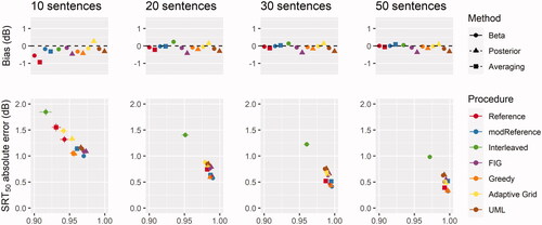
In general, it appeared possible to measure SRT₅₀ repeatably, with little bias and a high degree of accuracy (to within 0.5 dB on average with the most accurate test setups and sufficient trials). Notably this was the case for the standard clinical procedure currently implemented in the official MST software, which showed minimal bias and was amongst the most accurate and reliable procedures. Estimates of SRT₅₀ with an absolute error of around 1 dB also seemed feasible with as few as 10 sentences, depending on the procedure and analysis combinations being used. Specifically, the use of Beta as an analysis method compared to Averaging appeared to facilitate the estimation of SRT₅₀ when there were very few trials. Generally, SRT₅₀ was most accurately and repeatably estimated using procedures which aimed to place stimuli as close as possible to threshold (i.e. Greedy, Reference & modReference). However, other methods which additionally prioritised the measurement of slope (e.g. AdaptiveGrid, FIG & UML) did not compromise repeatability or accuracy of SRT₅₀ estimates.

Figure 2 visualises data in the same manner as above, but for a target of SRT₇₅. There was a notable decrease in accuracy when measuring SRT₇₅; the most accurate procedure/analysis combinations only estimated SRT₇₅ to within an error of 1 dB (even with 50 sentences), although reliability remained excellent. Provided that this is an acceptable degree of error, the simulations suggest that measurements targeting SRTs of higher than 50% are possible, though more sentences may be necessary. Here the opposite trend was observed compared to the estimation of SRT₅₀; procedures which attempted to characterise slope accurately (e.g. AdaptiveGrid, FIG & UML) performed better than the Reference and modReference procedures that focussed only on SRT. The Greedy procedure was an exception to this rule, also estimating SRT₇₅ with a good degree of accuracy and reliability. This procedure attempted to place stimuli at the 75% correct level of the unscaled PF (see Equation 4(4) $$p(x;\alpha ,\beta ,\gamma ,\lambda ,\zeta )=\min \left[\gamma +\frac{1-\gamma }{1+e^{-\beta \left(x-\alpha \right)+\zeta }},\mathrm{ }1-\lambda \right]$$(4) ).

Figure 2. Accuracy (absolute error in dB), bias (dB) and reliability (ICC) of each analysis-procedure combination for a target of SRT₇₅. Error bars indicate 95% confidence interval of the means.

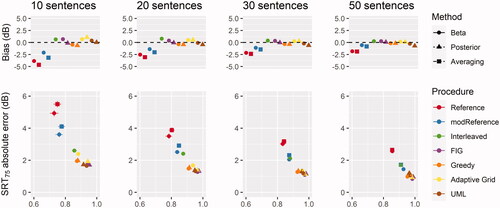
The poor performance of the reference procedures here appeared to result from a negative bias in SRT estimation. That is to say that SRTs were consistently estimated as more positive than the true value. This appeared to be related to stimulus placements, rather than the analysis carried out, because the SRT estimation method Beta also showed a repeatable negative bias (besides for 50 sentence trials). To investigate where each procedure placed stimuli during measurements, stimulus placements were visualised as a function of their corresponding speech intelligibility on the true PF for each individual listener (see Figure 3).

Figure 3. Histograms of stimulus placements corresponding to individual listener’s intelligibilities with target intelligibilities of 50% (top row) and 75% (bottom row) respectively.

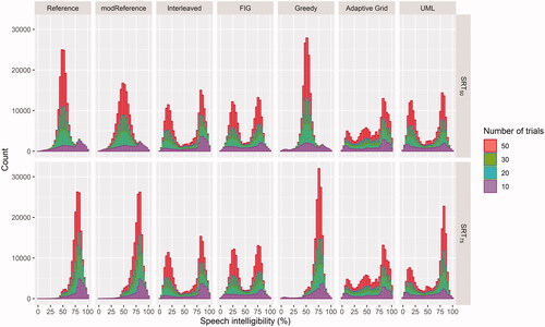
It is clear that some procedures targeting the measurement of the entire PF (Adaptive Grid, FIG, Interleaved & UML) retained similar stimulus placement strategies, independent of the targeted SRT. This is in contrast to procedures which specifically targeted a given SRT (Greedy, Reference & modReference). These placement procedures clearly changed strategy depending on the SRT specified. When targeting SRT₇₅, Reference and modReference seemed to place more stimuli than Greedy at very high regions of the PF. Across all trials aimed at estimating SRT₇₅, Reference, modReference and Greedy placed 28%, 24% and 10% of their trials respectively at intelligibilites of greater than 85%.

The majority of procedures aimed at measuring the entire PF generally placed stimuli at two distinct regions either side of threshold, though FIG appeared to be more consistent than UML and Interleaved in placing trials to similar extents below and above threshold. Specifically, the stimulus placement of Interleaved did not appear accurate at all in its targeting of 80% intelligibility. One method which appeared different to the others was Adaptive Grid, which focused many of its stimulus placements at SRT₅₀, but also spread presentations at other areas of the PF. This pattern became more marked as the number of sentences increased. In fact, for all placement procedures, the more presentations there were, the clearer the stimulus placement strategy became.

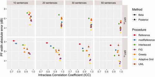
Figure 4 shows the reliability and absolute error associated with the different procedure/method combinations for PF width estimation. An increased accuracy with increasing numbers of sentences was observed. The estimates were very repeatable and most accurate for procedures which did not target SRT alone. There was a clear decrease in accuracy and reliability for such procedures (Greedy, Reference & modReference), when SRT₇₅ was targeted, as opposed to SRT₅₀.

Figure 4. Accuracy (absolute error) and reliability (ICC) of each analysis-procedure combination for PF width estimation. Error bars indicate 95% confidence interval of the means.

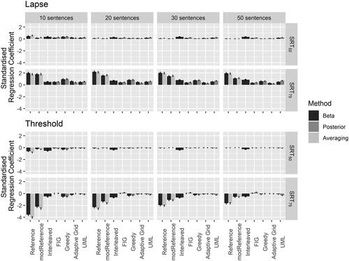
In order to investigate the dependency of SRT estimation accuracy as a function of the simulated listener characteristics, regression analyses were performed. The effect of each listener characteristic on the absolute error was estimated for every combination of procedure and method. Regression coefficients were standardised to enable direct comparisons of the effect of listener characteristics on SRT estimation accuracy between procedures and methods.

Figure 5 shows the relative importance of the threshold and lapsing rate predictors on absolute error in terms of dB change in absolute error per unit change in each standardised predictor. All procedures and methods appeared invariant to changes in guessing rate and slope (all standardised regression coefficients < 1). Therefore they are not depicted in Figure 5 to improve readability for the characteristics which did impact the accuracy of different methods and procedures³. The SRT₇₅ estimation accuracy of the reference procedures was disproportionately affected by lapsing rate and the threshold value, compared to the other stimulus placement strategies. This effect became more apparent with decreasing numbers of sentences. The influence of threshold value likely reflected slower convergence of the reference procedures to placing trials at informative levels, given a positive starting SNR. Listener lapsing could have affected the accuracy of certain procedures and methods by driving stimulus placement away from SNRs of interest. Whilst both reference procedures were affected, the greater stimulus step sizes allowed by modReference appear to have somewhat alleviated this issue. The Bayesian procedures, on the other hand, were less influenced by lapsing rate, as well as threshold values.

Figure 5. Standardised regression coefficients for lapsing rate and threshold, target intelligibility, method and procedures. The ordinate indicates the predicted change in absolute error in dB for a one standardised unit change in the respective predictor. Error bars indicate the 95% confidence interval of the regression coefficient.

4. Discussion

The aim of this simulation was to assess the accuracy, reliability and bias of different speech test stimulus placement procedures and analysis methods in the context of the MST. In general, the methods tested were accurate and exhibited excellent repeatability for the estimation of SRT₅₀. With standard clinical test list lengths of 20 sentences most procedures and analysis methods estimated the true SRT₅₀ to within 0.75 dB SNR. Notably, the currently implemented software version of the MST (modReference) produced repeatable, accurate estimations of SRT₅₀ with low bias, suggesting that the current implementation of the test is fit for purpose when 50% intelligibility is targeted. Further, we found the modified parameters led to an increase in accuracy compared to the original parameters of Reference described by Brand and Kollmeier (2002).

The estimation of SRT₇₅ was less accurate and with 20 sentence test lists threshold estimation error was around 1.5 dB SNR on average for the best procedure/method combinations. However, with increased numbers of trials it was possible to reduce SRT₇₅ estimation error to within 1 dB using certain method/procedure combinations. Notably, for the measurement of SRT₇₅ a decrease in performance for the two reference stimulus placement procedures was noted. Here an advantage of using Bayesian methods, particularly those aiming to measure the entire PF rather than targeting a single SRT was found. Observe also that the reference procedure for establishing slope and threshold (Interleaved) simultaneously performed poorly for the estimation of both SRT₅₀ and SRT₇₅.

The general decrease in accuracy for SRT₇₅ was likely due, in part, to the principle limitation arising from it being further removed than SRT₅₀ from the sweet point of the PF, the “sweet point” here referring to the PC on the PF where threshold variance is minimised (Green, 1990, 1993, 1995). In fact, for the guessing and lapsing rates simulated here, the SRT₅₀ would have been very close to this sweet point of the PF. The particularly limited performance of the reference procedures for estimating SRT₇₅ may have also been related to the proximity of the targeted threshold to the lapsing region of the PF of listeners. Lapsing responses at these stimulus levels could have caused subsequent placements to be driven to uninformative stimulus levels.

Whilst the aim of the Interleaved method was to target a higher point than 75% intelligibility still (80%), it did not appear to be as sensitive to increased listener lapsing. This was likely because Interleaved also included half of its stimulus placements aimed at a level of 20% intelligibility. These stimulus placements may have served to reduce the bias in SRT estimation, but also left it open to collecting noisy data as a result of listener guessing. This interpretation is consistent with the results of the regression analysis.

The Greedy approach, whilst aiming to place stimuli at a specific SRT (like Reference & modReference), did not appear to experience the limitation of being driven to uninformative stimulus levels. This was likely attributable to this procedure accounting for listener lapsing by assuming a constant lapsing rate and, in addition, incorporating information from all prior listener responses, rather than just the most recent. Indeed, Greedy was one of the best performing stimulus placement procedures for the estimation of both SRT₅₀ and SRT₇₅.

Similarly, other Bayesian approaches targeted at measuring the entire PF (FIG, UML & Adaptive Grid) also performed well for the estimation of both SRT₅₀ and SRT₇₅. Indeed, they were the most accurate and repeatable procedures for the measurement of SRT₇₅, where sufficient sentences were presented. A further advantage that these procedures hold is their relative accuracy for width (or slope) estimation. Whilst accurate estimation of PF slope requires a substantial number of trials (Macmillan and Creelman, 2004; Remus and Collins, 2007; Wichmann and Hill, 2001), these procedures appeared far superior to those tracking only SRT. This, twinned with the fact that their stimulus placement strategy is not dependent on the targeted SRT, means that they could be used to infer information about SRTs remote from the original target intelligibility with a fairly good degree of accuracy. This is in contrast to the Greedy procedure, in which the experimenter has to decide upfront about the target PC. Indeed, MacPherson and Akeroyd (2014) argue that the estimation of slope is of importance to clinicians, as it is predictive of the benefit which could be gained from rehabilitative interventions improving SNR.

Of the analysis methods used, there appeared to be an advantage of using Beta compared to Averaging for the reference procedures. This was particularly true where SRT₇₅ was being measured, or where there was data from few sentences available. However, there seemed to be little difference between using the Posterior of respective procedures and retrospectively fitting their data using Beta. We had hypothesised that Beta would perform more favourably, given that its approach accounts for overdispersion present in listener responses (Schütt et al. 2016) and that it can estimate guessing and lapsing rates, which is important in reducing bias in the estimation of slope and threshold parameters (Prins 2012). Whilst it did not appear to improve (or for that matter decrease) accuracy or reliability of SRT estimates, Beta does hold an advantage in that it can be applied retrospectively, regardless of the stimulus placement procedure being used. Given that it does not compromise accuracy or reliability, and in some cases may improve these, Beta therefore would be a good option in standardising MST data analysis.

Alongside the investigation of optimal stimulus placement and analysis methods, a further aim of this study was to assess whether measurement efficiency could be improved. It appeared that, provided a small degree of inaccuracy is acceptable (approximately 1 dB on average), tests aiming to estimate SRT₅₀ could be performed with as few as 10 stimulus sentences. The accuracy of this approach, however, would be maximised by using certain stimulus placement procedures (modReference or Greedy) and the use of the Beta method of analysis (for data collected using modReference). A relatively large increase in accuracy could be achieved by using 20 sentence lists (around 0.45 dB compared to 10 sentences), but beyond this the gains in accuracy were modest for the decrease in measurement efficiency. This finding is in line with previous work (Brand and Kollmeier 2002), but the results here suggest that fewer than 20 sentences could be used in cases where measurement efficiency is paramount.

Conversely, the estimation of SRT₇₅ appeared to require more trials for a suitable degree of accuracy. To achieve estimates close to within 1 dB of the true SRT₇₅, 30 sentence lists would be necessary, and only then using one of the Bayesian procedures. Even greatly increasing the number of trials to 50 did not significantly improve accuracy, or to a level comparable with the estimation of SRT₅₀. Thus, including more than 30 sentences in a measurement does not appear a good trade-off between measurement time and accuracy. Provided a substantial loss in accuracy is considered acceptable, it could be possible to measure SRT₇₅ with 10 or 20 sentence lists. However, improving measurement efficiency whilst retaining a suitably high degree of accuracy for SRT₇₅ does not appear possible with the approaches implemented in this study.

The Bayesian procedures investigated here might also be applicable for the measurement and analysis of other speech material, given they do not assume a fixed PF slope and appear more robust against response variability. However, it should also be considered that we investigated only a single set of parameters for each of the stimulus placement procedures in this study (also for the Beta analysis method). That is to say that we defined only one set of parameter and stimulus spaces, their respective resolutions, priors and so on. It was beyond the scope of this study to investigate the plethora of different parameterisations possible, thus we used approaches which reflected prior literature, tailored to the MST. Had the parameters of interest laid outside of our defined ranges (for example for different speech material), it is unclear how well the procedures would have fared. The procedure Adaptive Grid has the capability to alter these parameters in cases where it appears the initial parameter space is not well-defined. Thus, the Adaptive Grid approach is likely to be preferable in cases where parameters of interest cannot be so clearly defined a priori, but it would require more trials to reach an accurate estimate of PF parameters in this case.

There do exist other stimulus placement procedures and analysis methods which were not investigated in this study. It was simply not feasible to test all methods in existence, so the most recent and relevant examples were chosen. We chose specifically to focus on Bayesian methods to compare against the current clinical standard. Furthermore, we chose not to include the maximum likelihood analysis method reported by Brand and Kollmeier (2002), as such procedures can be sensitive to search parameterisation (Prins 2019). We considered that this could be problematic when defining the maximum likelihood search for a wide range of data (e.g. in clinical settings). Thus, we argue that the use of the Beta method was more appropriate. One consideration in this regard is the availability and ease of administration for clinicians. Whilst most of the methods and procedures investigated here have toolboxes available for their implementation, a more user-friendly graphical user interface would greatly assist clinicians using these methodologies. This is particularly true given the relative complexity of some methods compared to the clinical standard.

Finally, it is important to note that this study employed simulated observers, an approach which was based on a number of assumptions. For example, sequential dependencies such as response probability governed by the stimuli used or responses in previous trials were not captured. It is argued that the use of high lapsing rates to control subject variability, the inclusion of beta-binomial observers and guessing suitably reflected reality (Fründ, Haenel, and Wichmann 2011; Schütt et al. 2016). Furthermore, listener characteristics were chosen from ranges which were considered realistic, based on reports from past research (Brand and Kollmeier 2002). However, these characteristics were drawn from uniform distributions, whereas in reality the distribution of these characteristics may differ. It was clear from the regression analyses performed that these characteristics could have an impact on the accuracy of procedure/method combinations. Unfortunately, at present it does not appear there is enough data on which to base the distribution of observer characteristics (c.f. MacPherson and Akeroyd 2014). Therefore, the approach taken was considered the most informed choice possible. However, to confirm the outcomes of this study, further work with human participants would be important. This would also be useful in assessing the engagement of listeners for different procedures where many stimuli are delivered at SNRs corresponding to lower speech intelligibility.

5. Conclusions

Data simulations were used to investigate the accuracy and reliability of different measurement procedures and data analysis methods for conducting SIN tests across different target intelligibilities and numbers of sentences. Accurate and repeatable measurements of SRT₅₀ could be made using Bayesian adaptive procedures, as well as established clinical methods for tests consisting of 20 sentences. However, measurements of SRT₇₅ were less accurate and necessitated the use of 30 sentences for a degree of error approaching 1 dB. Bayesian stimulus placement procedures were superior for the estimation of SRT₇₅ and also appeared more robust against erratic responses. The high accuracy, as well as great versatility, of Bayesian procedures demonstrated here advocate for their use in MST administration in a wide range of clinical as well as research applications. More research would be useful in confirming whether the outcomes of this study are comparable with those obtained from human participants.

Acknowledgements

The authors would like to thank Kirsten Wagener and Thomas Brand for sharing information about the practical implementation of the reference procedures and for helpful discussions about the topic.

Disclosure statement

The authors declared no potential conflicts of interest with respect to the research, authorship, and/or publication of this article.

Additional information

Funding

The authors disclosed receipt of the following financial support for the research, authorship, and/or publication of this article: This research was funded by Sonova AG.

Notes

1 Though note that it is possible to parameterise the UML procedure such that it samples only for threshold, as per Green (1990), or ignores lapsing rate.

2 Thus, note that the Posterior method could not be applied for the Reference, modReference, or Interleaved procedures, as they are not Bayesian approaches.

3 However, the plots showing the standardised regression coefficients for slope and guessing rate are available in the supplementary material.

References

- Brand, T., and B. Kollmeier. 2002. “Efficient Adaptive Procedures for Threshold and Concurrent Slope Estimates for Psychophysics and Speech Intelligibility Tests.” The Journal of the Acoustical Society of America 111 (6): 2801–2810. doi:10.1121/1.1479152.
- Brookes, D. M. 2021. “VOICEBOX: A speech processing toolbox for MATLAB.” Accessed 16 July 2021. http://www.ee.ic.ac.uk/hp/staff/dmb/voicebox/voicebox.html
- Cover, T. M., and J. A. Thomas. 2006. Elements of Information Theory. Hoboken, NJ: Wiley-Interscience.
- Doire, C. S. J., M. Brookes, and P. A. Naylor. 2017. “Robust and Efficient Bayesian Adaptive Psychometric Function Estimation.” The Journal of the Acoustical Society of America 141 (4): 2501–2512. doi:10.1121/1.4979580.
- Duncan, K. R., and N. L. Aarts. 2006. “A Comparison of the HINT and Quick SIN Tests.” Journal of Speech Language Pathology and Audiology 30 (2): 86.
- Fründ, I., N. V. Haenel, and F. A. Wichmann. 2011. “Inference for Psychometric Functions in the Presence of Nonstationary Behavior.” Journal of Vision 11 (6): 16–19. doi:10.1167/11.6.16.
- Gamer, M., J. Lemon, I. Fellows, and P. Singh. 2019. Irr: Various Coefficients of Interrater Reliability and Agreement. https://CRAN.R-project.org/package=irr
- Green, D. M. 1990. “Stimulus Selection in Adaptive Psychophysical Procedures.” The Journal of the Acoustical Society of America 87 (6): 2662–2674. doi:10.1121/1.399058.
- Green, D. M. 1993. “A Maximum-Likelihood Method for Estimating Thresholds in a Yes–No Task.” The Journal of the Acoustical Society of America 93 (4): 2096–2105. doi:10.1121/1.406696.
- Green, D. M. 1995. “Maximum-Likelihood Procedures and the Inattentive Observer.” The Journal of the Acoustical Society of America 97 (6): 3749–3760. doi:10.1121/1.412390.
- HörTech gGmbH Oldenburg. 2011. Oldenburger Satztest: Bedienungsanleitung für den manuellen Test auf Audio-CD. Oldenburg, Germany: HörTech gGmbH Oldenburg.
- HörTech gGmbH Oldenburg. 2019. Oldenburger Messprogramme (Version 2.0). https://www.hoertech.de/de/produkte/oldenburger-messprogramme.html
- Hu, W., B. A. Swanson, and G. Z. Heller. 2015. “A Statistical Method for the Analysis of Speech Intelligibility Tests.” PloS One 10 (7): e0132409. doi:10.1371/journal.pone.0132409.
- Keidser, G., H. Dillon, J. Mejia, and C. V. Nguyen. 2013. “An Algorithm That Administers Adaptive Speech-in-Noise Testing to a Specified Reliability at Selectable Points on the Psychometric Function.” International Journal of Audiology 52 (11):795–800. doi:10.3109/14992027.2013.817688.
- Kollmeier, B., A. Warzybok, S. Hochmuth, M. A. Zokoll, V. Uslar, T. Brand, and K. C. Wagener. 2015. “The Multilingual Matrix Test: Principles, Applications, and Comparison Across Languages: A Review.” International Journal of Audiology 54 (sup2): 3–16. doi:10.3109/14992027.2015.1020971.
- Kollmeier, B., and M. Wesselkamp. 1997. “Development and Evaluation of a German Sentence Test for Objective and Subjective Speech Intelligibility Assessment.” The Journal of the Acoustical Society of America 102 (4): 2412–2421. doi:10.1121/1.419624.
- Kontsevich, L. L., and C. W. Tyler. 1999. “Bayesian Adaptive Estimation of Psychometric Slope and Threshold.” Vision Research 39 (16): 2729–2737. doi:10.1016/S0042-6989(98)00285-5.
- Koo, T. K., and M. Y. Li. 2016. “A Guideline of Selecting and Reporting Intraclass Correlation Coefficients for Reliability Research.” Journal of Chiropractic Medicine 15 (2): 155–163. doi:10.1016/j.jcm.2016.02.012.
- Leek, M. R. 2001. “Adaptive Procedures in Psychophysical Research.” Perception & Psychophysics 63 (8):1279–1292. doi:10.3758/bf03194543.
- Macmillan, N. A, and C. D. Creelman. 2004. Detection Theory: A User’s Guide. New York: Psychology Press.
- MacPherson, A., and M. A. Akeroyd. 2014. “Variations in the Slope of the Psychometric Functions for Speech Intelligibility: A Systematic Survey.” Trends in Hearing 18. doi:10.1177/2331216514537722.
- Naylor, G. 2016. “Theoretical Issues of Validity in the Measurement of Aided Speech Reception Threshold in Noise for Comparing Nonlinear Hearing Aid Systems.” Journal of the American Academy of Audiology 27 (7): 504–514. doi:10.3766/jaaa.15093.
- Nilsson, M., S. D. Soli, and J. A. Sullivan. 1994. “Development of the Hearing in Noise Test for the Measurement of Speech Reception Thresholds in Quiet and in Noise.” The Journal of the Acoustical Society of America 95 (2): 1085–1099. doi:10.1121/1.408469.
- Prins, N. 2012. “The Psychometric Function: The Lapse Rate Revisited.” Journal of Vision 12 (6): 25–25. doi:10.1167/12.6.25.
- Prins, N. 2013. “The Psi-Marginal Adaptive Method: How to Give Nuisance Parameters the Attention They Deserve (No More, No Less).” Journal of Vision 13 (7): 3–17. doi:10.1167/13.7.3.
- Prins, N. 2019. “Too Much Model, Too Little Data: How a Maximum-Likelihood Fit of a Psychometric Function May Fail, and How to Detect and Avoid This.” Attention, Perception, & Psychophysics 81 (5): 1725–1739. doi:10.3758/s13414-019-01706-7.
- R Core Team. 2013. R: A Language and Environment for Statistical Computing. Vienna, Austria: R Foundation for Statistical Computing. http://www.r-project.org/.
- Remus, J. J., and L. M. Collins. 2007. “A Comparison of Adaptive Psychometric Procedures Based on the Theory of Optimal Experiments and Bayesian Techniques: Implications for Cochlear Implant Testing.” Perception & Psychophysics 69 (3):311–323. doi:10.3758/bf03193752.
- Remus, J. J., and L. M. Collins. 2008. “Comparison of Adaptive Psychometric Procedures Motivated by the Theory of Optimal Experiments: Simulated and Experimental Results.” The Journal of the Acoustical Society of America 123 (1): 315–326. doi:10.1121/1.2816567.
- Schütt, H. H., S. Harmeling, J. H. Macke, and F. A. Wichmann. 2016. “Painfree and Accurate Bayesian Estimation of Psychometric Functions for (Potentially) Overdispersed Data.” Vision Research 122 : 105–123. doi:10.1016/j.visres.2016.02.002.
- Shen, Y., W. Dai, and V. M. Richards. 2015. “A MATLAB Toolbox for the Efficient Estimation of the Psychometric Function Using the Updated Maximum-Likelihood Adaptive Procedure.” Behavior Research Methods 47 (1): 13–26. doi:10.3758/s13428-014-0450-6.
- Shen, Y., and V. M. Richards. 2012. “A Maximum-Likelihood Procedure for Estimating Psychometric Functions: Thresholds, Slopes, and Lapses of Attention.” The Journal of the Acoustical Society of America 132 (2): 957–967. doi:10.1121/1.4733540.
- Smeds, K., F. Wolters, and M. Rung. 2015. “Estimation of Signal-to-Noise Ratios in Realistic Sound Scenarios.” Journal of the American Academy of Audiology 26 (2): 183–196.
- Wagener, K. 2021. Marie-Curie-Strasse 2, D-26129 Oldenburg, Germany: Hörzentrum Oldenburg gGmbH; Private Communication.
- Wagener, K., T. Brand, and B. Kollmeier. 1999a. “Entwicklung und Evaluation eines Satztests für die deutsche Sprache II: Optimierung des Oldenburger Satztests (Development and Evaluation of a Sentence Test for the German language II: Optimization of the Oldenburg Sentence Test).” Zeitschrift Für Audiologie (Audiological Acoustics) 38 : 44–56.
- Wagener, K., T. Brand, and B. Kollmeier. 1999b. “Entwicklung und Evaluation eines Satztests für die deutsche Sprache III: Evaluation des Oldenburger Satztests (Development and Evaluation of a Sentence Test for the German Language III: Evaluation of the Oldenburg Sentence Test).” Zeitschrift Für Audiologie (Audiological Acoustics) 38 : 86–95.
- Wagener, K., V. Kühnel, and B. Kollmeier. 1999. “Entwicklung und Evaluation eines Satztests für die deutsche Sprache I: Design des Oldenburger Satztests (Development and Evaluation of a Sentence Test for the German Language I: Design of the Oldenburg Sentence Test).” Zeitschrift Für Audiologie (Audiological Acoustics) 38 : 4–15.
- Wardenga, N., C. Batsoulis, K. C. Wagener, T. Brand, T. Lenarz, and H. Maier. 2015. “Do You Hear the Noise? The German Matrix Sentence Test With a Fixed Noise Level in Subjects With Normal Hearing and Hearing Impairment.” International Journal of Audiology 54 (sup2): 71–79. doi:10.3109/14992027.2015.1079929.
- Watson, A. B., and A. Fitzhugh. 1990. “The Method of Constant Stimuli Is Inefficient.” Perception & Psychophysics 47 (1): 87–91. doi:10.3758/bf03208169.
- Wichmann, F. A., and N. J. Hill. 2001. “The Psychometric Function: II. Bootstrap-Based Confidence Intervals and Sampling.” Perception & Psychophysics 63 (8): 1314–1329. doi:10.3758/BF03194545.
- Wu, Y.-H., E. Stangl, O. Chipara, S. S. Hasan, A. Welhaven, and J. Oleson. 2018. “Characteristics of Real-World Signal to Noise Ratios and Speech Listening Situations of Older Adults With Mild to Moderate Hearing Loss.” Ear and Hearing 39 (2): 293–304. doi:10.1097/AUD.0000000000000486.