Monetary policy with non-separable government spending

ABSTRACT

The significant role of government consumption in affecting economic conditions raises the necessity for monetary policy to take into account the behaviour of fiscal policy and to also take into account how the presence of the fiscal sector might affect the transmission mechanism of monetary policy in the economy. To test for this, we build an otherwise standard New Keynesian model that incorporates non-separable government consumption. The simulations of the model show that when government consumption has a crowding-in effect on private consumption, it will dampen the transmission mechanism of monetary policy, and vice versa. The empirical estimations of the paper also support the theoretical findings of the model, as the panel regressions show that, in OECD countries, government consumption dampens the effect of the policy rate on private consumption. These results are robust to the zero lower bound era.

KEYWORDS:

• New Keynesian models
• business cycle
• monetary policy
• joint analysis of fiscal and monetary policy

1. Introduction

Government expenditure plays a significant role in stabilising and/or stimulating economic activities in both developed and developing countries. Conventional monetary policy, when not constrained at the zero-lower-bound, reacts to changes in its targeted variables of interest which might be, in return, affected by changes in fiscal policy. The significant role of government consumption in affecting economic conditions raises the necessity for monetary policy to take into account the behaviour of fiscal policy and to take into account how the presence of the fiscal sector might affect the transmission mechanism of monetary policy in the economy. These dynamics raise the question of how government consumption affects the economy. Most importantly, how do the dynamics of the economy change under this effect?

The pre-financial crisis literature either introduced government consumption as complete waste Obstfeld and Rogoff (1995, 1996) or included it to preferences in a separable form. While the former approach became obsolete in the literature, the inclusion of government consumption to preferences in a separable form was adopted both in RBC models (Baxter and King (1993)) and in New Keynesian models (Smets and Wouters (2007) and Gali and Monacelli (2008)). Nevertheless, this way of introducing government consumption only affected the model through the wealth-effect channel and never showed how government consumption interacts with monetary policy. Yet, during the post-financial crisis, a new strand in the literature (see, e.g., Christiano, Eichenbaum, and Rebelo (2011); Cogan, Cwik, Taylor, and Wieland (2010); Davig and Leeper (2011); Ercolani and E Azevedo (2014) and Eggertsson (2011)) modelled the interaction between monetary and fiscal policy by evaluating the effect of fiscal policy on the economy when monetary policy is constrained by the zero lower bound constraint. The model of this paper further advances the analysis by showing how government consumption dampens the transmission mechanism of monetary policy when the latter is not limited by the zero lower bound constraint, which seems to be appealing since policy rates started to normalise recently.

In order to investigate the interaction between monetary and fiscal policy, this paper extends an otherwise standard New Keynesian model (Gali (2008)) to allow for meaningful government consumption in the utility function in a non-separable form. Means of lump-sum taxes finance this government consumption. Introducing non-separable government consumption to a standard New Keynesian model would affect the labour supply condition and the consumption-smoothing condition. This, in return, will have an effect on the structure of the whole model and would affect the transmission mechanism of monetary policy. The mechanism of this model applies to both the complementarity case and the substitutability case,¹ and we will focus on the changes in the reaction and the transmission mechanism of monetary policy after the government sector is incorporated into a standard New Keynesian model in a non-separable form. Moreover, in order to focus solely on the interaction between monetary and fiscal policy, the wealth-effect channel is shut by assuming that the government and households consume from different markets.

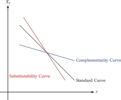
The inclusion of government consumption will affect the slope of the IS curve and will make it flatter in the complementarity case than in the standard case. As a result, the response of output and consumption to changes in interest rates will weaken, indicating a crowding-out effect of fiscal policy on monetary policy. In the substitutability case, on the other hand, the response of the macro variables to changes in interest rates will be higher, as the IS curve becomes steeper than in the standard case. This addition of the fiscal sector makes the model comprehensive to all degrees of substitutability between private and government consumption. It would also overcome the limitations of the ad-hoc approach of including rule-of-thumb consumers.

The results of the paper also show that the fiscal multiplier is sensitive to the strength of the reaction of monetary policy, supporting the theoretical findings of Woodford (2011) and the empirical findings of Koh (2017). Moreover, the results intuitively show that the fiscal multiplier under the complementarity assumption is higher than the substitutability case, similar to the findings of Ercolani and Valle E Azevedo ().

To support the theoretical findings of the paper, we run a fixed panel estimation on 35 OECD countries. The empirical findings show a significant effect of fiscal policy on the transmission mechanism of monetary policy. Where we find that government expenditure has a crowding-in effect on private consumption; positive changes in the policy rate have a negative effect on private consumption; and, most importantly, government consumption dampens the effect of changes in the policy rate on private consumption. These results are robust to the zero lower bound period.

The remainder of the paper is organised as follows: We first demonstrate the structure of our model in the second section. In the third section, we show the parametrisation of the model. The analysis of the impulse response functions is presented in the fourth section. In the fifth section, we illustrate the empirical evidence of the theoretical model. Lastly, the seventh section provides concluding remarks.

2. The model

2.1. Households

Our economy is populated by a representative household that derives utility from aggregate consumption and leisure. The household is assumed to live infinitely, and in each period the household is endowed with one unit of time, divided between work ($N_t$) and leisure ($L_t$): $N_t+L_t=1$. The representative consumer seeks to maximise the following discounted lifetime utility function:

(1) $E_0\sum _{t=0}^{\mathrm{\infty }}{\beta }^{t}U({\bar{C}}_t,N_t)$(1)

The utility function is assumed to be continuous and twice differentiable. $N_t$ is the number of hours worked; $\beta$ is the discount factor; ${\bar{C}}_t$ is the aggregate consumption bundle. $08-07-2020$ is a constant elasticity of substitution aggregate consisting of private consumption $C_t$ and government consumption $G_t$²

(2) ${\bar{C}}_t={\left[{\delta }^{\chi }{C}_t^{1-\chi }+{(1-\delta )}^{\chi }{G}_t^{1-\chi }\right]}^{\frac{1}{1-\chi }}$(2)

where $\delta$ is the share of private consumption in the aggregate consumption bundle, and $08-07-2020$ is the inverse elasticity of substitution between private consumption and government consumption. In this setup, for the government to play a role in the utility function, $\delta$ has to be strictly less than 1. Moreover, the value of $\chi$ has to deviate from 1 in order for government consumption to influence the rest of the dynamics in the model. $C_t$ is the private consumption of goods produced in the economy, and represented by the unit interval: $08-07-2020$ for all $j\in [0,1]$. From Equations (1)(1) $E_0\sum _{t=0}^{\mathrm{\infty }}{\beta }^{t}U({\bar{C}}_t,N_t)$(1) and (2(2) ${\bar{C}}_t={\left[{\delta }^{\chi }{C}_t^{1-\chi }+{(1-\delta )}^{\chi }{G}_t^{1-\chi }\right]}^{\frac{1}{1-\chi }}$(2) ) we can notice that the utility function is non-decreasing in government consumption $G_t$. The above utility function is subject to the following budget constraint:

(3) ${\int }_0^1{P}_t(j)C_t(j)dj+E_t{Q}_{t,t+1}{D}_{t+1}\le D_t+W_t{N}_t+T_t$(3)

where $D_t$ is the nominal payoff at period $t+1$ of bonds held at the end of period t including shares in firms, government bonds and deposits, $W_t$ is wages and $T_t$ is lump-sum transfers to the household net of lump-sum taxes.

The utility function that we use assumes two separabilities. The first one is the separation between consumption and the number of hours worked, and the second one is time separability. The household’s problem is also analysed in two stages in this paper. We first deal with the expenditure minimisation problem faced by the representative household to derive the demand functions for goods. In the second stage, households choose the level of $C_t$ and $N_t$ given the optimally chosen combination of goods.

Now as a first step, the households must minimise their expenditure by optimally choosing the share of each good in the aggregate consumption bundle. Doing so will yield the following demand functions:

(4) $C_t(j)={\left(\frac{P_t(j)}{P_t}\right)}^{-ϵ}{C}_t$(4)

where $P_t\equiv ({\int }_0^1{P}_t(j{)}^{1-ϵ}dj{)}^{\frac{1}{1-ϵ}}$ is the aggregate price index. $ϵ$ is the elasticity of substitution between goods in the economy, and it shows how much the demand for good (j) declines if the relative price of that good increased by 1 unit. A lower elasticity of substitution indicates higher consumption of the good of interest. This assumption shows that goods in the consumption bundle are not perfect substitutes.

Now we turn our attention to the per-period utility function in the following form³

(5) $U(C_t,N_t;G_t)=\frac{{\bar{C}}_t^{1-\sigma }-1}{1-\sigma }-\frac{N_t^{1+\phi }}{1+\phi },$(5)

In the above equation, $\sigma$ is the inverse elasticity of intertemporal substitution. Setting $\sigma$ equal to 1 implies that the household has log-utility in consumption. $\phi$ is the inverse Frisch labour supply coefficient. Parameter $\phi >0$ also measures the curvature of the marginal disutility of labour. The above equation is subject to the aggregate budget constraint, which we get by plugging the above demand bundles and price indices in Equation (3)(3) ${\int }_0^1{P}_t(j)C_t(j)dj+E_t{Q}_{t,t+1}{D}_{t+1}\le D_t+W_t{N}_t+T_t$(3) :

(6) $P_t{C}_t+E_t[Q_{t,t+1}{D}_{t+1}]\le D_t+W_t{N}_t+T_t$(6)

where $E_t$ is the conditional expectation operator. The household’s aggregate expenditure basket is equal to: $P_t{C}_t={\int }_0^1{P}_t(j)C_t(j)dj$. From Equations (5)(5) $U(C_t,N_t;G_t)=\frac{{\bar{C}}_t^{1-\sigma }-1}{1-\sigma }-\frac{N_t^{1+\phi }}{1+\phi },$(5) and (6(6) $P_t{C}_t+E_t[Q_{t,t+1}{D}_{t+1}]\le D_t+W_t{N}_t+T_t$(6) ) we can write the standard optimality condition for the households as follows:

(7) $\frac{W_t}{P_t}=N_t^{\phi }{\bar{C}}_t^{\sigma }{\left(\frac{C_t}{{\bar{C}}_t}\right)}^{\chi }{\delta }^{-\chi }$(7)

The intertemporal optimality condition is:

(8) $\beta {\left(\frac{{\bar{C}}_{t+1}}{{\bar{C}}_t}\right)}^{\chi -\sigma }\left(\frac{P_t}{P_{t+1}}\right){\left(\frac{C_t}{C_{t+1}}\right)}^{\chi }=Q_{t,t+1}$(8)

Taking the conditional expectation of equation ((8)) and rearranging the terms we get:

(9) $\beta R_t{E}_t\left[{\left(\frac{{\bar{C}}_{t+1}}{{\bar{C}}_t}\right)}^{\chi -\sigma }\left(\frac{P_t}{P_{t+1}}\right){\left(\frac{C_t}{C_{t+1}}\right)}^{\chi }\right]=1$(9)

where $R_t=\frac{1}{E_t(Q_{t,t+1})}$ is the one-period return from a riskless bond and $Q_{t,t+1}$ is the expected price of that bond. The form of Equations (7)(7) $\frac{W_t}{P_t}=N_t^{\phi }{\bar{C}}_t^{\sigma }{\left(\frac{C_t}{{\bar{C}}_t}\right)}^{\chi }{\delta }^{-\chi }$(7) and (9(9) $\beta R_t{E}_t\left[{\left(\frac{{\bar{C}}_{t+1}}{{\bar{C}}_t}\right)}^{\chi -\sigma }\left(\frac{P_t}{P_{t+1}}\right){\left(\frac{C_t}{C_{t+1}}\right)}^{\chi }\right]=1$(9) ) deviate from the standard literature, reflecting the inclusion of government consumption in an aggregate CES basket with private consumption in a non-separable form. The first equation depicts labour supply dynamics; it shows labour supply as a function of real wages, given the aggregate consumption bundle and private consumption, and it also shows how the effect of the aggregate consumption bundle on labour supply depends on the value of $\chi$. In the Cobb–Douglas case, when $\chi =\sigma$, the labour supply equation converges to its standard form as government consumption will not affect private consumption. When $\chi >\sigma$, government consumption will have a negative effect on real wages, given its positive effect on labour supply. When $\chi <\sigma$, on the other hand, government consumption will have a positive effect on real wages, given its negative effect on labour supply. The second equation is the Euler equation that characterises consumption smoothing. The Euler equation in this model deviates from the standard form found in the literature. In our case, the smoothing of the aggregate consumption bundle $\bar{C}$ is a component of the above Euler equation. In the Cobb–Douglas case, when $\chi =\sigma$, the above equation would collapse to the canonical version of the Euler equation. When $\chi >\sigma$, any changes in the current value of the aggregate consumption bundle will have a positive effect on private consumption. Conversely, the former will have an adverse effect on private consumption when $\chi <\sigma$.

2.2. The effect of government consumption on private consumption

In this section, we demonstrate how the effect of government consumption on private consumption is subject to the value of the elasticity of substitution between the two. We show this under three different values for the inverse elasticity of substitution between government consumption and private consumption $\chi$: a) The Cobb–Douglas scenario, when the elasticity between government consumption and private consumption is equal to the inverse elasticity of intertemporal substitution $\chi =\sigma$; b) The complementarity case, when $\chi >\sigma$; And c) $\chi <\sigma$, when the two variables are substitutes. Maximising the utility function (5) with respect to the budget constraint (6) yields the first-order condition with respect to private consumption:

(10) $\frac{\mathrm{\partial }\mathrm{\ell }}{\mathrm{\partial }{C}_t}={\delta }^{\chi }{\bar{C}}_t^{-\sigma }{\left(\frac{C_t}{{\bar{C}}_t}\right)}^{-\chi }-P_t{\lambda }_t=0$(10)

To show how the marginal utility of consumption reacts to changes in government consumption under different values of elasticity of substitution, we derive the response of the marginal utility of consumption to changes in $G_t$:

(11) $\frac{\mathrm{\partial }{\lambda }_t}{\mathrm{\partial }{G}_t}=\chi -\sigma {\bar{C}}_t^{\chi -\sigma -1}{\left(\frac{C_t{G}_t}{{\bar{C}}_t}\right)}^{-\chi }\left(\frac{{\delta }^{\chi }{(1-\delta )}^{\chi }}{P_t}\right)$(11)

The above equation shows that the reaction of the marginal utility of consumption for a given level of consumption will depend on the value of $\chi -\sigma$:

1. $\chi =\sigma$: in the Cobb–Douglas case when $\chi =1$, the above ratio will collapse to 0, regardless of the size of $\delta$ in the utility function.

2. $\chi >\sigma$: in this case, the effect of government consumption will be positive, and as $\chi \to \mathrm{\infty }$ the two variables will be perfect complements.

3. $\chi <\sigma$, in this case, the sign of the term above will be negative, and any changes in government consumption will have an adverse effect on private consumption. Also, as $\chi \to 0$, the two variables will be perfect substitutes.

It is easy to see from the above analysis that once we change the size of $\chi$, the dynamics of the whole model will follow, as we will show below. In the separable case when $\chi =\sigma$, the entire model collapses to the standard version of the model since the government consumes different goods than the ones consumed by the representative consumer.

2.3. Firms

2.3.1. Price-setting behaviour

Firms in this model set their prices in a staggered way following Calvo (1983).⁴ Under Calvo contracts, we have a random fraction $1-\theta$ of firms that can reset their prices at period $t$, while the remaining firms, of size $\theta$, keep their prices fixed at the previous period’s price levels. Therefore, ${\theta }^k$ is the probability that a price set at period $t$ will still be valid at period $t+k$. Also, the likelihood of the firm re-optimising its prices will be independent of the time passed since it last re-optimised its prices, and the average duration of prices not to change is $\frac{1}{1-\theta }$. Given the above information, the aggregate price level will take the following form:

(12) $P_t=[\theta (P_{t-1}{)}^{1-ϵ}+(1-\theta )({\bar{P}}_t^{1-ϵ}){]}^{\frac{1}{1-ϵ}}$(12)

where ${\bar{P}}_t$ is the new price set by the optimising firms. From the derivations shown in Appendix B, we get the following form for inflation at period $t$:

(13) ${\mathrm{\Pi }}_t^{1-ϵ}=\theta +(1-\theta ){\left(\frac{{\bar{P}}_t}{P_{t-1}}\right)}^{1-ϵ}$(13)

The above equation shows that the inflation rate at any given period is solely determined by the fraction of firms that reset their prices at that period. In addition, when a given firm in the economy sets its prices, it seeks to maximise the expected discounted value of its stream of profits, conditional that the price it sets remains effective:

(14) $ma{x}_{{\bar{P}}_t}\sum _{k=0}^{\mathrm{\infty }}{\theta }^k{E}_t\{Q_{t,t+k}[c_{jt+k|t}({\bar{P}}_t-{\mathrm{\Psi }}_{t+k})]\}$(14)

The above equation is subject to a sequence of demand constraints: $c_{jt+k}={\left(\frac{{\bar{P}}_t}{P_{t+k}}\right)}^{-ϵ}{C}_t$. Solving this problem (also shown in Appendix B) yields the following optimal decision rule:

(15) $\sum _{k=0}^{\mathrm{\infty }}{\theta }^k{E}_t\left\{Q_{t,t+k}{C}_{t+k}\left[\frac{{\bar{P}}_t}{P_{t-1}}-\mathcal{M}M{C}_{t+k|t}{\mathrm{\Pi }}_{t-1,t+k}^H\right]\right\}=0$(15)

In the above equation, $\mathcal{M}$ is the markup at the steady-state, and $M{C}_t$ is the real marginal cost. As shown in Equation (15)(15) $\sum _{k=0}^{\mathrm{\infty }}{\theta }^k{E}_t\left\{Q_{t,t+k}{C}_{t+k}\left[\frac{{\bar{P}}_t}{P_{t-1}}-\mathcal{M}M{C}_{t+k|t}{\mathrm{\Pi }}_{t-1,t+k}^H\right]\right\}=0$(15) , in the sticky price scheme, producers, given their forward-looking behaviour, adjust their prices at a random period to maximise the expected discounted value of their profits at that period and in the future. Thus, firms in this model will set their prices equal to a markup plus the present value of the future expected stream of their marginal costs. The price-setting behaviour takes this form because firms know that the price they set at period $t$ will remain valid for a random period of time in the future. We also assume that all firms in the economy face the same marginal cost, given the constant returns to scale assumption imposed in the model and the subsidy that the government pays to firms, as shown in the following section. The firms also use the same discount factor $\beta$ as the one used by households, reflecting the fact that households are the shareholders of these firms. All the firms that optimise their prices in any given period will choose the same price, which is also a consequence of the firms facing the same marginal cost. Equation (15)(15) $\sum _{k=0}^{\mathrm{\infty }}{\theta }^k{E}_t\left\{Q_{t,t+k}{C}_{t+k}\left[\frac{{\bar{P}}_t}{P_{t-1}}-\mathcal{M}M{C}_{t+k|t}{\mathrm{\Pi }}_{t-1,t+k}^H\right]\right\}=0$(15) also shows that the inflation rate is proportional to the discounted sum of the future real marginal costs additional to a markup resulting from the monopolistic power of the firms.

2.3.2. Production

A certain firm in the domestic economy produces a differentiated good following a linear production function:

(16) $Y_t(j)=A_t{N}_t(j)$(16)

where $Y_t(j)$ is the output of final good (j) in the home economy, and $A_t$ is the level of technology in the production function. Technology is assumed to be common across all firms in the economy, and it evolves exogenously. $N_t(j)$ is the labour force employed by firm (j). The log form of total factor productivity $a_t=log(A_t)$ is assumed to follow an AR(1) process: $a_t={\rho }_a{a}_{t-1}+{ϵ}_{a,t}$. Where ${\rho }_a$ is the autocorrelation of technology and the innovation to technology ${ϵ}_{a,t}$ has a zero mean and a finite variance ${\sigma }_a$. Capital was excluded from production in this model for the sake of tractability. Aggregate output and aggregate employment in the domestic economy are defined by the Dixit and Stiglitz (1977) aggregator:

(17) $Y_t={\left({\int }_0^1{Y}_t{(j)}^{\frac{ϵ-1}{ϵ}}dj\right)}^{\frac{ϵ}{ϵ-1}};N_t={\left({\int }_0^1{N}_t{(j)}^{\frac{ϵ-1}{ϵ}}dj\right)}^{\frac{ϵ}{ϵ-1}}$(17)

Given the common technology assumption across all firms of the economy, the total cost function for firm (j) is defined as follows:

(18) $T{C}_t(j)=\frac{(1-\tau )W_t{Y}_t(j)}{A_t}$(18)

where $\tau$ is the subsidy that the government gives to firms in order to eliminate the markup distortion, which is created by firms’ monopolistic power. Taking the first-order condition of the above equation yields the following marginal cost equation:

(19) $M{C}_t(j)=\frac{(1-\tau )W_t}{A_t}$(19)

From the above equation, it is clear that the subsidy and the constant return to scale assumption make the marginal cost independent of the firm’s production level. This will make marginal cost common across all firms: $M{C}_t(j)=M{C}_t$, and the common real marginal cost will look like:

(20) $M{C}_t^r=\frac{(1-\tau )}{A_t}\frac{W_t}{P_t}$(20)

The marginal cost equation is expressed in terms of the aggregate price level $P_t$, wages $W_t$, total factor productivity $A_t$, and the subsidy that the government gives to firms ($\tau$). The latter, as explained above, is paid to eliminate the markup distortion created by firms’ monopolistic power.

Lastly, after the aggregation of output and employment, we get the following aggregate production function:

(21) $Y_t=A_t{N}_t$(21)

2.4. Fiscal and monetary policy

2.4.1. Fiscal policy

Government consumption in this paper represents the non-fixed capital formation of government expenditure. For instance, it represents the government provision of goods and services, excluding compensations of state employees. In practice, government consumption could be either a substitute or a complement to private consumption. For instance, government consumption on health and education could crowd-out private consumption on those two items, while government spending on security encourages private consumption in general.

The fiscal sector in this model has the following budget constraint:

(22) $G_t=T_t$(22)

The above equation assumes that government purchases are entirely financed by non-distortionary lump-sum taxes. Noting that in this model we discard the introduction of government debt to avoid redundancy. Following the existing literature,⁵ $G_t$ evolves exogenously according to the following first-order autoregressive process:

(23) $\frac{G_t}{G}={\left\{\frac{G_{t-1}}{G}\right\}}^{{\rho }_g}exp({\zeta }_{G,t})$(23)

where $0<{\rho }_g<1$ is the autocorrelation of government consumption, and ${\zeta }_{G,t}$ represents an i.i.d government consumption shock with constant variance ${\sigma }^2$. Another important feature that we add to this model is to consider that the government consumes from a different market than the one occupied by the private agents. Moreover, following the literature mentioned above, government consumption is produced costlessly.⁶

2.4.2. Monetary policy

The central bank in this model uses a short-term interest rate as its policy tool. In our case, we have a cashless economy where the supply of money is implicitly determined to achieve the interest rate target. We also assume that the central bank will meet all money demand under the policy rate it sets.

We first demonstrate a number of possible policy tools that might be employed by the monetary authority in the economy. The first rule in the model will be the optimal rule:

(24) $\frac{R_t}{R}=\left\{\frac{R{R}_t}{RR}\right\}{\left\{\frac{{\mathrm{\Pi }}_t}{\mathrm{\Pi }}\right\}}^{{\varphi }_{\pi }}{\left\{\frac{Y_t}{Y}\right\}}^{{\varphi }_x}$(24)

The optimal rule illustrates how, by setting domestic CPI inflation and the output gap to zero, the policy rate will equal the natural rate of interest, and it will be able to accommodate developments in the natural rate of output. Thus, the optimal policy reproduces the flexible price equilibrium output, given that the government will pay a subsidy $\tau$ to offset the monopolistic distortion in the economy. The above policy rule will provide a useful benchmark to evaluate the performance of different monetary policy regimes.

The first rule is a Taylor rule:

(25) $\frac{R_t}{R}={\left\{\frac{{\mathrm{\Pi }}_t}{\mathrm{\Pi }}\right\}}^{{\varphi }_{\pi }}{\left\{\frac{Y_t}{Y}\right\}}^{{\varphi }_x}$(25)

The other policy rule is a CPI-targeting Taylor rule:

(26) $\frac{R_t}{R}={\left\{\frac{{\mathrm{\Pi }}_t}{\mathrm{\Pi }}\right\}}^{{\varphi }_{\pi }}$(26)

The parameters of the above policy rules describe the strength of the response of the policy rate to deviations in the variables on the right-hand side. These parameters are also assumed to be non-negative. The last rule is often referred to as a naive interest rule, as it only makes use of observable variables. Also, the inflation response parameter ${\varphi }_{\pi }$ in the above policy rates must be higher than 1 in order for the solution of the model to be unique, as shown by Bullard and Mitra (2002).

2.5. The supply side of the economy

We now turn our attention to the supply side of the economy. From the firm’s section, the log-linearised version of the marginal cost equation of firms in the economy takes the following form:

(27) $\begin{array}{rl}& m{c}_t=-v+w_t-p_t-a_t\\ & =-v+\phi n_t+{\sigma }_{\delta }{c}_t+(\sigma -{\sigma }_{\delta })g_t-a_t\\ & =-v+\phi y_t+{\sigma }_{\delta }{c}_t+(\sigma -{\sigma }_{\delta })g_t-(1+\phi )a_t\\ & =-v+(\phi +{\sigma }_{\delta })y_t+(\sigma -{\sigma }_{\delta })g_t-(1+\phi )a_t\end{array}$(27)

where ${\sigma }_{\delta }=\delta \sigma +(1-\delta )\chi$ is a weighted sum of the intertemporal elasticity of substitution and the elasticity of substitution between government consumption and private consumption. In the above equation, we made use of the log forms of the labour supply equation (Equation 7(7) $\frac{W_t}{P_t}=N_t^{\phi }{\bar{C}}_t^{\sigma }{\left(\frac{C_t}{{\bar{C}}_t}\right)}^{\chi }{\delta }^{-\chi }$(7) ), the production function (Equation 21(21) $Y_t=A_t{N}_t$(21) ), and the market-clearing condition ($c_t=y_t$). The above equation shows the positive effect of the increase in demand on the marginal cost. It also shows that technology has a negative effect on the marginal cost. The effect of government consumption on the marginal cost depends on the value of ${\sigma }_{\delta }$. In the Cobb–Douglas case, government consumption will have no effect on the marginal cost, as ${\sigma }_{\delta }=\sigma$, and the above equation will converge to its standard version. If the inverse elasticity of substitution between government consumption and private consumption is greater than the inverse elasticity of intertemporal substitution ($\chi >\sigma$), the effect of government consumption on the marginal cost is negative, and this is a result of the negative effect of government consumption on real wages in this case. This effect is inherited from the labour supply equation (Equation 7(7) $\frac{W_t}{P_t}=N_t^{\phi }{\bar{C}}_t^{\sigma }{\left(\frac{C_t}{{\bar{C}}_t}\right)}^{\chi }{\delta }^{-\chi }$(7) ) where we show that government consumption has a negative effect on real wages, given the increase in labour supply. On the other hand, when $\chi <\sigma$, government consumption will have a positive effect on the marginal cost, as it positively affects real wages through its negative effect on labour supply. To calculate the natural level of output, we equate the marginal cost to ($-\mu$), which reflects the state of marginal cost under flexible prices.⁷ Getting rid of the constant terms, the natural rate of output equation will be:

(28) ${\bar{y}}_t=-\left(\frac{\sigma -{\sigma }_{\delta }}{\phi +{\sigma }_{\delta }}\right)g_t+\left(\frac{1+\phi }{\phi +{\sigma }_{\delta }}\right)a_t$(28)

The above equation shows the positive effect of government consumption and productivity on the natural rate of output when government consumption is a complement to private consumption. Also, when $\chi >\sigma$, the effect of technology on the natural rate of output is less than its effect on it in the standard case. When government consumption is a substitute to private consumption, however, the effect of government consumption on the natural rate of output will be negative, and the effect of technology will be greater than its effect in the standard case. To get the relationship between the output gap and the marginal cost, we subtract the above equation from Equation (27)(27) $\begin{array}{rl}& m{c}_t=-v+w_t-p_t-a_t\\ & =-v+\phi n_t+{\sigma }_{\delta }{c}_t+(\sigma -{\sigma }_{\delta })g_t-a_t\\ & =-v+\phi y_t+{\sigma }_{\delta }{c}_t+(\sigma -{\sigma }_{\delta })g_t-(1+\phi )a_t\\ & =-v+(\phi +{\sigma }_{\delta })y_t+(\sigma -{\sigma }_{\delta })g_t-(1+\phi )a_t\end{array}$(27) :

(29) $\text{hatm}{c}_t=(\phi +{\sigma }_{\delta })x_t$(29)

where $x_t=y_t-{\bar{y}}_t$ is the output gap. Plugging the value of the marginal cost in the above equation into the derived Phillips curve equation in Appendix B yields inflation as a function of the output gap and inflation expectations one-period ahead:

(30) ${\pi }_t=\beta E_t\{{\pi }_{t+1}\}+\kappa (\phi +{\sigma }_{\delta })x_t$(30)

2.6. The demand side of the economy

Moving to the demand side of the economy, we add the loglinearised form of the Euler equation (Equation 9(9) $\beta R_t{E}_t\left[{\left(\frac{{\bar{C}}_{t+1}}{{\bar{C}}_t}\right)}^{\chi -\sigma }\left(\frac{P_t}{P_{t+1}}\right){\left(\frac{C_t}{C_{t+1}}\right)}^{\chi }\right]=1$(9) ) to the market-clearing equation ($c_t=y_t$) to get:

(31) $y_t=E_t\{y_{t+1}\}-\frac{1}{{\sigma }_{\delta }}[r_t-E_t\{{\pi }_{t+1}\}]+\frac{\sigma -{\sigma }_{\delta }}{{\sigma }_{\delta }}\mathrm{\Delta }{E}_t\{g_{t+1}\}$(31)

In the special case of a Cobb–Douglas utility function, the above IS curve converges back to its canonical representation with the slope being equal to 1. Government consumption when $\chi =\sigma$ has no effect on output as $\sigma ={\sigma }_{\delta }$. In the case of complementarity between government consumption and private consumption $\chi >\sigma$, the slope of the IS curve is flatter than the standard case (Figure 1). The fact that ${\sigma }_{\delta }>1$ when $\chi >\sigma$ dampens the response of output to changes in interest rates. In the case of substitutability between government consumption and private consumption $\chi <\sigma$, the slope of the IS curve is steeper, which strengthens the response of output to changes in interest rates. Also, adding government consumption to the model will shift the IS curve on the right of the standard IS curve. Nevertheless, the new curve will not be parallel to the old curve once we introduce government expenditure to the utility function in a non-separable form. Solving the above IS curve for the output gap yields:

(32) $x_t=E_t\{x_{t+1}\}-\frac{1}{{\sigma }_{\delta }}[r_t-E_t\{{\pi }_{t+1}\}-\bar{r}{r}_t]$(32)

Figure 1. The IS curve.

Where:

(33) $\begin{array}{cc}\bar{r}{r}_t& ={\sigma }_{\delta }\mathrm{\Delta }{y}_{t+1}+(\sigma -{\sigma }_{\delta })\mathrm{\Delta }{g}_{t+1}\\ \hspace{0.17em}& =-\frac{{\sigma }_{\delta }(1-{\rho }_a)(1+\phi )}{\phi +{\sigma }_{\delta }}{a}_t-\frac{(\sigma -{\sigma }_{\delta })(1-{\rho }_g)\phi }{\phi +{\sigma }_{\delta }}{g}_t\end{array}$(33)

The above natural rate of interest still, consistent with the canonical case, negatively reacts to changes in productivity. Nevertheless, the introduction of government consumption in a non-separable form changes the magnitude of the response of the natural rate of interest to a technology shock through the changes in the value of the weighted elasticity of substitution ${\sigma }_{\delta }$. In the complementarity case when $\chi >\sigma$, the response of the natural rate of interest is dampened, given that the slope of the IS curve is flatter in this case. In the substitutability case when $\chi <\sigma$, the response of the natural rate of interest to a technology shock is magnified, given that the IS curve is steeper in this case.

Additionally, when government consumption is included in a non-separable form ($\sigma \ne {\sigma }_{\delta }$), the natural rate of interest reacts to changes in government consumption. In the complementarity case when $\chi >\sigma$, the natural rate of interest positively reacts to changes in government consumption, given the inflationary pressure that the latter causes. In the substitutability case when $\chi <\sigma$, on the other hand, the natural rate of interest negatively reacts to changes in government consumption, given the latter’s negative effect on output.

3. Parametrisation

In the below table, we set $\theta$ equal to 0.75, implying that firms only change their prices once a year. Our discount factor $\beta$ is equal to 0.99. This parameter value implies that, given that $\beta =1/r$ at the steady-state, the annual return is approximately equal to 4%. We set $\phi$ equal to 3, under the assumption that labour supply elasticity is $\frac{1}{3}$. We also set ${\varphi }_{\pi }$ & ${\varphi }_x$ equal to 1.5 and 0.5 following Taylor (1993). We also set the inverse elasticity of substitution between government consumption and private consumption $\chi$ is set equal to 20 following Bouakez and Rebei (2007) and Pieschacon (2012), and we use 0.01 to illustrate the dynamics of the model in the substitutability case. The size of private consumption in the aggregate consumption bundle $\delta$ equal to 0.95. In this regard, and as mentioned above, the weight of $\delta$ hast to be strictly less than 1 for government consumption to influence the dynamics of the model, and different values of $\delta$ between 0 and 1 only affect the model quantitatively. Moreover, changes in the value of $\chi$ do not qualitatively affect the behaviour of the model.

Table

$\beta$	Discount factor	0.99
$\sigma$	inverse elasticity of intertemporal substitution	1
$\phi$	inverse Frisch labour supply elasticity	3
$\chi$	inverse elasticity of substitution between $C_t\text{amp}{G}_t$	20/0.01
$ϵ$	elasticity of substitution	6
$\delta$	share of private consumption in the aggregate consumption bundle	0.95
$\theta$	Calvo probability	0.75
${\rho }_g$	AR(1) coefficient of government expenditure	0.9
${\varphi }_{\pi }$	inflation elasticity of the nominal interest rate	1.5
${\varphi }_x$	output gap elasticity of the nominal interest rate	0.5
${\rho }_a$	AR(1) coefficient of productivity shock	0.9

The inverse elasticity of intertemporal substitution of consumption is set equal to 1, which implies a log-utility form. The elasticity of substitution between the domestically produced goods $ϵ$ equals 6, corresponding to a steady-state markup of 1.2. Also, we adopt the persistence parameter of government consumption ${\rho }_g$ from Gali, Lopez-Salido, and Vallés (2007). As for the standard deviations of the two shock processes, we use the standard deviation of the TFP shock in Galí and Monacelli (2005) ${\sigma }_a=0.0071$, and for the government consumption shock, we use the one in Coenen and Straub (2005) ${\sigma }_g=0.323$.

4. IRF

4.1. The complementarity case

4.1.1. Technology shock

The effect of a technology shock on the output gap and inflation under the optimal policy is zero, by construction. Once the changes in the output gap and inflation are set to zero, the optimal policy rule will follow the path of the natural rate of interest (Equation 33(33) $\begin{array}{cc}\bar{r}{r}_t& ={\sigma }_{\delta }\mathrm{\Delta }{y}_{t+1}+(\sigma -{\sigma }_{\delta })\mathrm{\Delta }{g}_{t+1}\\ \hspace{0.17em}& =-\frac{{\sigma }_{\delta }(1-{\rho }_a)(1+\phi )}{\phi +{\sigma }_{\delta }}{a}_t-\frac{(\sigma -{\sigma }_{\delta })(1-{\rho }_g)\phi }{\phi +{\sigma }_{\delta }}{g}_t\end{array}$(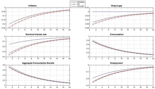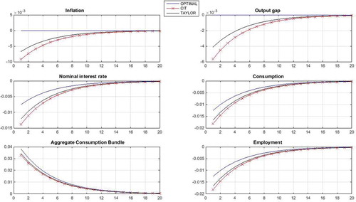33) ). Given that the natural rate of interest takes into account development in the natural rate of output, it will have a neutral monetary stance which is neither expansionary nor contractionary. The above graph shows a persistent reduction in the interest rates, following the technology shock, to support the transitory expansion in output/consumption, and this is consistent with the flexible price case. In this framework, interest rates will only affect the economy via the traditional intertemporal channel in the IS curve. Also, different from the standard case, the natural rate of output and the actual rate of output grow at a rate less than the size of the technology shock. This, in return, causes a decline in employment under the optimal policy rule. If the optimal policy tries to stimulate output to alleviate the decline in employment, it will cause inflationary pressure.

Despite the fact that the nominal values of the other two policy rules are higher than the optimal policy rule, their policy stance, measured by $r_t=i_t-{\pi }_{t+1}$, shows that both policy rules have a contractionary stance, leading to a failure in stimulating the actual rate of output to reach its natural level, and this what causes a negative output gap and negative inflation levels (deflation). This is also a consequence of the inability of the two policies to maintain inflation expectations at the zero level and given the forward-looking behaviour of the agents of the economy. As a result, employment under these two policies falls at a higher rate than under the optimal policy rule, given the relatively higher difference between the growth of output and the size of the technology shock.

Moreover, the effect of the shock on private consumption is identical to its effect on the actual rate of output, given the market-clearing condition of this model. Also, from the above IRF response in Figure 2, it is clear that the Taylor rule outperforms the CPI-targeting Taylor rule. This is attributed to the fact that the earlier keeps track of more variables in the model, and it closely resembles the behaviour of the optimal policy.

Figure 2. Response to a TFP Shock (Complementarity).

4.1.2. Government consumption shock

Under the complementarity assumption, a shock to government consumption will immediately cause an increase in private consumption. The increase in consumption will be mirrored by output, following the market-clearing condition. The effect of the government shock will be positive both on the natural rate of output and the natural rate of interest, as illustrated in Equations (28)(28) ${\bar{y}}_t=-\left(\frac{\sigma -{\sigma }_{\delta }}{\phi +{\sigma }_{\delta }}\right)g_t+\left(\frac{1+\phi }{\phi +{\sigma }_{\delta }}\right)a_t$(28) and (33(33) $\begin{array}{cc}\bar{r}{r}_t& ={\sigma }_{\delta }\mathrm{\Delta }{y}_{t+1}+(\sigma -{\sigma }_{\delta })\mathrm{\Delta }{g}_{t+1}\\ \hspace{0.17em}& =-\frac{{\sigma }_{\delta }(1-{\rho }_a)(1+\phi )}{\phi +{\sigma }_{\delta }}{a}_t-\frac{(\sigma -{\sigma }_{\delta })(1-{\rho }_g)\phi }{\phi +{\sigma }_{\delta }}{g}_t\end{array}$(33) ). We also notice in Figure 3 that the size of the fiscal multiplier is not sensitive to the reaction of monetary policy. This can be seen in the above figure, as consumption and output are not sensitive to the response of different interest rates.

Figure 3. Response to a government consumption shock (Complementarity).

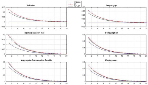
The role of monetary policy under this shock is to control the inflationary increase in demand. Similar to the above analysis, the output gap and inflation are, by construction, set to zero under the optimal policy rule. The policy rule increases in response to a government consumption shock, aiming to reduce the inflationary pressure caused by the shock. Employment under this scenario, since technology is muted, will mirror the behaviour of output.

As for the other two policy rates, despite having nominal values higher than the optimal rule, the policy stance of both rules is expansionary, as their inability to guide inflation expectations to zero levels will weaken the effect of the policy rates on output. As a result, these two policies will fail to mitigate the inflationary pressure of a government consumption shock, and actual output will grow above its natural level, which, in return, will cause an increase in inflation. The Taylor rule still outperforms the CPI-targeting rule under the government consumption shock.

4.2. The substitutability case

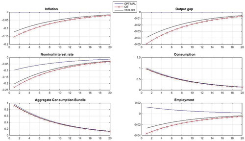
4.2.1. Technology shock

The main difference in the technology shock, in this case, is the response of the optimal policy interest rate. Also, the economy is more sensitive to changes in interest rates, and this makes the required change in the policy rate less than the one under the complementarity case, which is shown in the response of the optimal policy rule in both cases. The effect of a TFP shock on the natural rate of output is greater than the size of the shock itself, as the parameter which governs the relationship between the two is greater than one in the substitutability case. Consequently, this will cause growth in employment above its steady-state level, in order for monetary policy to close the gap between the actual rate of output and its natural level.

Figure 4 illustartes how the reaction of the Taylor rule and the CPI-targeting rule is not different in this case than the complementarity case. Both rules take a contractionary stance, despite the fact that their nominal values are lower than the optimal rule, a result from their inability to manage expectations. This, in return, will cause a negative output gap, and this will cause deflation and a drop in employment.

Figure 4. Response to a TFP Shock (Substitutability).

4.2.2. Government consumption shock

Under the substitutability assumption, a shock in government consumption will immediately cause a decline in private consumption, as shown below in Figure 5. The drop in output and employment will be identical to the drop in consumption given the market-clearing condition and the production function, respectively. Additionally, the effect of government consumption on the natural rate of output and the natural rate of interest will be adverse, also consistent with the substitutability assumption between government consumption and private consumption.

Figure 5. Response to a government consumption shock (Substitutability).

In this case, the role of monetary policy is to lessen the adverse effect of government consumption on the economy. Under the optimal policy rule, the output gap and inflation are set to zero, by construction. The decline in the policy rule will help in mitigating the drop in output and consumption, caused by the increase in government consumption. Similar to the complementarity case, the fiscal multiplier, in this case, will not be sensitive to the reaction of monetary policy.

The Taylor rule and the CPI-targeting rule take a contractionary monetary stance, resulting from their inability to guide inflation expectations to zero levels, and this will weaken the effect of the policy rates on output. This will cause the actual rate of output to decline and in return, a drop in employment. The Taylor rule still outperforms the CPI-targeting rule under this government consumption shock, similar to all the above simulations.

4.3. Monetary shock

In this section, we show how the introduction of government consumption affects the transmission mechanism of monetary policy. We do this by comparing the effect of a monetary policy shock both under the complementarity assumption and under the substitutability assumption. We use the Taylor rule (Equation 25(25) $\frac{R_t}{R}={\left\{\frac{{\mathrm{\Pi }}_t}{\mathrm{\Pi }}\right\}}^{{\varphi }_{\pi }}{\left\{\frac{Y_t}{Y}\right\}}^{{\varphi }_x}$(25) ) for this exercise by adding an exogenous component ${ϵ}_{r,t}$ to the rule, and this shock represents an i.i.d monetary policy shock with constant variance ${\sigma }_r^2$. A one standard deviation of a monetary shock has a contractionary effect on the economy, as it will depress output and pushes price downwards. Monetary policy will not have an effect on the natural rate of interest and the natural rate of output.

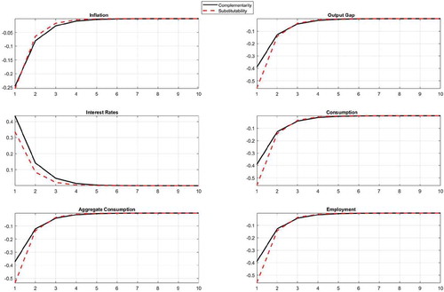
Figure 6 shows that an increase in the policy rate depresses output. The decline in output pushes prices downwards (deflation) and the decline in output is mirrored by a drop in consumption and employment, following the market-clearing condition and the production function, respectively. The above figure mainly shows that the effect of monetary policy is higher under the substitutability assumption than under the complementarity assumption. All of the central macroeconomic variables are more affected by the monetary shock when government consumption is a substitute for private consumption. The only exception is the behaviour of interest rates. This is attributed to the endogenous changes in interest rates which are induced by the output gap and inflation. The results mainly support the paper’s claim that government consumption has a crowding-out effect on monetary policy when it has a crowding-in effect on private consumption and vice versa.

Figure 6. Response to a monetary shock.

5. Empirical evidence: panel fixed effects estimates

The above theoretical model clearly illustrates the crowding-out effect of government consumption to monetary policy when the former has a crowding-in effect on private consumption and vice versa. This section empirically tests the hypothesis mentioned above by adopting a panel fixed-effect model.

We first start by running panel regressions that try to explain the effect of government consumption and monetary policy on private consumption. We then include an interaction variable measure of government consumption and the policy rate. We specify a variety of empirical models to assess the robustness of the results. As shown below, the results display that government consumption dampens the effect of monetary policy when it has a crowding-in effect on government consumption. The specification of the model takes the following form:

(34) $C_c=\alpha +({\beta }_1+{\beta }_2{G}_c)\mathrm{\Delta }{i}_{it}^p+{\beta }_3{G}_c+{\beta }_4{Y}_c+{\beta }_5{Y}_{HP}+{\beta }_6{C}_{HP}+{\beta }_7{D}_1$(34)

where $C_c$ is cyclical private consumption, $G_c$ is cyclical government consumption and $Y_c$ is cyclical output. $Y_{HP}$ and $C_{HP}$ are the trend components of output and private consumption, respectively. $D1$ is a dummy variable that accounts for the zero lower bound period (2008q1-2013q4).

The analysis is conducted on 35 OECD countries (excluding Turkey). As mentioned above, private consumption, government consumption and output are detrended. We also control for trend private consumption and output. The data for these three variables come from the OECD database. All variables are expressed in real terms. Also, data on interest rates come from the IMF IFS database, and it is expressed in nominal terms. The data is in quarterly frequency, and it covers the period 1995q1 – 2017q4.

The results of all the panel regressions are shown in Table 1. The first specification shows how government consumption has a crowding-in effect on private consumption. The results show that a 10% increase in government consumption causes a contemporaneous and statistically significant increase of 1.14% in private consumption. The size of this effect is robust through all specifications of the above table. Starting from the second specification, we add the policy interest rate, which represents the monetary policy instrument. The results show an adverse, significant effect of the policy rate on private consumption in the second and third specifications.

Table 1. The crowding-out effect of monetary policy to monetary policy.

Dependent variable:
Private Consumption	(1)	(2)	(3)	(4)	(5)	(6)
Government Consumption	0.114***	0.123**	0.126***	0.114***	0.124***	0.126***
	(0.016)	(0.016)	(0.016)	(0.016)	(0.016)	(0.016)
Changes in Policy Rate		−0.0004**	−0.0004**		−0.0004**	−0.0004**
		(0.0002)	(0.0002)		(0.0002)	(0.0002)
Changes in Policy Rate x			0.0001**			0.0001**
Government Consumption			(0.00006)			(0.00007)
Output	0.741***	0.744***	0.747***	0.741***	0.744***	0.746***
	(0.013)	(0.013)	(0.013)	(0.013)	(0.013)	(0.013)
Trend Consumption	0.0284***	0.0297***	0.0304***	0.0284**	0.0298***	0.0305***
	(0.006)	(0.006)	(0.006)	(0.006)	(0.006)	(0.006)
Trend Output	−0.0264***	−0.0294***	−0.0301***	−0.0263***	−0.0291***	−0.0301***
	(0.006)	(0.006)	(0.006)	(0.006)	(0.006)	(0.006)
Financial Crisis Dummy				−0.008	−0.009	−0.006
				(0.060)	(0.059)	(0.059)
Constant	−0.890	1.061	1.511	−0.983	0.956	1.439
	(1.692)	(1.701)	(1.739)	(1.820)	(1.828)	(1.865)
Country Fixed Effects	yes	yes	yes	yes	yes	yes
Observations	3,220	3,150	3,185	3,220	3,185	3,150
Countries	35	35	35	35	35	35
R-squared	0.47	0.51	0.51	0.47	0.50	0.50

Standard errors are in parentheses.

Significance levels: *** p < 0.01, ** p < 0.05, * p < 0.1.

In the third specification, we add an interaction variable between government consumption and the policy rate. Despite the fact that the coefficient of the policy rate (${\beta }_1$) remains unchanged, (${\beta }_2$) shows the crowding-out effect of government consumption on monetary policy. After adding the interaction term, the combined effect (${\beta }_1+{\beta }_2$) shows a decline in the effect of the policy rate on consumption from −0.0004 to −0.0003, supporting the predictions of the above theoretical model.

In the last three specifications, and since the estimation period covers the zero lower bound period, we add a dummy variable that accounts for the zero lower bound period. The results of all three specifications show that the estimated relationships of the model are robust to the zero lower bound period. Moreover, the financial crisis dummy variable, despite showing a negative effect on private consumption, is not statistically significant across the last three specifications.

6. Conclusion

How does the inclusion of government consumption in the utility function affect the dynamics of a standard New Keynesian model? And how does government consumption affect the transmission mechanism of monetary policy? To address these questions, we developed a standard New Keynesian model which incorporates meaningful government consumption in the utility function in a non-separable form. The inclusion of the fiscal sector to the model gives us a more insightful analysis of the dynamics of the model.

The introduction of government consumption to the utility function in a non-separable form will affect the slope of the IS curve as it will make it flatter in the complementarity case between government consumption and private consumption. As a result, the response of output to changes in the interest rates will weaken, showing an indication of a crowding-out effect of fiscal policy towards monetary policy. When government consumption and private consumption are substitutes, the response of output to changes in interest rates will be higher than both the traditional and the complementarity case. Failure to account for the presence of the fiscal sector will result in deflationary pressure in case of a technology (supply) shock and inflationary pressure in case of government consumption (demand) shock when government consumption is a complement to private consumption. In the substitutability case, the two shocks will cause deflationary pressure if the presence of government consumption is not taken into account.

The effect of the interest rate in this economy transmits through the traditional intertemporal channel in the IS curve. Different to the response to a TFP shock under the optimal policy response in the canonical version of the model, the output will not grow at an equivalent rate to the technology shock in this model. In the complementarity case, employment will drop, and if monetary policy tries to stimulate output to alleviate the decline in employment, it will cause inflationary pressure. In the substitutability case, a TFP shock will cause an increase in employment above its steady-state level. This results from the size of the parameter that governs the relationship between technology and the natural rate of output, which is larger than the one in the standard case.

Moreover, the effect of monetary policy is higher under the substitutability assumption than under the complementarity assumption, and all of the central macroeconomic variables are more sensitive to a monetary shock when government consumption is a substitute to private consumption. These results show that when government consumption has a crowding-out effect on monetary policy, it has a crowding-in effect on private consumption and vice versa. We also find that the reaction of monetary policy does not affect the fiscal multiplier in the economy under the structure of this model.

Our empirical results support the effect of fiscal policy on the transmission mechanism of monetary policy. Running a panel estimation on 35 OCED countries, we find that government expenditure has a crowding-in effect on private consumption, positive changes in the policy rate have a negative effect on private consumption and, most importantly, government consumption dampens the effect of changes in the policy rate on private consumption. These results are robust to the zero lower bound period.

In this paper, government consumption was assumed to be exogenous, and the setting of the model was in a closed economy framework. Developing the current setting to an open economy model would provide more insight into the dynamics of the model regarding developments in the internal balances versus external balance framework. Also, the current framework could be further developed into a two-country framework, and the spillover effect could be studied with the introduction of non-separable government consumption. Another possible extension to this model is to add government investment to produce capital. This capital could be rented to firms as the only available capital in the economy so that it could be a complement to the other factors of production. On the other hand, public capital could be included as a substitute for private capital.

Disclosure statement

No potential conflict of interest was reported by the author.

Additional information

Notes on contributors

Haytem Troug

Haytem Troug is a senior economist at the Central Bank of Libya. Prior to his work at the central bank, he worked with several multinational institutions, such as UNDP and the African development bank. Mr. Troug hold a doctorate degree from the university of Exeter.

Notes

¹ The literature has yet to reach consensus on the effect of government consumption on private consumption. While Bouakez and Rebei (2007), Pieschacon (2012), and Gali et al. (2007) show a crowding-in effect of government on private consumption, Ganelli (2003) and Ercolani and E Azevedo (2014) show a crowding-out effect. Barro (1990) and Barro and Sala-i Martin (1992), on the other hand, show that the effect of government expenditure is conditional on the type of expenditure and the levied taxes. The disparity in the literature goes beyond the theoretical models, where even empirical models show different estimates depending on the modelled period and the adopted estimation method.

² The inclusion of government consumption in the utility function, despite being understudied, as highlighted by Cantore, Levine, and Melina (2014), seems appealing since agents gain utility from government consumption, making the introduction of government consumption meaningful in the model. The inclusion is also supported by the fact that the primary purpose of government consumption in any economy is to provide goods services for the agents of that economy. Also, government consumption in this framework can be thought of as a public good that households consume at free cost, e.g, government expenditure on security and defence which stimulates private consumption and increases the utility of households.:

³ We replaced private consumption in the utility function with the aggregate consumption bundle. As noted above, this is one of the deviations that we make from Gali (2008).:

⁴ The Calvo model makes aggregation easier because it gets rid of the heterogeneity in the economy. The alternative pricing scheme is the quadratic cost of price adjustment by Rotemberg (1982). The two dynamics are equivalent up to a first-order approximation.

⁵ See, for example, Bouakez and Rebei (2007) ^and Sims and Wolff (2018)^.

⁶ Despite the fact that the assumption of costless government consumption is counterintuitive, it suits the purpose of this paper to focus on how the non-fiscal sectors react to different shocks once government consumption is introduced in a non-separable format.

⁷ $\mu$ = 0 in the perfect competition case.

⁸ Log-linearising around a steady state of zero inflation allows us to get rid of the price dispersion created by the nominal friction in the model.

Appendix A

Log-linearisation

• Aggregate consumption bundle:

(35) ${\bar{c}}_t=\delta c_t+(1-\delta )g_t$(35)

• IS curve:

(36) $x_t=E_t\{x_{t+1}\}-\frac{1}{{\sigma }_{\delta }}[r_t-E_t\{{\pi }_{t+1}\}-\bar{r}{r}_t]$(36)

• Natural rate of interest:

(37) $\bar{r}{r}_t=-\frac{{\sigma }_{\delta }(1-{\rho }_a)(1+\phi )}{\phi +{\sigma }_{\delta }}{a}_t+-\frac{((\sigma -{\sigma }_{\delta })(1-{\rho }_g)\phi }{\phi +{\sigma }_{\delta }}{g}_t$(37)

• Phillips curve:

(38) ${\pi }_t=\beta E_t\{{\pi }_{t+1}\}+\kappa (\phi +{\sigma }_{\delta })x_t$(38)

• Flexible-price output:

(39) ${\bar{y}}_t=-\left(\frac{\sigma -{\sigma }_{\delta }}{\phi +{\sigma }_{\delta }}\right)g_t+\left(\frac{1+\phi }{\phi +{\sigma }_{\delta }}\right)a_t$(39)

• Output gap:

(40) $x_t=y_t-{\bar{y}}_t.$(40)

• Production function:

(41) $y_t=a_t+n_t.$(41)

• Labour supply:

(42) $w_t-p_t=\phi n_t+{\sigma }_{\delta }{c}_t+(\sigma -{\sigma }_{\delta })g_t.$(42)

• Monetary policy:

(43) $\left\{\begin{array}{cc}{r}_t=\overline{r{r}_t}+{\varphi }_{\pi }{\pi }_t+{\varphi }_x{x}_t,& \mathrm{O}\mathrm{p}\mathrm{t}\mathrm{i}\mathrm{m}\mathrm{a}\mathrm{l}\mathrm{p}\mathrm{o}\mathrm{l}\mathrm{i}\mathrm{c}\mathrm{y},\\ r_t={\varphi }_{\pi }{\pi }_t+{\varphi }_x{x}_t,& \mathrm{T}\mathrm{a}\mathrm{y}\mathrm{l}\mathrm{o}\mathrm{r}\mathrm{r}\mathrm{u}\mathrm{l}\mathrm{e},\\ r_t=\rho +{\varphi }_{\pi }{\pi }_t,& \mathrm{C}\mathrm{P}\mathrm{I}\mathrm{i}\mathrm{n}\mathrm{f}\mathrm{l}\mathrm{a}\mathrm{t}\mathrm{i}\mathrm{o}\mathrm{n}\mathrm{t}\mathrm{a}\mathrm{r}\mathrm{g}\mathrm{e}\mathrm{t}\mathrm{i}\mathrm{n}\mathrm{g},\end{array}\right.$(43)

• Market-clearing condition:

(44) $y_t=c_t$(44)

• Exogenous process:

(45) $a_t={\rho }_a{a}_{t-1}+{ϵ}_{a,t},$(45)

(46) $g_t={\rho }_g{g}_{t-1}+{ϵ}_{g,t}.$(46)

Appendix B

To understand the inflation dynamics in the model, we start by analysing the price-setting behaviour of firms. We follow the steps of GM2005, and the third chapter of Gali2008 to derive the price-setting behaviour of firms in the model under a sticky price framework. The aggregate domestic price index in the model is a weighted average of prices that have been adjusted at period $t$ and prices that have not been adjusted:

(47) $P_t=[\theta (P_{t-1}{)}^{1-ϵ}+(1-\theta )({\bar{P}}_t{)}^{1-ϵ}{]}^{\frac{1}{1-ϵ}}$(47)

${\bar{P}}_t$ is the re-optimised price that a fraction of the firms $(1-\theta )$ chooses at period $t$, and this is normally higher than the prevailing price during the last period before. $P_{t-1}$ is the price imposed by the other fraction of firms who have not been able to adjust their prices, and this is why we keep last period’s prices as the prevailing prices for those firms. We divide the above equation by $P_{t-1}$ to get:

(48) ${\mathrm{\Pi }}_t^{1-ϵ}=\theta +(1-\theta )(\frac{{\bar{P}}_t}{P_{t-1}}{)}^{1-ϵ}$(48)

Log-linearising the above equation around a steady state with zero-inflation yields⁸

(49) ${\pi }_t=(1-\theta )({\bar{p}}_t-p_{t-1})$(49)

In the above equation, inflation at the current period is affected by the price adjustment that a fraction of the firms in the economy makes to their prices. Therefore, as mentioned above, we start deriving the price-setting behaviour of firms to capture the dynamics of prices in the economy. When firms set their prices according to Calvo83 contract scheme, they aim to maximise the expected discounted value of their profits under the assumption that the newly set price will still be effective:

(50) $ma{x}_{{\bar{P}}_t}\sum _{k=0}^{\mathrm{\infty }}{\theta }^k{E}_t\{Q_{t,t+k}[c_{jt+k|t}({\bar{P}}_t-{\mathrm{\Psi }}_{t+k})]\}$(50)

$\mathrm{\Psi }$ is the cost function, ${\theta }^k$ is the probability that the re-optimised price at period t will remain effective at period t + k, and $Q_{t,t+k}$ is the discount factor of nominal pay off and it is defined in equation (9)(9) $\beta R_t{E}_t\left[{\left(\frac{{\bar{C}}_{t+1}}{{\bar{C}}_t}\right)}^{\chi -\sigma }\left(\frac{P_t}{P_{t+1}}\right){\left(\frac{C_t}{C_{t+1}}\right)}^{\chi }\right]=1$(9) . $c_{jt+k|t}$ is the Expected demand/production for period t + k at period t. The equation is subject to the following demand constraint: $c_{jt+k}={\left(\frac{{\bar{P}}_t}{P_{t+k}}\right)}^{-ϵ}{C}_t$. Plugging in the demand function into the firm’s maximisation problem yields:

(51) $ma{x}_{{\bar{P}}_t}\sum _{k=0}^{\mathrm{\infty }}{\theta }^k{E}_t\{Q_{t,t+k}[{\left(\frac{{\bar{P}}_t}{P_{t+k}}\right)}^{-ϵ}{C}_{t+k}({\bar{P}}_t-{\mathrm{\Psi }}_{t+k})]\}$(51)

Taking the first-order condition of the above equation yields:

(52) $\sum _{k=0}^{\mathrm{\infty }}{\theta }^k{E}_t\{Q_{t,t+k}{C}_{t+k}[{\bar{P}}_t-\mathcal{M}{\psi }_{t+k|t}]\}=0$(52)

$\psi$ is the nominal marginal cost, and $\mathcal{M}$ is the gross mark-up and is equal to $\frac{ϵ}{ϵ-1}$. Now, we divide the above equation by $P_{H,t-1}$ and divide and multiply the second term by $P_{H,t+k}$:

(53) $\sum _{k=0}^{\mathrm{\infty }}{\theta }^k{E}_t\left\{Q_{t,t+k}{C}_{t+k}\left[\frac{{\bar{P}}_{H,t}}{P_{H,t-1}}-\mathcal{M}M{C}_{t+k|t}{\mathrm{\Pi }}_{t-1,t+k}^H\right]\right\}=0$(53)

Where ${\mathrm{\Pi }}_{t-1,t+k}^H=\frac{P_{H,t+k}}{P_{H,t-1}}$, and $M{C}_{t+k|t}=\frac{{\psi }_{t+k|t}}{P_{H,t+k}}$. We log-linearise the above equation around a zero-inflation steady state. Noting that $Q_{t,t+k}$ in the steady state will equal ${\beta }^k$:

(54) ${\bar{p}}_t-p_{t-1}=(1-\beta \theta )\sum _{k=0}^{\mathrm{\infty }}(\beta \theta {)}^k{E}_t\{m{c}_{t+k|t}+\mu +(p_{t+k}-p_{t-1})\}$(54)

We notice from the above equation that the firms discount the expected stream of their future profits using the household’s discount factor. This is simply attributed to the fact that the households are the shareholders of those firms. Rearranging the above equation gives:

(55) ${\bar{p}}_t=\mu +(1-\beta \theta )\sum _{k=0}^{\mathrm{\infty }}(\beta \theta {)}^k{E}_t\{m{c}_{t+k|t}+p_{t+k}\}$(55)

The above equation is describing how the firm set their prices with a certain mark-up and the discounted present value of the stream of marginal costs, and it is the one we use in the text. In the case when $\theta =0$, all firms will be able to adjust their prices in each period (flexible price scheme), and the above equation will simplify to:

(56) ${\bar{p}}_t=\mu +m{c}_t$(56)

The price the firms set in this case is equal to their markup over the nominal marginal cost. Of course, this shows that the price set by the firms is above their marginal cost since the markup is greater than 1. As a result, the output will be lower than its level under perfect competition. It will be shown how the government can offset this distortion by giving the firms a certain employment subsidy. Now going back to equation (54)(54) ${\bar{p}}_t-p_{t-1}=(1-\beta \theta )\sum _{k=0}^{\mathrm{\infty }}(\beta \theta {)}^k{E}_t\{m{c}_{t+k|t}+\mu +(p_{t+k}-p_{t-1})\}$(54) , if we rewrite down the equation in a compact form we get:

(57) ${\bar{p}}_t-p_{t-1}=\beta \theta E_t\{p_{t+1}-p_t\}+{\pi }_t+(1-\beta \theta )\text{hatm}{c}_t$(57)

Where $\text{hatm}{c}_t=m{c}_t-p_t+\mu$. Adding the above equation to the price-setting equation gives us:

(58) ${\pi }_t=\beta E_t\{{\pi }_{t+1}\}+\kappa \text{hatm}{c}_t$(58)

Where $\kappa =\frac{(1-\theta )(1-\beta \theta )}{\theta }$. The above equation is the core New Keynesian Phillips Curve. We develop it in the text to link inflation to the output gap through the relationship between the $\hat{m}c$ and the output gap $(x_t)$. $\kappa$ in the Phillips curve equation is strictly decreasing in the stickiness parameter $\theta$. From the above equation, we see that inflation in this type of models is a result of aggregate price-setting of the firms who adjust their prices based on current and future stream of their marginal costs.

References

- Barro, R. (1990). Government spending in a simple model of endogenous growth. Journal of Political Economy, 98(5, Part 2), S103–S126.
- Barro, R., & Sala-i Martin, X. (1992). Public finance in models of economic growth. Review of Economic Studies, 59(4), 645–661.
- Baxter, M., & King, R. G. (1993). Fiscal policy in general equilibrium. The American Economic Review, 83(3), 315–334.
- Bouakez, H., & Rebei, N. (2007). Why does private consumption rise after a government spending shock? (pourquoi est-ce que la consommation privée augmente après un choc de dépenses gouvernementales?). The Canadian Journal of Economics/Revue Canadienne d’Economique, 40(3), 954–979.
- Bullard, J., & Mitra, K. (2002). Learning about monetary policy rules. Journal of Monetary Economics, 49(6), 1105–1129.
- Calvo, G. A. (1983). Staggered prices in a utility-maximizing framework. Journal of Monetary Economics, 12(3), 383–398.
- Cantore, C., Levine, P., & Melina, G. (2014). On habit and utility-enhancing government consumption [Discussion Paper Series 14/06].
- Christiano, L., Eichenbaum, M., & Rebelo, S. (2011). When is the government spending multiplier large? Journal of Political Economy, 119(1), 78–121.
- Coenen, G., & Straub, R. (2005). Does government spending crowd in private consumption? Theory and empirical evidence for the euro area*. International Finance, 8(3), 435–470.
- Cogan, J. F., Cwik, T., Taylor, J., & Wieland, V. (2010). New keynesian versus old Keynesian government spending multipliers. Journal of Economic Dynamics and Control, 34(3), 281–295.
- Davig, T., & Leeper, E. (2011). Monetary-fiscal policy interactions and fiscal stimulus. European Economic Review, 55(2), 211–227.
- Dixit, A., & Stiglitz, J. (1977). Monopolistic competition and optimum product diversity. American Economic Review, 67(3), 297–308.
- Eggertsson, G. (2011). What fiscal policy is effective at zero interest rates? (Tech. Rep.).
- Ercolani, V., & E Azevedo, J. V. (2014). The effects of public spending externalities. Journal of Economic Dynamics and Control, 46, 173–199.
- Gali, J. (2008). Introduction to monetary policy, inflation, and the business cycle: An introduction to the new keynesian framework.
- Gali, J., Lopez-Salido, D., & Vallés, J. (2007). Understanding the effects of government spending on consumption. Journal of the European Economic Association, 5(1), 227–270.
- Gali, J., & Monacelli, T. (2008). Optimal monetary and fiscal policy in a currency union. Journal of International Economics, 76(1), 116–132.
- Galí, J., & Monacelli, T. (2005). Monetary policy and exchange rate volatility in a small open economy. Review of Economic Studies, 72(3), 707–734.
- Ganelli, G. (2003). Useful government spending, direct crowding-out and fiscal policy interdependence. Journal of International Money and Finance, 22(1), 87–103.
- Koh, W. C. (2017). Fiscal multipliers: New evidence from a large panel of countries. Oxford Economic Papers, 69(3), 569–590.
- Obstfeld, M., & Rogoff, K. (1995). Exchange rate dynamics redux. Journal of Political Economy, 103(3), 624–660.
- Obstfeld, M., & Rogoff, K. (1996). Foundations of international macroeconomics (Vol. 1, 1st ed.). The MIT Press.
- Pieschacon, A. (2012). The value of fiscal discipline for oil-exporting countries. Journal of Monetary Economics, 59(3), 250–268.
- Rotemberg, J. (1982). Sticky prices in the united states. Journal of Political Economy, 90(6), 1187–1211.
- Sims, E., & Wolff, J. (2018). The output and welfare effects pf government spending shocks over the business cycle. International Economic Review, 59(3), 1403–1435.
- Smets, F., & Wouters, R. (2007). Shocks and frictions in us business cycles: A bayesian dsge approach. American Economic Review, 97(3), 586–606.
- Taylor, J. B. (1993). Discretion versus policy rules in practice. Carnegie-Rochester Conference Series on Public Policy, 39, 195–214.
- Woodford, M. (2011). Simple analytics of the government expenditure multiplier. American Economic Journal: Macroeconomics, 3(1), 1–35.