Dynamic forecasting of banking crises with a Qual VAR

ABSTRACT

This paper applies a Qual VAR approach to generate a continuous banking crisis indicator from an underlying latent variable using a Markov Chain Monte Carlo algorithm. Four decades of banking crises are assessed by accounting for the evolutionary nature of precursors, as measured through periodic, regional, and developmental effects using a representative sample of countries. Aggregate results from forecast error variance decomposition show that banking sector variables explain nearly half of total variation, external sector a third and real sector a fifth. Findings suggest that recursive out-of-sample forecasts up to 12-months preceding a banking crisis render vital early warning signals, and as based on quarterly data, support expeditious response times. In out-of-sample forecasting, the Qual VAR outperforms a probit model. Improved forecasting performance may assist banking oversight departments and support remediation efforts of policymakers to adequately and timeously respond to banking crises.

KEYWORDS:

• Qual VAR
• Markov Chain Monte Carlo
• latent variable
• banking crises
• leading indicators
• forecasting
• early warning signal

1. Introduction

The severe ramifications of the recent Global Financial Crisis have renewed interest in the perennial nature of banking crises. Finding the manifestations of banking frailties to be a recurring phenomenon, Reinhart and Rogoff (2009) also solidify its exemptive characteristics in comparison to traditional financial crises, pointing out that it remains agnostic to level of economic development. Faltering growth in the aftermath of broad-based liquidity contractions directly impacts socioeconomic development and political dispositions, with fiscal costs equivalent to 12 percent and 23 percent of gross domestic product for respectively developed economies and emerging markets (Laeven & Valencia, 2018).

Research on banking crises underscore a continuum of precursors. Highlighted in Online Appendix B1, insolvencies can stem from macroeconomic imbalances, deregulation, financial innovation, and inadequate regulatory oversight. A moot consideration of the recent Global Financial Crisis centers on the repeated experience of banking sector weaknesses observed in a range of countries, however, distinguished from comparable yet unaffected economies. While precursors to banking crises are in some instances uniform, a strengthened banking sector and solid macroeconomic environment arguably supported developed economies such as Japan and Australia and emerging markets including Mexico, Thailand and Poland to remain resilient while neighboring countries succumbed to asset frailties.

Crisis prevention should be the fulcrum of economic researchers. Lacking a proverbial canary in a coal mine due to the bounded accuracy of economic forecasting tools, and the dire need for prescient knowledge, necessitate proficient enhancements to econometric models and the development of new and hybrid methodologies to meticulously assess underlying real and banking sector vulnerabilities. In pursuit of supporting macroprudential policy and economic discourse, necessary to expose incredulity and hubris, a balanced yet introspective approach to gain credence is imperative.

To contribute to the literature on banking sector vulnerabilities in general and crisis prevention in particular, this paper introduces an emerging methodology in the investigation of banking crises. In this regard, the econometric approach is a Qualitative Vector Autoregression (Qual VAR), which encompasses qualitative information and is centered on a binary choice variable, in pursuit of detecting the probability of a banking crisis or tranquil period. The benefits of using Qual VAR include explicit accounting of the endogenous nature of banking crises and through impulse responses provide a valuable measurement of the dynamic effects of a banking crisis on the economy.

To examine universal applicability, the study draws on 40 years of banking crises, comprising a total sample of 18 countries which experienced a combined 34 crises between 1971 and 2016. To account for periodic, regional and developmental effects, episodes are assessed across representative observations. Substantiated through literature studies on leading indicators of banking crises, explanatory variables represent real, banking and external sectors, including gross domestic product, investment, consumption, inflation, interest rates, banking assets and liabilities, exchange rates, terms of trade, reserves and exports.

Results from forecast error variance decomposition solidify the importance of banking sector variables as leading indicators, in addition to external and real sectors. For 11 of the 18 countries, the banking sector's contribution exceeds 40 percent. In the case of some countries, a limited count of specific variables provides the bulk of the impact, necessitating ringfenced macroprudential focus areas.

Findings on predictive power suggest that recursive out-of-sample forecasts up to 12-months preceding a banking crisis render notable results for most countries across quintessential categories, reasoning a compelling case for unremittent monitoring and evaluation of underlying banking sector frailties. In rendering a continuous banking crisis indicator, the Qual VAR modeling framework allows expeditious response times which provide macroprudential policymakers and oversight departments with a scientific and objective toolkit supporting enhanced preparations.

The structure of the paper is as follows. Section 2 provides an overview of the empirical literature. Section 3 explains the econometric methodology. Section 4 describes the data and variable selection and Section 5 evaluates the findings. Section 6 concludes.

2. Empirical literature

2.1. Forecasting tools

Manifesting as a low-frequency high impact event, the debilitating experience of the recent Global Financial Crisis argues a compelling case for a review of the performance of available forecasting tools. Hence, renewed interest in econometric and non-parametric methodologies spanning currency, balance of payments, debt, and banking crises concentrate on its applicability to crises prognostication.

Kaminsky, Lizondo, and Reinhart (1998) introduced the signals approach to serve as early warning alarm for subsequent crises, which was based on a set of key indicators exceeding threshold levels. Applications include asset price bubbles (Alessi & Detken, 2011) and sovereign debt crises (Knedlik & Von Schweinitz, 2012).

Frankel and Rose (1996) developed binary choice models such as probit and logit models, which are frequently applied by the private sector, public sector, and international financial institutions for a diverse spectrum of early warning signals. Multivariate probit or logit models are commonly used by private sector analysts to determine the likelihood of an ensuing currency crisis, usually, one to three months in advance, particularly as it impacts on currency, hedging, and futures trading strategies. Demirgüç-Kunt and Detragiache (2000), Bussière and Fratzscher (2006) and Barrell, Davis, Karim, and Liadze (2010) examine binary logistic regression performance in the context of various financial crises. Reviews of these models have generally highlighted mixed results as out-of-sample forecasts generated too few crisis signals or too many false signals to be labelled accurate for policy making (Berg, Borensztein, & Pattillo, 2005; Frankel & Saravelos, 2012). Rudebusch and Williams (2009), Chauvet and Potter (2010) and Nyberg (2010) focus on identifying business cycle turning points. In the context of binary choice models, which is a construct based on an assumed latent time series variable, a salient critique centers on its inability to representatively capture and convey the underlying time series element of the macroeconomic data on which the constructed binary variable is dependent (Harding & Pagan, 2011).

To capture the time series element inherent in macroeconomic applications, Regime Switching models can be used, which also allow non-linear modelling. For this quantitative modelling technique, models have been used over an extensive period stretching as far as Quandt (1958), Goldfeld and Quandt (1973) and Hamilton (1990). Most of the eminent applications focus on exchange rate fluctuations and currency crises (Abiad, 2003; Vlaar, 2000) as well as the identification of business cycle turning points (Chauvet, 1998; Filardo, 1994; Hamilton, 1989; Kim & Nelson, 1998; Paap, Segers, & Van Dijk, 2009). Applications also include crisis prognostication (Fratzscher, 2003; Hartmann, Hubrich, Kremer, & Tetlow, 2012). While Markov Regime Switching models estimate the crisis regimes endogenously as opposed to set binary choices, the distinct regimes are not in all instances unambiguously categorized according to economic observations (El-Shagi & Von Schweinitz, 2016).

2.2. Qual VAR

Improving on the main shortfalls of the binary choice models to capture the underlying macroeconomic time series and Markov Switching models where the identification of regimes can be ascribed to diverging macroeconomic trajectories, a notable approach is the Qualitative Vector Autoregression (Qual VAR) (Dueker, 2005; Kauppi & Saikkonen, 2008).

Introduced by Dueker (2001), the Qual VAR is centered on the seminal work by Sims (1980) on vector autoregressions (VAR). The latter has become one of the main frameworks for macroeconometricians to quantify the structure of the economy and advise policymakers (Stock & Watson, 2001). Over the years, economic literature has studied and expanded on the application of VARs. In conjunction, the Qual VAR builds on the single equation dynamic ordered probit model of Eichengreen, Watson, and Grossman (1985), Dueker (1999) and Chauvet and Potter (2003).

Qual VAR accommodates in addition to macroeconomic data, qualitative information on cyclical turning points. While qualitative variables have previously been modeled as exogenous variables in VARs (Eichenbaum & Evans, 1995), it produced static forecasts by generally using lagged values of the explanatory variables, where the most recent lagged period determines the forecast horizon. Dueker (2003, 2005) include the continuous latent variable endogenously, which leans toward dynamic forecasting. Estimating the dynamic model involves a Markov Chain Monte Carlo (MCMC) algorithm, which extends from Chib (1993) and Albert and Chib (1993) modeling autoregressive errors to Dueker (2001) using an autoregressive latent variable in a VAR.

In this approach, it is assumed that a latent variable generates the observable binary choice variable, and which are conflated with macroeconomic predictors to follow a VAR process. Contrasting a single equation process, a VAR encompasses more macroeconomic information in pursuit of the identification and disclosure of the latent variable. The latter can be interpreted as a risk indicator for the crisis as denoted by the binary variable, which is introduced in conjunction with the macroeconomic time series into the VAR model (El-Shagi & Von Schweinitz, 2016). By overcoming a critique of VAR analyses, centered on macroeconomic variables behaving as non-linear functions at cyclical turning points, the inclusion of the latent variable as additional endogenous variable indicates proximity to a turning point.

While most papers on Qual VAR assess its relative forecasting performance, a study by El-Shagi and Von Schweinitz (2016) evaluates its identification strength and find that the chain of Granger causality is not in all instances accurately captured. Identification of causality can differ across levels of variance in the error terms of observed and latent variable equations. As such, the direction of causality from observed series to latent series can be misidentified. In this regard, the latent series is shown to Granger cause the observed series when the autoregressive behavior of the observed series is overestimated, and that of the latent series underestimated. Both the estimated latent and observed occurrences can be correlated to the past and future values of the observed series. From an economic perspective, it could inhibit clear interpretation of causal relationships.

2.3. Comparative performance

The notable forecasting performance of the Qual VAR has progressively resulted in more research studies incorporating this modeling methodology. Dueker (2005) and Dueker and Assenmacher-Wesche (2010) examine the 2001 US recession, respectively, through impulse response functions and recursive forecasting performance. Findings on forecasts include that the Qual VAR approach outperforms the ordinary VAR, particularly over a six-month horizon. Using a similar approach for the US recession, Galvão (2006) shows the interest rate spread as leading indicator correctly signalling the ensuing downturn. Fornari and Lemke (2010) find that an equivalent Qual VAR exceeds survey forecasts and identifies 95 percent of recession classifications. By analysing bull and bear periods on the stock market, Bordo, Dueker, and Wheelock (2008) highlight that the latent variable Qual VAR model accounts for a larger effect of inflation on stock market returns compared to a standard VAR. In their study on US recessions, Gupta and Wohar (2015), find that for oil and stock returns, the Qual VAR outperforms the random walk model at all forecasting horizons, whereas its statistical significance improves compared to autoregression (AR) and VAR models, both over a short and long horizon. Meinusch and Tillmann (2015) demonstrate through a Qual VAR approach how unconventional monetary policy impacts on the macroeconomy. Comparing forecasting performance to a probit model, El-Shagi and Von Schweinitz (2016), demonstrate that not only do Qual VAR results exceed those of the binary forecasting model, but in most occasions conditional probability reaches above 40 percent during a crisis and below 10 percent in a tranquil period, which could be considered appropriate early warning signals. One shortfall revolves around lower predictive strength over short forecasting periods, yet with forecasting errors remaining marginal.

2.4. Methodological approach

Reviews of forecasting performance highlight robust results of recursive out-of-sample forecasts for Qual VARs in comparison to standard VARs and improved performance and minimal errors in contrast to probit models, which make a strong case for broader model applications. Given that the focus of Qual VAR applications concentrates on business cycle studies, this paper extends it to financial crises. Hence, the methodology used in this paper distinguishes between 1) banking crises and tranquil periods; 2) periodic effects to adjust for the evolution of financial frailties over a period of 40 years; 3) level of development to discern experiences of emerging markets and developed economies; 4) regional effects that evaluate spillover elements of financial behavior; and 5) in-sample compared to out-of-sample forecasts. 6) Allowing adequate response time through a quarterly dataset, out-of-sample horizons of up to 12-months are assessed. 7) A probit model functions as benchmark to compare to the Qual VAR forecasting results. 8) Error variance decomposition denotes the contribution of each predictor, while 9) impulse responses highlight associated impact.

3. Econometric approach

Analogous to the dynamic probit model, a binary dependent variable serves to operationalize a pseudo continuous latent variable, in the following context:

$y_t=0\mathrm{if}{y}_t^{\ast }\le 0$

(1) $y_t=1\mathrm{if}{y}_t^{\ast }>0$(1)

(2) ${y_t}^{\ast }=\mathrm{\Psi }\left(\mathit{L}\right)y_{t-1}^{\ast }+\mathrm{\Gamma }\left(\mathit{L}\right)X_{\mathit{t}-1}+{\epsilon }_t,{\epsilon }_t\tilde{\mathrm{N}}\left(0,1\right)$(2)

where $X_{\mathit{t}-1}$ is a set of explanatory variables, $\mathrm{\Psi }\left(\mathit{L}\right)$ and $\mathrm{\Gamma }\left(\mathit{L}\right)$ are lag polynomials and the qualitative data informed by banking crisis classifications.

Following Dueker (2005), a Qual VAR model with $\mathit{k}$ variables and $\mathit{p}$ lags is represented by a standard VAR:

(3) $\mathrm{\Phi }\left(\mathit{L}\right)Y_t=\mathit{\mu }+{\epsilon }_t,{\epsilon }_t\sim \mathrm{N}\left(0,\mathrm{\Sigma }\right)$(3)

where $Y_t$ consists of explanatory variables $X_t$ and the latent continuous variable $y^{\ast }$, $\mathrm{\Phi }\mathit{L}$ is a set $\mathit{k}\times \mathit{k}$ matrices, from L = 0, …, p, with the identity matrix L = 0, t = 1, …,T the time indicator, $\mathit{\mu }$ is a constant vector, ɛ the error vector and assumed to be multivariate-normally distributed with mean of zero and covariance matrix Σ. The covariance matrix, VAR-parameters ($\mathrm{\Phi }$) and latent continuous variable are jointly estimated using a Markov Chain Monte Carlo (MCMC) algorithm.

As an applicable MCMC algorithm, the Gibbs sampler determines the joint distribution of $\mathrm{\Lambda }=(\mathrm{\Phi }$, Σ, $y^{\ast })$. Accordingly, for each constituency of $\mathrm{\Lambda }$, every new iteration ($\mathit{i}$) randomly draws a value from its distribution which is based on the current or most recently generated value. Following Dueker and Assenmacher-Wesche (2010), every recursive estimation involves 1,200 draws of which the first 300 sequences are excluded in order for the Gibbs sampler to converge to the posterior distribution. Here, the conditional distribution of the VAR coefficients is produced through a Bayesian VAR approach, and the VAR coefficients in turn are used to estimate the conditional distribution of the latent variable. For the first iteration, starting values of $y^{\ast }$ are randomly generated, although informed by the binary variable, where after the initial values of $\mathrm{\Phi }$ and Σ are estimated using OLS (El-Shagi & Von Schweinitz, 2016).

The Gibbs sampler estimation consists of a sequence of draws from the following conditional distributions:

VAR coefficients $\sim$ Normal

(4) $\mathit{f}({\mathrm{\Phi }}^{\left(\mathit{i}+1\right)}|\{y_t^{\ast \left(i\right)}{\}}_{\mathit{t}=1,\dots \mathit{T},}\{X_t{\}}_{\mathit{t}=1,\dots \mathit{T},}{\mathrm{\Sigma }}^{\left(\mathit{i}\right)})$(4)

covariance matrix $\sim$ inverted Wishart

(5) $\mathit{f}({\mathrm{\Sigma }}^{\left(\mathit{i}+1\right)}|\{y_t^{\ast \left(i\right)}{\}}_{\mathit{t}=1,\dots \mathit{T},}\{X_t{\}}_{\mathit{t}=1,\dots \mathit{T},}{\mathrm{\Phi }}^{\left(\mathit{i}+1\right)})$(5)

latent variable $\sim$ truncated Normal

(6) $\mathit{f}(y_t^{\ast \left(i+1\right)}|{\mathrm{\Phi }}^{\left(\mathit{i}+1\right)},\{y_j^{\ast \left(i+1\right)}{\}}_{\mathit{j}<\mathit{t},}\{y_k^{\ast \left(i\right)}{\}}_{\mathit{k}>\mathit{t},}\{X_t{\}}_{\mathit{t}=1,\dots \mathit{T},}{\mathrm{\Sigma }}^{\left(\mathit{i}+1\right)})$(6)

where VAR coefficients ($\mathrm{\Phi }$), conditional on the latent variable, are normally distributed. The covariance matrix is a conjugate prior with the VAR coefficients and follows a normal-inverted Wishart distribution. A truncated normal distribution is employed by the latent variable for in-sample simulations, where $y^{\ast }$ would not take a negative value during a non-crisis period nor a positive value during a crisis.

For out-of-sample forecasts and to assess the accuracy of the Qual VAR approach, the VAR model is simulated k periods ahead. In this regard, the forecasted crisis probability is the proportion of iterations where the latent variable has a negative value. Forecasts are dynamically determined given that predictions are built on estimates from shorter horizons (Dueker and Assenmacher-Wesche (2010). Using the covariance matrix of the VAR parameters $\mathrm{\Sigma }$, draws are taken from the independent standard normally distributed $\mathit{\epsilon }$,

(7) ${\hat{Y}}_{\mathit{t}+\mathit{k}}=\mathit{E}[{\hat{Y}}_{\mathit{t}+\mathit{k}}|{\hat{Y}}_{\mathit{t}+\mathit{k}-1}+{\mathrm{\Sigma }}_{{\mathit{e}}_{\mathit{t}+\mathit{k}}}^{\frac{1}{2}}]$(7)

where $\hat{Y}$ represents a simulated value. The proportion of simulations of $y^{\ast }$ where $\hat{Y}$ is negative (positive) constitute the forecasted probability of a crisis (non-crisis) (Dueker, 2001).

4. Data and variable selection

Defining and dating financial crises involve a process of interpretation and judgment, which is further complicated by longitudinal data limitations, both for developed economies and emerging markets. In the case of banking stock, equity markets constitute a valued signal of cash flow compression, however, its analytical adoption is constraint by illiquid stock or the absence of publicly tradeable stock. The evolutionary precursors to banking crises have shifted from traditional bank runs caused by liability weaknesses to a protracted deterioration in asset quality.

In the literature, banking crises are characterized as a large depletion of banking capital (Caprio & Klingebiel, 1996), as panics or bank failures (Calomiris, 2010), actual or potential failure of banks to settle their liabilities or receiving financial support from government (IMF, 1998) or defined as runs, losses or liquidations (Laeven & Valencia, 2010). While there exists a degree of homogeneity, for this paper the construct of a banking crisis is centered on the identification and dating by Reinhart and Rogoff (2009), which define it as a reduction in banking sector deposits that result in (1) the closure, merger, or takeover of a financial institution by the government or (2) the provision of financial assistance to a financial institution by the government. Explicit dating of banking crises encountered by the countries in this study is shown in Table 1.

Table 1. Crisis dates.

IFS Code	Country	Crisis Dates
112	United Kingdom	1974–1976 1984 1991 1995 2007–2014
128	Denmark	1987–1992 2008–2014
132	France	1994–1995 2008–2014
134	Germany	2008–2010
136	Italy	1990–1995 2008–2014
144	Sweden	1991–1994 2008–2010
158	Japan	1992–2001
172	Finland	1991–1994
184	Spain	1977–1985 2008–2014
193	Australia	1989–1992
199	South Africa	1977–1978 1985 1989
233	Colombia	1982–1987 1998–2000
238	Costa Rica	1987–1991 1994–1996
273	Mexico	1981–1982 1993–1997
542	Korea Republic	1985–1988 1997–2000
566	Philippines	1981–1987 1997–2001
578	Thailand	1979 1983–1987 1996–2000
964	Poland	1991–1995

Each episode of a banking crisis is incorporated through a dummy variable, where $y_i=0$ indicates a no-crisis period, and $y_i=1$ is a proxy for a crisis observation. Although the selection of countries is conditional on previous crisis experience, a generally low prevalence of crises is reflected in the distribution of the discrete dependent variable, with only 29 percent of observations classified as $y_i=1$.

As extension of the standard VAR, which consists of a vector of variables where each variable is expressed as a function of its past value and the past value of the other variables (Stock & Watson, 2001), the Qual VAR produces a banking crisis index. Concomitant explanatory variables constitute real, banking, and external sector information, determined through literature findings on forecasting models of banking crises, where economic relationships underscore a salient element of a structural VAR.

Crisis research corroborate a solid relationship between macroeconomic variables and financial distress (Abiad, 2003; Berg et al., 2005; Claessens, Kose, & Terrones, 2011; Hardy & Pazarbasioglu, 1998; Vlaar, 2000). González-Hermosillo, Pazarbasioglu, and Billings (1997) find that banking sector variables explain the probability of a bank failure, while real sector indicators determine its timing. Accordingly, for this study three clutches of variables are considered, namely real, banking, and external sectors.

Real sector variables render an indication of the repayment ability of borrowers and efficient utilization of credit in the economy. Real gross domestic product, real consumption expenditure, and real fixed capital formation are considered. Gross domestic product constitutes a gauge of aggregate economic activity, which together with consumption and investment facilitate demand for financial services in general and banking sector credit in particular. An insidious credit boom could lead to heightened, yet unsustainable over-investment and consumption growth, precipitating a consequential real and banking sector slowdown. Depressed gross domestic product further fetters the ability of borrowers to settle debt obligations. In this context, consumer expenditure provides a gauge of economic health. Hardy and Pazarbasioglu (1998) find that banking distress is associated with a simultaneous decline in real gross domestic product growth and a reduction in the capital output ratio.

Banking sector variables describe indicators of banking performance and inherent confidence, and encompass information on banking deposits, credit and reserves as ratios to gross domestic product. In general, credit booms and asset bubbles have culminated in financial sector distress (Reinhart & Rogoff, 2009). Sharp reductions in the quantum of banking deposits could reinforce a loss of confidence and an eventual run on the bank. Heightened banking credit growth would signal an ensuing lending boom. Larger quantities of reserves could indicate a stronger ability of absorbing banking sector shocks imperilled by vast deposit withdrawals. Consumer inflation and interest rates are included as harbingers of potential shocks impacting on liability growth and debt costs. Escalating inflation jeopardizes the repayment ability of borrowers in the context of faltering disposable income. This is substantiated in research by Demirguc-Kunt and Detregiache (1998), showing that higher interest rates and inflation increase the probability of a crisis.

External sector variables measure regional spillovers and global contagion through real exchange rates, a ratio of imports to exports as a proxy for terms of trade as well as real export growth to signify shifts in demand for traded goods, generally fulfilled through financial services. A sudden currency depreciation due to reversals in capital flows not only leads to asset value deterioration, but also a repricing of imported goods which in turn impacts on repayment of debt obligations. This is further encapsulated by a weakening in the terms of trade as the higher cost of imports relative to exports can result in increasing domestic cost-push inflation, a higher net outflow of working capital to sustain import demand, consequentially causing a contraction in domestic liquidity. As based on findings by Kaminsky and Reinhart (1999), banking crises have followed declining terms of trade.

Explanatory variables are described in Table A1 (Appendix A), and to address stationarity, ratios and log (L) forms are appropriated, while real (R) transformations eliminate the impact of inflation. Unit root tests render satisfactory results as shown in Table A2 (Appendix A). Informed by the lag selection tests of the Akaike Information Criteria and for standardization, the Qual VAR system, constructed through lags of explanatory variables, incorporates one lag for all countries.

Explanatory variables are obtained from International Financial Statistics (IMF, 2018). Commencing with an initial database of all listed countries spanning the period since the Second World War, and after excluding missing data, the data selection process is informed by two general limitations of previous studies. As annual data is hampered by long reporting lags, higher data frequency is introduced to deliver a timelier early warning signal. Resultingly, a quarterly format is selected, and limited to a minor quantum of missing quarterly data, supplemented through linear interpolation from annual time series. Arbitrarily, episodes of hyperinflation above 40 percent are omitted from the sample. This preclude excessive outliers from unduly skewing results and diluting the relevance of important leading indicators.

As research on banking crises frequently focus on developed economies, both emerging markets and developed economies are included in this study to test applicability to a global representation of countries across various levels of development. As based on Reinhart and Rogoff (2009), a key consideration is experience of a previous banking crisis. The final sample spans the period 1971Q1 to 2016Q4, ranging from 36 to 120 quarters per country. It contains 18 countries which collectively experienced 34 banking crises over a combined 1,389 quarters and with 12 parameters constitute 16,668 observations. Country selection signifies a representative sample from Africa, Americas, Australasia, and Europe, near equally divided between developed economies and emerging markets, which experienced crises in each of the last four decades under review. In order to test the applicability of the Qual VAR model to a range of untenable financial conditions, severe banking crises are used for out-of-sample testing, including the Asian Crisis and Global Financial Crisis.

As shown in Table A3 (Appendix A), seven impervious countries serve as counterfactual assessment during the recent Global Financial Crisis, while eleven suffered from financial frailties. Although arbitrarily selected, the control group, broadly representative across level of development and region, aims to test the forecasting direction and strength during a period of heightened international distress.

5. Empirical results

The empirical findings from the 12 variable VAR including binary banking crisis variable suggest solid predictive power. Although the F-tests between the explanatory variables and the dependent latent variable indicate mixed results, associated with identification challenges recognized by El-Shagi and Von Schweinitz (2016) as the chain of causality is not in all instances explicit due to autoregressive behavior in the latent variable, the average Durbin Watson statistic of 2.00 reinforces the absence of autocorrelation in the residuals of the one lag VAR system.

To serve as early warning signal, results are centered on two vital statistics to signify the basis of comparison. Firstly, the difference between the value of the latent variable $y^{\ast }$ and zero, as shown in Figure 1, denotes the distance from a cyclical turning point, hence towards a crisis or tranquil state. Secondly, the posterior mean of the latent variable can be deemed as a banking crisis index as it is based on the knowledge of the real, banking, and external sectors and indicates the level of severity of banking crises and depth of tranquility. Supplemented in the disaggregated figures for all countries are shaded crisis classifications and out-of-sample forecasts with 68 percent probability intervals. Comparatively, the 95 percent probability intervals in Online Appendix B2 feature a slight diversion in the upper-bound, partly as a two standard deviation distribution include a higher prevalence of non-crisis observations.

Figure 1. Posterior mean of latent banking crisis indicator with end-of sample forecasts and 68 percent probability interval.

5.1. Continuous banking crisis indicator

Results across period, region, and level of development underscore steady model performance of the Qual VAR. Empirical literature on banking crises including Shin and Hahm (1998); Kaminsky and Reinhart (1999); Bordo, Eichengreen, Klingebiel, and Martinez-Peria (2001); Reinhart (2002); Caprio and Klingebiel (2003) and Reinhart and Rogoff (2009) are utilized in conjunction with, and in order to contextualize the simulated latent variable. Findings suggest that the continuous latent variable tracks banking crises during in-sample simulation, whereas recursive out-of-sample forecasts provide reliable early warning signals up to 12-months in advance.

During the period under review, the out-of-sample forecast for the 1980s is applied to South Africa, which experienced three banking crises, the first from 1977 to 1978 due to difficulties experienced by Trust Bank, the next in 1985 as economic sanctions led to an outflow of international capital which was followed by several banks experiencing problems in 1989. As expected, the latent variable drops below zero during the first two crises. For the out-of-sample forecast, the mean of the latent variable initially drops below zero to coincide with the banking crisis, reverting close to zero by 1990, while remaining below zero throughout the full period.

In the 1990s-decade, one developed economy and four emerging markets experienced banking failures. United Kingdom faced a secondary banking crisis between 1974 and 1976, the subsequent failure of Johnson Matthey Bankers in 1984 with the recursive out-of-sample forecast correctly identifying another failure in 1991, this time The Bank of Credit and Commerce International. Sinking further into negative territory by 1993, it could serve as augury of underlying banking sector difficulties, with Barings failing in 1995. Colombia confronted lengthy banking interventions between 1982 and 1987 which involved six large banks and eight financial institutions accounting for a quarter of the Colombian financial sector. As a presage of the April 1998 collapse of various financial institutions, it is picked up by the end-of-sample forecasts. Between January 1981 and 1987, Philippines experienced severe bank runs involving public and private sector financial institutions which accounted for over 60 percent of total assets. Following a negative $y^{\ast }$ during this period, the continuous latent variable declined below zero in anticipation of the July 1997 to 1998 nationalization of a commercial bank, seven mutual banks and 40 rural banks. Korea Republic experienced financial deregulation during the 1980s and numerous banking closures and nationalization from July 1997 to May 2002, with total non-preforming loans peaking at 40 percent. While the latent variable remained positive in the recursive out-of-sample forecast, a sharp drop can be interpreted as increasing underlying vulnerabilities. In Costa Rica, 90 percent of the banking system experienced financial distress with more than a third of loans uncollectable. Banco Anglo Costarricense, the third largest bank completed their closure process from 1994 to 1997.

For the 2000s, ten countries feature, with an equal distribution in the control group. While the countries constitute a representative sample originating from Europe, Americas and Australasia, experience pertaining to the Global Financial Crisis is assessed. In the case of the counterfactual, selection is conditional on previous banking crisis experience. In France, Crédit Lyonnaise encountered severe solvency troubles between 1994 and 1995. Attaining a-priori expectations, the 2008 crisis, which involved government efforts to recapitalize banks and the merger of Groupe Caisse d’Épargne and Groupe Banque Populaire, is signaled nine months in advance. Spain suffered insolvencies related to 20 percent of the total banking system and involved nationalization, closures, financial assistance, and mergers between 1977 and 1985. The 2008 crisis is signalled by a conversion to zero. In Sweden, five of the largest banks accounting for 70 percent of total assets faced solvency challenges. Nordbanken and Gota Bank became insolvent and were rescued by the government. Between 1990 and 1995, fifty-eight banks merged, representing 11 percent of total lending in Italy. Due to banks collapsing in Denmark, overall lending contracted, and 40 banks merged between 1987 and 1992.

In the case of the control group, consisting of five countries, which did not experience banking distress, most indicated a distinct and sharp surge away from the zero-threshold preceding and during the recent Global Financial Crisis, highlighting a shift towards a non-crisis period. Previously, Japan suffered from one of the acutest banking crises between 1992 and 2001. Comparable to the Global Financial Crisis, precursors encompassed a collapse in stock market and real estate prices, with resultant non-performing loans reaching 35 percent. Ultimately, seven banks were nationalized, 61 financial institutions closed and 21 merged. Thailand encountered three events, an initial failure due to the stock market crash in March 1979, followed by bank runs and insolvencies from October 1983 to 1987, and the closure of 59 financial companies and nationalization of four banks while non-performing loans peaked at 33 percent between May 1996 and May 2002. Mexico confronted financial sector difficulties as Ajustabonos, inflation-linked bonds with guaranteed returns faced a sharp increase in real interest rates during October 1992. Between 1994 and 1997, nine banks accounting for one-fifth of total assets became insolvent. During this time, foreign ownership of banks increased from one percent to 18 percent. Starting in 1991 in Poland, seven commercial banks managing 90 percent of total credit encountered insolvency troubles. The Australian government extended capital to two large banks to cover losses between 1989 and 1992.

Correctly, the Qual VAR model did not indicate ensuing distress for the broadly representative control group during the Global Financial Crisis. Simultaneously, crises experienced by the other eleven countries in the sample are accurately signaled. Adjusting macroeconomic policies and banking asset quality following previous frailties, countries from the control group positioned their lines of defence to withstand the pressures during the Global Financial Crisis. Moreover, frailties typically accumulate gradually, before a sudden collapse, providing signals with lead time.

5.2. Continuous banking crisis indicator: robustness check

Through a case study of two regionally comparable countries, four essential forecasting themes are further examined, namely 1) applicability to a more recent time period, 2) a comparative 95 percent probability interval, 3) whether adjusting the recursive iterations of the Qual VAR produce consistent results and 4) assessing an extended forecasting horizon. The evidence, which is shown in Figure 2 (Appendix A), encompass Germany, a country, which experienced banking difficulties during the Global Financial Crisis from 2008 to 2010, as well as Finland, which dealt with banking distress from 1991 to 1994. For both countries, recursive out-of-sample forecasts are compared between 2013 and 2016, a period during which domestic banking failures are absent. In all four instances, the counterfactual proof is sustained with a large observable difference between the positive value of $y^{\ast }$ and zero. Keeping the number of draws unchanged on 1,200 but increasing the burn rate to 1,000 result in a similar trajectory. Juxtaposed to 68 percent, two standard deviations are slightly skewed to the upside. A lengthened forecast horizon of four years until quarter four of 2016 produces a comparable result to the shorter projection.

Figure 3. Forecast error variance decomposition by sector for each country.

Figure 4. Out-of-sample forecasts: ROC curves.

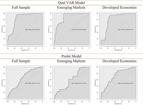
Figure 2. Posterior mean of latent banking crisis indicator with end-of sample forecasts and 68 percent (95 percent where specified) probability interval: Robustness check.

5.3. Variable significance

To analyse economic relationships within vector autoregressive systems, impulse response functions and forecast error variance decompositions (FEVD) are typically applied (Dueker & Assenmacher-Wesche, 2010; Lütkepohl, 1990).

5.3.1. Impulse reponses

Impulse responses describe the dynamic output of a VAR system from an external stimulus. In this study it is based on Cholesky factorization, which renders an efficient computation of complex matrices by decomposing a symmetrically structured positive-finite matrix into a lower triangular matrix. This process introduces orthogonalized shocks to create a moving average representation, where latter innovations depend on previous periods. Based on Lütkepohl (1990), it can be formally stated as follows:

Through a K-dimensional VAR(p), with process $y_t={\mathrm{A}}_1{y}_{\mathit{t}-1}+\dots +$ ${\mathrm{A}}_p{y}_{\mathit{t}-\mathit{p}}+u_t$, given $y_t=(y_{1\mathit{t}},\dots ,y_{\mathit{Kt}}{)}^{\prime }$, A_i the (K x K) coefficient matrices and $u_t=(u_{1\mathit{t}},\dots ,u_{\mathit{Kt}}{)}^{\prime }$, the K-dimensional error term, with $\mathit{E}\left(u_t\right)=0$ and $\mathit{E}\left(u_t,{u^{\prime }}_{\mathit{s}}\right)=\left\{\begin{array}{c}{\mathrm{\Sigma }}_u\mathit{if}\mathit{t}=\mathit{s}\\ 0\mathit{otherwise}\end{array}\right.$with Σ_u positive definite. Assuming covariance stationarity, and orthogonalizing $u_t$, the moving average representation can be denoted as $y_t=\sum _{\mathit{i}=0}^{\mathrm{\infty }}{\varphi }_i{w}_{\mathit{t}-\mathit{i}}$, with ${\varphi }_i={\varphi }_i\mathit{P}$, where triangular matrix P has positive diagonal elements in ${\mathrm{\Sigma }}_u=\mathit{P}{P}^{\prime }$, with $w_t=P^{-1}{u}_t$ so that ${\mathrm{\Sigma }}_w=\mathit{E}\left(w_t{w}_t^{\prime }\right)=I_K$ = (K x K) identity matrix. The responses to initial shocks are ${\psi }_j=\sum _{\mathit{i}=0}^j{\varphi }_i$ and ${\mathrm{\Xi }}_j=\sum _{\mathit{i}=0}^j{\mathrm{\Theta }}_i={\psi }_j\mathit{P}$.

The impulse response is dependent on the ordering of the vector elements, which implies that some variables take longer to respond to shocks, but that causal ordering would not be unique. Yet, Cholesky decomposition remains a straightforward and effective approach to identify shocks within a VAR (Uhlig, 2017).

The recursive variable ordering applied to identify impulse responses is as follows:

{Y*, LRGDP, LCPI, BC, BD, LRER, LRFCF, RIR, BR, TOT, LRPCE, LRE}

where Y* is the latent variable treated endogenously in the VAR. The ordering places gross domestic product, inflation, banking credit and deposits further afront as the subsequent variables are expected to respond within a three-month period once fundamentals weaken.

With a shock applied to the latent variable, average responses for all variables aggregated across all countries are shown in Online Appendix B3 over 12 quarters. With the onset of a banking crisis, gross domestic product instantly declines below zero, and spikes during a subsequent recovery, inflation increases on average by 12 percent before deflation sets in, banking credit and deposit growth remain negative across the forecast horizon and real exchange rates appreciate and depreciate in quick succession over the first six months. Real interest rates decrease below the zero line, reserves weaken gradually, consumption moves into negative territory before improving, with real export growth initially negative while fixed capital formation and terms of trade fluctuate with decreasing magnitude across the 12 quarters. The latent variable is somewhat persistent as crises can last for several periods, becoming smoother between six to ten quarters.

5.3.2. Forecast error variance decomposition

By applying a shock to the VAR system and measuring the resultant change in the forecast error variance, the FEVD reveal the relative importance of each explanatory indicator.

Formally, the proportion of forecast error variance due to innovations in variable j can be described by $w_{\mathit{kj},\mathit{h}}$ where $w_{\mathit{kj},\mathit{h}}=\frac{{\sum }_{i=0}^{h-1}{\theta }_{kj,i}^2}{\mathit{MS}{E}_k\left(\mathit{h}\right)}$ and $w_{\mathit{kj},\mathit{h}}=\frac{{\sum }_{i=0}^{h-1}{({\mathrm{e}}_k^{\prime }{\mathrm{\Theta }}_i{e}_j)}^2}{\mathit{MS}{E}_k\left(\mathit{h}\right)}$ with ${\theta }_{\mathit{kj},\mathit{i}}$ the kj^th element of ${\mathrm{\Theta }}_i$, ${\mathrm{e}}_k$ the k^th column of $I_K$ and the forecast error variance (mean squared error) of h-step ahead forecast of explanatory variable k denoted as $\mathit{MS}{E}_k\left(\mathit{h}\right)=\sum _{\mathit{i}=0}^{\mathit{h}-1}{\mathrm{e}}_k^{\prime }{\varphi }_i{\mathrm{\Sigma }}_u{\varphi }_i^{\prime }{e}_k$.

While forecast error variance decomposition could be sub-optimal due to non-stationary variables (Seyman, 2008), transformations are appropriated for all explanatory indicators as denoted in Table A1 (Appendix A). In interpreting the relations within the system, y* is assumed to be endogenous and the impact of the applied shock examined over 12 quarters.

Results from the forecast error variance decomposition are summarised on an average basis across all countries in Online Appendix B4. Accordingly, real exchange rates constitute a key leading indicator, particularly in the short-term, followed by gross domestic product and banking deposits. Although contributions are dynamic over time, the order generally remains in place with some exceptions. After 12 periods, banking credit has the largest impact followed by real exchange rates and terms of trade.

Findings for all countries are summarized in Online Appendix B5. Some indicators are dominant with above 50 percent contributions such as reserves in the case of Australia, which holds over the immediate period. For Italy, interest rates remain significant across the full period, while banking deposits for Japan and banking credit for Philippines stand out as leading indicators to monitor for ensuing vulnerabilities in the banking sector.

Figure 3 categorizes the results by banking, real and external sector for every country. On average across all countries, banking sector variables contribute approximately 45 percent of total variation, followed by external sector (28 percent) and real sector (21 percent). The relatively higher share of the external sector contains the effects of reduced liquidity due to financial outflows. The balance is captured by y*. For 11 out of 18 countries, the banking sector represents 40 percent or more of the impact. Real sector is particularly important for explaining emerging weaknesses in Finland and Mexico. Activities in the external sector provide a valuable signal for Poland, Spain, Denmark, Sweden, and Thailand.

5.4. Out-of-sample forecast probabilities

Recursive out-of-sample crisis probabilities from the Qual VAR are shown in Table 2. Forecast horizons commence nine to 12-months before the crisis occurred (t-3) and span a total of 12 quarters. Dates for the control group correspond to the juxtaposed crisis countries, highlighting the diversion during the Global Financial Crisis, with time t as onset for the latter cohort. Literature studies highlight a range between 16 percent and 50 percent as threshold levels for predicting economic crises (Birchenhall, Jessen, Osborn, & Simpson, 1999). According to Dueker (2001), the optimal level for minimizing both type 1 and type 2 errors of incorrectly predicting a downturn is 28 percent. Mostly, the escalation and decline in probabilities closely match the subsequent crisis classifications.

Table 2. Out-of-sample forecasts of banking crisis probabilities.

	South Africa 1989		United Kingdom 1991		Colombia 1998-2000		Philippines 1997-2000
Date	Probability	Crisis	Probability	Crisis	Probability	Crisis	Probability	Crisis
t - 3	0.239	0	0.127	0	0.370	0	0.453	0
t - 2	0.338	0	0.230	0	0.697	0	0.718	0
t - 1	0.423	0	0.318	0	0.785	0	0.669	0
t	0.527	1	0.398	1	0.818	1	0.702	1
t + 1	0.576	1	0.455	1	0.833	1	0.685	1
t + 2	0.568	1	0.480	1	0.817	1	0.703	1
t + 3	0.560	1	0.515	1	0.794	1	0.722	1
t + 4	0.564	0	0.540	0	0.766	1	0.717	1
t + 5	0.551	0	0.547	0	0.752	1	0.720	1
t + 6	0.530	0	0.575	0	0.737	1	0.718	1
t + 7	0.517	0	0.586	0	0.710	1	0.721	1
t + 8	0.486	0	0.604	0	0.691	1	0.712	1
	Korea 1997–2000		Costa Rica 1994–1996		France 2008–2014		Spain 2008–2014
Date	Probability	Crisis	Probability	Crisis	Probability	Crisis	Probability	Crisis
t - 3	0.043	0	0.000	0	0.495	0	0.042	0
t - 2	0.050	0	0.242	0	0.702	0	0.188	0
t - 1	0.043	0	0.335	0	0.726	0	0.218	0
t	0.083	1	0.370	1	0.756	1	0.287	1
t + 1	0.142	1	0.392	1	0.800	1	0.302	1
t + 2	0.189	1	0.387	1	0.802	1	0.347	1
t + 3	0.238	1	0.393	1	0.797	1	0.396	1
t + 4	0.278	1	0.397	1	0.814	1	0.418	1
t + 5	0.321	1	0.404	1	0.822	1	0.445	1
t + 6	0.352	1	0.382	1	0.827	1	0.454	1
t + 7	0.385	1	0.380	1	0.823	1	0.458	1
t + 8	0.407	1	0.399	1	0.818	1	0.471	1
	Sweden 2008–2010		Italy 2008–2014		Denmark 2008–2010		Japan control, 2008–2010
Date	Probability	Crisis	Probability	Crisis	Probability	Crisis	Probability	Crisis
t - 3	0.152	0	0.087	0	0.177	0	0.000	0
t - 2	0.432	0	0.393	0	0.197	0	0.113	0
t - 1	0.414	0	0.459	0	0.237	0	0.115	0
t	0.471	1	0.469	1	0.256	1	0.162	0
t + 1	0.404	1	0.443	1	0.273	1	0.165	0
t + 2	0.422	1	0.437	1	0.281	1	0.171	0
t + 3	0.378	1	0.439	1	0.299	1	0.173	0
t + 4	0.383	1	0.445	1	0.309	1	0.191	0
t + 5	0.331	1	0.434	1	0.318	1	0.186	0
t + 6	0.343	1	0.438	1	0.332	1	0.187	0
t + 7	0.302	1	0.435	1	0.354	1	0.184	0
t + 8	0.313	1	0.428	1	0.357	1	0.178	0
	Mexico control, 2008–2010		Thailand control, 2008–2010		Poland control, 2008–2010		Australia control, 2008–2010
Date	Probability	Crisis	Probability	Crisis	Probability	Crisis	Probability	Crisis
t - 3	0.002	0	0.000	0	0.000	0	0.000	0
t - 2	0.077	0	0.000	0	0.117	0	0.000	0
t - 1	0.113	0	0.000	0	0.168	0	0.000	0
t	0.153	0	0.000	0	0.122	0	0.000	0
t + 1	0.160	0	0.000	0	0.142	0	0.000	0
t + 2	0.157	0	0.000	0	0.142	0	0.000	0
t + 3	0.181	0	0.000	0	0.148	0	0.000	0
t + 4	0.189	0	0.000	0	0.134	0	0.000	0
	Mexico control, 2008–2010		Thailand control, 2008–2010		Poland control, 2008–2010		Australia control, 2008–2010
Date	Probability	Crisis	Probability	Crisis	Probability	Crisis	Probability	Crisis
t + 5	0.203	0	0.000	0	0.152	0	0.000	0
t + 6	0.205	0	0.001	0	0.145	0	0.002	0
t + 7	0.218	0	0.002	0	0.153	0	0.006	0
t + 8	0.225	0	0.003	0	0.159	0	0.015	0

During the 1980s-decade, crisis probabilities for South Africa surge from t-3, reaching above 50 percent during the onset of the 1989 banking crisis (t), dipping eight quarters later. The following decade observe probabilities exceeding 80 percent for Colombia, 70 percent in the case of Philippines, 50 percent for United Kingdom and between 30 percent to 40 percent for both Korea Republic and Costa Rica. During the Global Financial Crisis, predictive power for France escalates above 80 percent, whereas Spain, Italy and Sweden exceed 40 percent and Denmark 30 percent, indicative of levels of severity. In contrast, the control group denotes Japan, Mexico and Poland at around 20 percent or lower, with Thailand and Australia on zero.

5.5. Out-of-sample forecast probabilities: robustness check

During a period of the European debt crisis, with t-3 equal to the first quarter of 2013, where several economic fundamentals were under pressure, recursive out-of-sample forecast probabilities for Germany and Finland demonstrate a consistent conclusion, as denoted in Table A4 (Appendix A). In contrast to a burn rate of 300, discarding a larger number of initial iterations delivers a comparable result yet with slightly lower probabilities, which in the case of a tranquil period increases the predictive power. Increasing the number of draws to 2,000 results in marginally higher probabilities for Germany, but lower or similar for Finland, partly due to differences in the frequency distribution of crisis episodes. While the probabilities over a longer forecast horizon exhibit idiosyncratic characteristics, it moves in tandem with the shorter version, denoting its continuation over the last four quarters. Across all forecasts, Finland remains lower than Germany, the latter influenced by its recent experience during the Global Financial Crisis, still lingering in the latent variable.

For policymakers, the Qual VAR approach constitutes a vital instrument as early warning signal. Remaining unaffected by the contagious global banking crises, the control group present valuable evidence on the effectiveness of preventative measures. While a number of studies focus on country-specific experiences during the Global Financial Crisis, sustainable macroeconomic policies and adequately capitalized banks would reinforce banking sector resilience.

5.6. Probit model

To assess the forecasting performance of the Qual VAR, a binary predictor in the form of a probit model constitutes a viable comparison (El-Shagi & Von Schweinitz, 2016). While Qual VAR predicts out-of-sample without knowledge of contemporaneous explanatory values, probit depends on the latter to estimate a probability value. So, although a probit regression does not follow an identical estimation procedure, it remains a useful gauge of imminent frailties.

For the probit model, the identical explanatory variables, log and real transformations are used as with the Qual VAR. For overall comparability, a cross-sectional format is used. Coefficients and statistical significance are shown in Table A5 (Appendix A). Accordingly, the model converges quickly and is statistically significant in comparison to a model without predictors. Predicted probabilities are highly significant for all banking sector variables as well as fixed capital formation in the case of the real sector whereas external sector variables include terms of trade and real exchange rates, corroborating findings by Lindgren, Garcia, and Saal (1996), Hardy and Pazarbasioglu (1998), Demirguc-Kunt and Detregiache (1998).

In-sample regression results render a 60 percent accuracy rate for the combined positive and negative signals. As shown in Table 3, 74 percent of crisis episodes are correctly called, while 54 percent of no-crisis periods are signaled.

Table 3. In-sample probit forecasts.

	Predicted Condition
True Condition		Positive	Negative
	Positive	74%	26%
	Negative	46%	54%

5.7. Results comparison

As based on prediction dates specified in Table A3 (Appendix A), out-of-sample forecast results highlight more accurate crisis predictions for the Qual VAR in comparison to the probit model. Two tests assess predictive performance, with the first encompassing true positive and negative rates and the second using receiver operating characteristics (ROC) with under the curve (AUC) estimations.

The first test institutes a 28 percent threshold level as based on Dueker (2001), centered on an optimal level for minimizing type 1 and type 2 errors, with results shown in Tables 4 and 5. Accordingly, Qual VAR delivers a 93 percent true positive rate against 52 percent for the probit model. While both are sending crisis signals during a tranquil period, true negative rates for the Qual VAR of 75 percent exceeds 66 percent for the probit. In comparison to in-sample performance, overall probit out-of-sample predictive power remains constant on 60 percent, where true positive rates eminently reduce, however including explanatory information, results in more true negative signals.

Table 4. Out-of-sample Qual VAR forecasts.

	Predicted Condition
True Condition		Positive	Negative
	Positive	93%	7%
	Negative	25%	75%

Table 5. Out-of-sample probit forecasts.

	Predicted Condition
True Condition		Positive	Negative
	Positive	52%	48%
	Negative	34%	66%

The second test, which revolves around AUROC (area under receiver operating characteristic curve) estimates, feature in business cycle studies including Berge and Jord`a (2017) and Döpke, Fritsche, and Pierdzioch (2017), and plot true and false positive rates at different cut-off points. Results denoted in Table 6 show Qual VAR outperforming the probit model with a mean of 85 percent to 66 percent. Disaggregating Qual VAR prediction output according to emerging markets and developed economies demonstrates comparable results, although a slightly stronger predictive power notable for the former. The ROC curves are plotted in Figure 4. A salient benefit of the ROC curves involves the availability of different levels of sensitivity and specificity, from which an appropriately selected probability of a banking crisis indicates a concomitant policy response.

Table 6. Out-of-sample forecasts: AUROC results.

	Qual VAR			Binomial
	Full Sample	Emerging Markets	Developed Economies	Probit Model
Mean	0.850	0.887	0.827	0.666
CI Lower Bound	0.797	0.813	0.746	0.591
CI Upper Bound	0.904	0.962	0.907	0.741
Standard Error	0.027	0.038	0.041	0.038

Upper and lower bounds are based on 95 percent confidence intervals. Variance of AUC is defined by DeLong, DeLong, and Clarke-Pearson (1988) and estimated with algorithm specified by Sun and Weichao (2014).

6. Concluding remarks

In support of remedial efforts by policymakers, the paper examines 40 years of banking crises, encompassing a final sample of 18 countries, which experienced a combined 34 crises. Extending on the traditional vector autoregression system, the Qual VAR methodology accommodates qualitative information on banking sector crises through a binary choice variable and conflated with macroeconomic information produces a continuous banking crisis indicator. In fusing with the 12 variable VAR, a latent variable y* is based on banking crisis classifications and utilized to determine crisis probabilities. Centered on empirical literature, the study draws on leading explanatory indicators, including gross domestic product, investment, consumption, inflation, interest rates, banking assets and liabilities, exchange rates, terms of trade, reserves, and exports. During the period under review, precursors to banking crises have dynamically evolved. In this regard, a representative sample of countries form part of the study in order to capture the effects across period, region, and level of development. Forecast error variance decomposition highlights the importance of banking sector variables, in addition to external and real sectors. Moreover, country-level monitoring remains paramount.

Findings on predictive power suggest that recursive out-of-sample forecasts up to 12-months preceding a banking crisis render distinctive and reliable results for most countries, and through a continuous latent variable argue a compelling case for unremittent monitoring and evaluation of precursors to banking sector frailties. Notwithstanding the limitations on observations of banking crises, for the final 18 countries under review, the posterior mean of the latent variable converges to or crosses zero for most out-of-sample forecasts, while the counterfactual selection emphasizes a diverging trend towards unity. Predictive probabilities are dynamically estimated and exceed a 28 percent threshold in all instances, reaching above 80 percent in certain cases, whereas non-crisis control group countries all register below the threshold, with some denoting zero. In comparison to a probit model, Qual VAR outperforms out-of-sample with higher true positive and true negative rates and as based on area under curve receiver operating characteristics.

Incorporating microeconomic and bank-level data and findings from non-crisis countries constitute future research areas. With banking crises manifesting as a periodic phenomenon impacting developed economies and emerging markets with severe repercussions to the socioeconomic and political environment, the Qual VAR makes a valuable contribution to the examination and prognostication of modulation between crisis and tranquil periods. In turn, policymakers, central banks, and banking oversight departments become better equipped to formulate alleviating measures, in advance.

Acknowledgments

I am grateful to the editor, an anonymous referee, Ulrich Fritsche for his guidance, Olivier Damette and conference participants at the 2019 Augustin Cournot Doctoral Days at the University of Strasbourg in France for valuable suggestions and comments.

Disclosure statement

No potential conflict of interest was reported by the author.

Supplementary material

Supplemental data for this article can be accessed here.

Additional information

Notes on contributors

Emile du Plessis

Emile du Plessis is a senior economist at Standard Bank. His forecasts on international capital and money markets, equities, commodity prices, currencies, reserves, credit, inflation, national budget and domestic production are published weekly by Bloomberg and Reuters. He received the 2019 Refinitiv StarMine Award for Most Accurate Forecasting in a Reuters poll. Emile served on the Academic Management Board of the Bureau of Market Research at UNISA. He received his Bachelor of Arts degree in Political, Philosophical and Economic Studies, Bachelor of Commerce with Honors degree in Economics and Master of Commerce degree in Economics from the University of Stellenbosch in South Africa and is completing his PhD in Economics at the University of Hamburg in Germany. His research interests include banking crises, systemic financial risks, early warning indicators, econometric modelling, forecasting and machine learning and behavioural and experimental economics. He established and leads an applied Behavioural Economics capability across 15 African countries. It includes a unique mastery programme focused on future skills development that equips staff to operate in the fourth industrial revolution.

Appendix A

Table A1. Variables and transformations.

Variable	Definition	Category	Source
LRGDP	Annualized real gross domestic product growth, in logs	Real	IFS
LRPCE	Annualized real consumption expenditure growth, in logs	Real	IFS
LRFCF	Annualized real fixed capital formation growth, in logs	Real	IFS
BD	Ratio of bank deposits relative to gross domestic product	Banking	IFS
BC	Ratio of bank credit to private sector to gross domestic product	Banking	IFS
BR	Reserves as ratio to gross domestic product	Banking	IFS
LCPI	Annualized consumer inflation growth, in logs	Banking	IFS
RIR	Real interest rates	Banking	IFS
LRER	Annualized real exchange rate growth, in logs	External	IFS
TOT	Imports to exports as proxy for terms of trade	External	IFS
LRE	Annualized real exports growth, in logs	External	IFS

Table A2. Unit-root tests.

ADF – Fisher Test (Levels)
Variable	Specification	Inverse chi-squared	Inverse normal	Inverse logit t	Modified inv. chi-squared
LRDGP	c,4	91.655***	−5.606***	−5.924***	7.456***
LRPCE	c,4	176.912***	−9.811***	−12.146***	18.114***
LRFCF	c,4	130.472***	−7.895***	−8.849***	12.309***
BD	c,4	24.184	1.623	1.511	−0.976
BC	c,4	23.066	3.212	3.742	−1.116
BR	c,4	62.092***	−1.634**	−2.212**	3.761***
LCPI	c,4	64.881***	−3.750***	−3.790***	4.110***
RIR	c,4	42.918*	−1.745**	−1.684**	1.364*
LRER	c,4	191.417***	−10.186***	−13.111***	19.927***
TOT	c,4	46.622**	−1.439*	−1.306*	1.827**
LRE	c,4	188.645***	−10.605***	−13.024***	19.580***
Phillips-Perron – Fischer Test (Levels)
LRDGP	c,4	984.373***	−29.573***	−68.251***	119.046***
LRPCE	c,4	1046.933***	−30.706***	−72.589***	126.866***
LRFCF	c,4	787.818***	−25.543***	−54.623***	94.477***
BD	c,4	25.729	1.790	1.640	−0.783
BC	c,4	85.513***	0.313	−2.104**	6.689***
BR	c,4	42.572*	−0.592	−0.574	1.321*
LCPI	c,4	498.250***	−19.005***	−34.536***	58.281***
RIR	c,4	62.686***	−3.687***	−3.591***	3.835***
LRER	c,4	676.290***	−23.315***	−46.867***	80.536***
TOT	c,4	152.946***	−7.071***	−9.457***	15.118***
LRE	c,4	1041.946***	−30.667***	−72.243***	126.243***

Unit root tests are constructed using Augmented Dicky-Fuller (see Hamilton, 1994) and Phillips and Perron (see Phillips & Perron, 1988) procedures. Based on Choi (2001), four different methods are assessed to test the null hypothesis of a unit root across all panels, through an inverse, inverse-normal, inverse-logit transformation and a modification of the inverse transformation of the p-values. The latter is appropriate for N → ∞.

Table A3. Out-of-sample prediction dates.

IFS Code	Country	Crisis	No-Crisis
112	United Kingdom	2007–2014
128	Denmark	2008–2014
132	France	2008–2014
134	Germany		2013–2016
136	Italy	2008–2014
144	Sweden	2008–2010
158	Japan		2008–2014
172	Finland		2013–2016
184	Spain	2008–2014
193	Australia		2008–2014
199	South Africa	1989
233	Colombia	1998–2000
238	Costa Rica	1994–1996
273	Mexico		2008–2014
542	Korea Republic	1997–2000
566	Philippines	1997–2001
578	Thailand		2008–2014
964	Poland		2008–2014

A selection of countries that did not experience banking distress during the Global Financial Crisis (GFC) serve as control group for out-of-sample testing. In the case of Germany and Finland, a more recent period is selected to test applicability of out-of-sample predictive power, particularly during the European sovereign debt crisis.

Table A4. Out-of-sample forecasts of banking crisis probabilities: robustness check.

Germany, control, 2013–2015
	Burn 300; Draw 1,200	Burn 1,000; Draw 1,200	Burn 300; Draw 2,000	Burn 1,000; Draw 2,000
Date	Probability				Crisis
t - 3	0.000	0.000	0.053	0.000	0
t - 2	0.013	0.005	0.092	0.038	0
t - 1	0.072	0.013	0.140	0.070	0
t	0.097	0.040	0.180	0.146	0
t + 1	0.134	0.054	0.207	0.145	0
t + 2	0.148	0.086	0.235	0.203	0
t + 3	0.196	0.116	0.251	0.209	0
t + 4	0.219	0.141	0.295	0.249	0
t + 5	0.263	0.165	0.305	0.240	0
t + 6	0.256	0.189	0.337	0.281	0
t + 7	0.282	0.213	0.350	0.272	0
t + 8	0.285	0.214	0.353	0.311	0
Finland, control, 2013–2015
	Burn 300 Draw 1,200	Burn 1,000; Draw 1,200	Burn 300; Draw 2,000	Burn 1,000; Draw 2,000
Date	Probability				Crisis
t - 3	0.029	0.000	0.011	0.012	0
t - 2	0.048	0.003	0.020	0.021	0
t - 1	0.122	0.009	0.040	0.066	0
t	0.116	0.013	0.051	0.071	0
t + 1	0.142	0.021	0.069	0.098	0
t + 2	0.133	0.026	0.073	0.105	0
t + 3	0.144	0.027	0.075	0.122	0
t + 4	0.147	0.030	0.075	0.128	0
t + 5	0.150	0.032	0.086	0.137	0
t + 6	0.159	0.043	0.092	0.140	0
t + 7	0.157	0.048	0.102	0.149	0
t + 8	0.144	0.052	0.100	0.148	0
	Germany, control, 2013–2016			Finland, control, 2013–2016
Date	Probability		Crisis
t - 3	0.000		0	0.053
t - 2	0.031		0	0.060
t - 1	0.053		0	0.075
t	0.119		0	0.086
t + 1	0.128		0	0.105
t + 2	0.171		0	0.108
t + 3	0.172		0	0.122
t + 4	0.217		0	0.126
t + 5	0.237		0	0.130
t + 6	0.268		0	0.139
t + 7	0.277		0	0.154
t + 8	0.279		0	0.159
t + 9	0.290		0	0.000
t + 10	0.282		0	0.000
t + 11	0.260		0	0.000
t + 12	0.259		0	0.000

Table A5. Probit model results.

Probit Results
No. of observations:	1,200
Constrained log-likelihood:	−732.187
Max. log-likelihood:	−653.420
LR-chiˆ2:	157.53***
AIC:	1.109
BIC:	−7116.170
Variable	dy/dx
LRDGP	0.440 (0.745)
LRPCE	0.175 (0.560)
LRFCF	−0.761 (0.389)***
BD	0.462 (0.071)***
BC	−0.335 (0.048)***
BR	−0.016 (0.003)***
LCPI	6.801 (2.040)***
RIR	0.027 (0.006)***
LRER	−3.636 (0.309)***
TOT	0.000 (0.000)***
LRE	−0.363 (1.072)

Margins with standard errors in brackets, *** 1% level of significance

References

- Abiad, A. (2003). Early-warning systems: A survey and a regime-switching approach. IMF Working Paper, WP/03/32.
- Albert, J. H., & Chib, S. (1993). Bayesian analysis of binary and polychotomous response data. Journal of the American Statistical Association, 88(422), 669–679.
- Alessi, L., & Detken, C. (2011). Quasi real time early warning indicators for costly asset price boom/bust cycles: A role for global liquidity. European Journal of Political Economy, 27(3), 520–533.
- Barrell, R., Davis, E., Karim, D., & Liadze, I. (2010). Bank regulation, property prices and early warning systems for banking crises in OECD countries. Journal of Banking and Finance, 34(9), 2255–2264.
- Berg, A., Borensztein, E., & Pattillo, Z. (2005). Assessing early warning systems: How have they worked in practice? IMF Staff Papers, 52, 3.
- Berge, T. J., & Jord`a, O. (2011). Evaluating the classification of economic activity into recessions and expansions. American Economic Journal, Macroeconomics, 3(2), 246–277.
- Birchenhall, C. R., Jessen, H., Osborn, D. R., & Simpson, P. W. (1999). Predicting U.S. business cycle regimes. Journal of Business and Economic Statistics, 17(3), 313–323.
- Bordo, M., Dueker, M. J., & Wheelock, D. (2008). Inflation, monetary policy and stock market conditions. NBER Working Paper, 14019, National Bureau of Economic Research.
- Bordo, M., Eichengreen, B., Klingebiel, D., & Martinez-Peria, M. S. (2001). Is the crisis problem growing more severe? Economic Policy, 16, 51–82.
- Bussière, M., & Fratzscher, M. (2006). Towards a new early warning system of financial crises. Journal of International Money and Finance, 25(6), 953–973.
- Calomiris, C. (2010). The great depression and other ‘contagious’ events. The Oxford Handbook of Banking. Oxford: Oxford University Press.
- Caprio, G., & Klingebiel, D. (1996). Bank insolvencies: Cross-country experience. Working Paper, Number 1620. World Bank.
- Caprio, G., & Klingebiel, D. (2003). Episodes of systemic and borderline financial crises. In Managing the Real and Fiscal Effects of Banking Crises edited by Klingebiel, D and Laeven, L., World Bank Discussion Paper 428, 31-49. Washington, D.C.: World Bank.
- Chauvet, M. (1998). An econometric characterization of business cycle dynamics with factor structure and regime switching. International Economic Review, 39(4), 969–996.
- Chauvet, M., & Potter, S. (2003). Predicting recessions using the yield curve. Journal of Forecasting, 24(2), 77–103.
- Chauvet, M., & Potter, S. (2010). Business cycle monitoring with structural changes. International Journal of Forecasting, 26(4), 777–793.
- Chib, S. (1993). Bayes regression with autoregressive errors: A Gibbs sampling approach. Journal of Econometrics, 58(3), 275–294.
- Choi, I. (2001). Unit root tests for panel data. Journal of International Money and Finance, 20(2), 249–272.
- Claessens, S., Kose, M. A., & Terrones, M. (2011). The global financial crisis: How similar? How different? How costly? Journal of Asian Economics, 21(3), 247–264.
- DeLong, E. R., DeLong, D. M., & Clarke-Pearson, D. L. (1988). Comparing the areas under two or more correlated receiver operating characteristic curves: A nonparametric approach. Biometrics, 44(3), 837–845.
- Demirgüç-Kunt, A., & Detragiache, E. (2000). Monitoring banking sector fragility: A multivariate logit approach. The World Bank Economic Review, 14(2), 287–307.
- Demirguc-Kunt, A., & Detregiache, E. (1998). The determinants of banking crises in developing and developed countries. IMF Staff Papers, 45(1). Washington: International Monetary Fund.
- Döpke, J., Fritsche, U. and Pierdzioch, C. 2017. “Predicting Recessions with Boosted Regression Trees. International Journal of Forecasting, Vol 33, pp 745–759.
- Dueker, M. J. (1999). Conditional heteroscedasticity in qualitative response models of time series: A Gibbs sampling approach to the bank prime rate. Journal of Business and Economic Statistics, 17(4), 466–472.
- Dueker, M. J. (2001). Forecasting qualitative variables with vector autoregressions: A Qual VAR model of U.S. recessions, Federal Reserve Bank of St. Louis, Working Paper 012A.
- Dueker, M. J. (2003). Dynamic forecasts of qualitative variables: A Qual VAR model of U.S. recessions. Federal Reserve Bank of St. Louis, Working Paper, 2001-012B. Revised 2003.
- Dueker, M. J. (2005). Dynamic forecasts of qualitative variables. Journal of Business and Economic Statistics, 23, 96-104.
- Dueker, M. J., & Assenmacher-Wesche, K. (2010). Forecasting macro variables with a Qual VAR business cycle turning point index. Applied Economics, 42(23), 2909-2920.
- Eichenbaum, M., & Evans, C. L. (1995). Some empirical evidence on the effects of shocks to monetary policy on exchange rates. Quarterly Journal of Economics, 110(4), 975–1009.
- Eichengreen, B. J., Watson, M. W., & Grossman, R. S. (1985). Bank rate policy under the interwar gold standard: A dynamic probit model. The Economic Journal, 95(379), 725–745.
- El-Shagi, M., & Von Schweinitz, G. (2016). Qual VAR revisited: Good forecast, bad story. Journal of Applied Economics, 19(2), 293–321.
- Filardo, A. J. (1994). Business cycle phases and their transitional dynamics. Journal of Business and Economic Statistics, 12(3), 299–308.
- Fornari, F., & Lemke, W. (2010). Predicting recession probabilities with financial variables over multiple horizons. European Central Bank, Working Paper Series, 1255.
- Frankel, J., & Saravelos, G. (2012). Can leading indicators assess country vulnerability? Evidence from the 2008–09 global financial crisis. Journal of International Economics, 87(2), 216–231.
- Frankel, J. A., & Rose, A. K. (1996). Currency crashes in emerging markets: An empirical treatment. Journal of International Economics, 41(3), 351-366.
- Fratzscher, M. (2003). On currency crises and contagion. International Journal of Finance and Economics, 8(2), 109–129.
- Galvão, A. (2006). Structural break threshold VARs for predicting US recessions using the spread. Journal of Applied Econometrics, 21(4), 463–487.
- Goldfeld, S. M., & Quandt, R. E. (1973). A Markov model for switching regressions. Journal of Econometrics, 1(1), 3–16.
- González-Hermosillo, B., Pazarbasioglu, C., & Billings, R. (1997). Determinants of banking sector fragility: A case study of Mexico. IMF Staff Papers, 44(3). Washington: International Monetary Fund.
- Gupta, R., & Wohar, M. E. (2015). Forecasting oil and stock returns with a Qual VAR using over 150 years of data. University of Pretoria, Working Paper, 2015-89.
- Hamilton, J. (1989). A new approach to the economic analysis of nonstationary time series and the business cycle. Econometrica, 57(2), 357–384.
- Hamilton, J. D. (1990). Analysis of time series subject to changes in regime. Journal of Econometrics, 45(1–2), 39–70.
- Hamilton, J. D. (1994). Time Series Analysis. Princeton: Princeton University Press.
- Harding, D., & Pagan, A. (2011). An econometric analysis of some models for constructed binary time series. Journal of Business and Economic Statistics, 29(1), 86–95.
- Hardy, D. C., & Pazarbasioglu, C. (1998). Leading indicators of banking crises: Was Asia different? IMF Working Paper, WP/98/91.
- Hartmann, P., Hubrich, K., Kremer, M., & Tetlow, R. (2015). Melting Down: Systemic Financial Instability and the Macroeconomy.SSRN. Available at http://dx.doi.org/10.2139/ssrn.2462567.
- IMF. (1998). Financial crises: Causes and indicators, world economic outlook. Washington D.C: International Monetary Fund.
- IMF. (2018). International financial statistics. Yearbook 2018. Washington D.C: International Monetary Fund.
- Kaminsky, G., Lizondo, S., & Reinhart, C. M. (1998). Leading indicators of currency crises. Staff Papers - International Monetary Fund, 45(1), 1.
- Kaminsky, G., & Reinhart, C. (1999). The Twin Crises: The Causes of Banking and Balance-of-Payments Problems. American Economic Review, 89(3), 473–500.
- Kauppi, H., & Saikkonen, P. (2008). Predicting U.S. recessions with dynamic binary response models. The Review of Economics and Statistics, 90(4), 777–791.
- Kim, C.-J., & Nelson, C. R. (1998). Business cycle turning points, a new coincident index, and tests of duration dependence based on a dynamic factor model with regime switching. Review of Economics and Statistics, 80(2), 188–201.
- Knedlik, T., & Von Schweinitz, G. (2012). Macroeconomic imbalances as indicators for debt crises in Europe. JCMS: Journal of Common Market Studies, 50(5), 726–745.
- Laeven, L., & Valencia, F. (2010). Resolution of banking crises: The good, the bad and the ugly. IMF Working Paper, Number 10/146.
- Laeven, L. and Valencia, F. (2018). Systemic banking crises revisited. IMF Working Paper, WP/18/206.
- Lindgren, C. J., Garcia, G., & Saal, M. I. (1996). Bank soundness and macroeconomic policy. Washington: IMF.
- Lütkepohl, H. (1990). Asymptotic distributions of impulse response functions and forecast error variance decompositions of vector autoregressive models. The Review of Economics and Statistics, 72(1), 116–125.
- Meinusch, A., & Tillmann, P. (2015). The macroeconomic impact of unconventional monetary policy shocks. Journal of Macroeconomics, 47(PA), 58-67.
- Nyberg, H. (2010). Dynamic probit models and financial variables in recession forecasting. Journal of Forecasting, 29(1–2), 215–230.
- Paap, R., Segers, R., & Van Dijk, D. (2009). Do leading indicators lead peaks more than troughs? Journal of Business and Economic Statistics, 27(4), 528–543.
- Phillips, C. B., & Perron, P. (1988). Testing for a unit root in time series regression. Biometrika, 75(2), 335–346.
- Quandt, R. E. (1958). The Estimation of the Parameters of a Linear Regression System Obeying Two Separate Regimes. Journal of the American Statistical Association, 53(284), 873–880.
- Reinhart, C. M. (2002). Default, currency crises, and sovereign credit ratings. The World Bank Economic Review, 16(2), 151–170.
- Reinhart, C. M., & Rogoff, K. S. (2009). This time is different: Eight centuries of financial folly. New Jersey: Princeton University Press.
- Rudebusch, G., & Williams, J. (2009). Forecasting recessions: The puzzle of the enduring power of the yield curve. Journal of Business and Economic Statistics, 27(4), 492–503.
- Seyman, A. (2008). A critical note on the forecast error variance decomposition. Centre for European Economic Research, Discussion Paper, 08-065.
- Shin, I., & Hahm, J. H. (1998). The Korean crisis: Causes and resolution. Korea Development Institute Working Paper.
- Sims, C. A. (1980). Macroeconomics and reality. Econometrica, 48(1), 1–48.
- Stock, J. H., & Watson, M. W. (2001). Vector Autoregressions. Massachusetts: National Bureau of Economic Research.
- Sun, X., & Weichao, X. (2014). Fast implementation of Delongs algorithm for comparing the areas under correlated receiver operating characteristic curves. IEEE Signal Processing Letters, 21(11), 1389–1393.
- Uhlig, H. (2017). Shocks, sign restrictions and identification. In B. Honoré, M. Pakes, M. Piazzesi, & L. Samuelson (Eds.), Advances in economics and econometrics: Eleventh world congress, econometric society monographs. Cambridge: Cambridge University Press, 95-127.
- Vlaar, P. J. G. (1999). Currency crises models for emerging markets. Research Memorandum WO&E 595/9928, 1-32.