Money and inflation in inflation-targeting regimes – new evidence from time–frequency analysis

ABSTRACT

This article investigates the post-1990 link between broad money growth and inflation in 16 full-fledged inflation-targeting regimes and four benchmark non-inflation-targeting regimes. This study employs the Christiano-Fitzgerald band-pass filter and continuous wavelet transform to analyze the co-movements across operational horizons and time. According to the band-pass filtering techniques, the link between money growth and inflation was weak and statistically nonsignificant over the investigated period: from 1990 onwards. The wavelet analysis demonstrated significant causality running from money growth to inflation, and strong significant co-movements between the two variables around the Great Recession at a typical business cycle frequency. This finding suggests that policymakers may need to respond to the short-run surges in money growth by reducing money growth rates. The empirical findings support the proposal that policymakers should return to a monetary framework that controls the money supply.

KEYWORDS:

• Money and inflation
• inflation targeting
• quantity theory of money
• money demand
• wavelets

1. Introduction

The one-for-one long-run association of money growth and inflation is confirmed by data from different countries, centuries, and monetary policy regimes. Since 1990, this famous relationship seems to have disappeared from simple scatterplots in low-inflation countries (Teles, Uhlig, & Azevedo, 2016). The relevance of the disappearance for the alleged breakdown of quantity theory is high. Simple and long-run correlations (or sometimes the lead-lag relationships) constituted a primary method through which the theory was advocated. Simple correlations have even been argued to deliver more-certain knowledge than structural models because of their independence from the sometimes-questionable assumptions of more-advanced methods.

The goal of this article is to assess how far broad money growth‡ and consumer inflation have moved away from the quantity theory in countries that adopted full-fledged inflation targeting¹ (FFIT) since 1990 and account for the period after the 2007 global financial crisis. The existence, stability, and causation of a relation between money and inflation are relevant to inflation targeting (IT) regimes, including the implications for policy. Assuming that a stable money‐demand function exists, the relation could be helpful to forecast the behaviour of output and inflation in the longer run, in line with classical monetary theory.

The role of money (Sławiński, 2019; Temizsoy & Montes-Rojas, 2019) and global liquidity (Avdjiev et al., 2018) in the conduct and design of monetary policy have re-emerged as a relevant issue since the 2007 global financial crisis. The renewed interest in money stems from rising money and credit arrangements and the undisputed role played by the financial sector in the propagation and origination of the Great Recession. The importance of money and global liquidity has increased recently even more because of the COVID-19 pandemic and the related further easing of monetary conditions by many central banks. In particular, the Fed and the Bank of Japan – both inflation targeters since 2012 and 2013, respectively – announced unlimited asset purchases in response to the economic slowdown due to the coronavirus crisis. Asset purchases predominantly from non-bank financial companies are intended to increase the amount of money available and stimulate spending (McLeay, Radia, & Thomas, 2014).

The unprecedented scale of these purchases has encouraged practitioners and academia to study their macroeconomic impact (Hohberger, Priftis, & Vogel, 2019; Matousek, Papadamou, Šević, & Tzeremes, 2019). The financial system, filled with abundant liquidity and characterized by fundamental changes of money and credit (Ryczkowski, 2020; Schularick & Taylor, 2012), caused others to deliberate on the possible unintended medium- and longer-run consequences of such an “ultra-easy” monetary policy (Ciżkowicz & Rzońca, 2017). In particular, the accommodative monetary policy created concerns about its inflationary risks (Giraud & Pottier, 2016; van den End, 2016). Notably, Taylor (2019), and Belongia and Ireland (2018) argue for targeting the growth rate of monetary aggregates in the post-crisis environment. However, the existence of a long‐run money and inflation link is important for a rule‐based monetary policy with importance assigned to money.

The new relevance assigned to money and credit in macroprudential policy and trials to adjust cashless and dynamic stochastic general equilibrium (DSGE) models with financial frictions might be opposed to the conception of pre-crisis IT. Pre-crisis IT typically relies on the downgraded role of money and the primary importance assigned to the Taylor-type rules and interest rates (Ryczkowski, 2017). The aforementioned discrepancy constitutes a natural background to analyze the association between money growth and inflation in inflation-targeting regimes.

The contribution of this article is to fill a gap in the literature on the link between money and inflation in inflation-targeting regimes in general and especially in the post-Great Recession era. The cross-country evidence concerns predominantly the pre-crisis environment (see, Grauwe & Polan, 2014; Teles et al., 2016). However, even if the post-crisis results are available, they concern typically single major economies (see, Christev & Kang, 2015; Ellington & Milas, 2019; Hossain, 2019b). Consequently, there is a gap in the literature for at least some of the FFIT countries. Moreover, the available post-crisis results are often not compared to the analogous findings for other inflation targeters and leading non-inflation targeters. The notable two exceptions are the articles of Breuer, Mcdermott, and Weber (2018) and Gertler and Hofmann (2018), which include the period until 2010 for 99 countries and until 2011 for 46 countries, respectively. However, the authors have constructed panels that do not include solely IT, limiting the possibility to draw IT-specific and country-specific conclusions.

In the literature, the confusion over the significance of the relationship between money growth and inflation stems from the deterioration of the relationship in low-inflation environments, on the one hand (Sargent & Surico, 2011), and the evidence that has presented a strong link between money and inflation, on the other hand (Cooray & Khraief, 2019; Fedotenkov, 2018).

Studies on the long-run (low-frequency) developments between money growth and inflation are of several types. An argument is that the long-run average changes in the quantity of money create an equal change of price inflation for cross-sections of countries (Gertler & Hofmann, 2018) – at least when high-inflation countries are in the sample. Band-pass filters are broadly used to extract low-frequency cycles. Haug and Dewald (2011) find that the long-run correlations are almost all positive, high, significant, and stable over time for the 11 countries from 1880 to 2001. Similarly, wavelet transform can capture the frequency-varying features, but without predefining the constant frequency band. Despite this feature, wavelet transform is a rarely used method to study the link between money growth and inflation. For instance, Jiang, Chang, and Li (2015) argue from the wavelet perspective that money growth and inflation are related to in a one-to-one fashion in the medium and long runs in China.

Finally, applying cointegration to find a stationary linear combination between money growth, inflation, and other non-stationary time series usually supports monetarist theory (Hossain, 2019a). Studies that rely on structural estimation are less frequently published. An example of these studies is Cooray and Khraief (2018). They apply a nonlinear auto‐regressive distributed lag model over a long-run time span and find that money growth and inflation are significantly linked in the post‐crisis period in the United Kingdom but not to that in the United States and Japan. Morana (2006) estimates a small-scale macroeconometric model for the euro area and applies co-breaking and fractional cointegration theory to justify the two-pillar monetary policy of the European Central Bank.

The remainder of this article is organized as follows. Section 2 reviews the contemporary evidence on the relationship between money and inflation in a modern, globalized, and low-inflation environment and presents the plausible reasons for the deterioration of the relationship. Section 3 describes the data. Section 4 presents the methodology. The empirical results are discussed in Section 5. Causality across time and frequency is assessed with the wavelet phase difference and compared to the Granger causality. Co-movements across time and frequency are analyzed with the continuous wavelet transform and the Christiano-Fitzgerald band-pass filter. The robustness checks are based on, for example, maximal overlap discrete wavelet transform.

2. Literature review

The reasons for the deterioration of the relationship between money growth and inflation can be divided into four groups: new monetary policy regimes, changes in the velocity of money, globalization, and other factors.

Sargent and Surico (2011) explain the alleged breakdown of quantity theory on the basis of the new monetary policy regimes, which respond aggressively to inflationary pressure. Modern central banks ensure that the process of money creation is consistent with the inflation target, and the quantity of loans and deposits in the economy is mostly created by commercial banks (McLeay et al., 2014). Fisherian movements in interest rates and a decrease in the opportunity cost of money changed the money demand and distorted the assumption of the linear trend-stationary velocity of money (Teles et al., 2016).

In summary, new institutions and the behaviour of macroeconomic variables affect the income velocity of money (Nunes, St. Aubyn, Valério, & de Sousa, 2018). If velocity is unstable (Grauwe & Polan, 2014), the money per unit of income is also unstable. Berentsen, Huber, and Marchesiani (2015) argue that the improved access to money markets explains the new money demand. Individuals changed how they hold assets, because of deregulation (Fanta, 2013), financial innovations, common access to ATM cards, increasing role of money substitutes (Berentsen et al., 2015), new production technology and the preference structure (Itaya & Mino, 2007), changes in operational management, and financial intermediation increasing in complexity (Long, Goswami, & Jobst, 2009). Technological progress in financial technologies allowed banks and households to increase their financial leverage even during monetary tightening. New electronic money and digital currencies might also change the demand for money. Despite this phenomenon, studies have accounted for variables, for example, foreign risky assets (De Santis, 2015), to obtain the stability of money demand in line with quantity theory.

Borio and Filardo (2007) regard increasing openness of the international economy (Zhang, 2017) as a complementary explanation to a more effective monetary policy in explaining the currently satisfactory inflation performance. Cheap imports from emerging markets (Boehlke, Faldzinski, Galecki, & Osinska, 2020; Bugamelli, Fabiani, & Sette, 2015), an inflow of lower-cost labour, and the growth of productivity because of the inclusion of computer-based information technology in productive processes (Edquist & Henrekson, 2017), the rising quality of inputs (Vandenberghe, 2017), improved cyclical conditions (Buiter, 2000), or simply good luck (Stock & Watson, 2007) decrease overall price inflation. In turn, higher demand resulting from the integration of emerging countries into the global economy may drive up prices for energy and raw materials and eventually increase prices of general commodities. The two-way influence of globalization on prices might explain the globalization–inflation “puzzle” (Temple, 2002) and can impede the extraction of the stable link between money growth and inflation. Moreover, in a globalized world, cross-border capital inflows and outflows might affect domestic credit beyond the volume that would result from domestic monetary conditions (Liu & Kool, 2018).

The continuing controversy over the money growth–inflation relationship is linked to the problems with the “right” definition of money and the technical difficulty of sorting out the direction of causation between money and prices. Quantity theory might also be violated because of the limitations of monetary policy. In a liquidity trap, the quantity of money is irrelevant because money and bonds become perfect substitutes, for instance, Bacchetta, Benhima, and Kalantzis (2019) argue that quantitative easing leads to a deepening of a liquidity trap. Additionally, when the CPI index is used to analyze the quantity theory, the representativity of the market basket and the well-known limitations of the index determine the accuracy of measuring inflation. Finally, ideological concerns over the viability of market mechanisms allow the discussion to prevail.

Despite the aforementioned reasons for the deterioration of the link between money growth and inflation, some researchers have warned that the link can reoccur. Roffia and Zaghini (2007) present evidence that the probability of an inflationary outburst increases, especially when money growth is accompanied by loose credit conditions and increases in stock and house prices. An increase in inflation or money growth would restore the strong link between money growth and inflation (Ellington & Milas, 2019; Gertler & Hofmann, 2018; Sargent & Surico, 2011). Therefore, monitoring monetary conditions and the monetary policy stance seem to be especially important during quantitative easing and when policy rates move toward their zero lower bound (Belongia & Ireland, 2018). However, the issue is inconclusive. Kočenda and Varga (2018) claim that flexible IT is optimal during and after the financial crisis. Other economists have opted for an even larger weight on economic activity than on inflation in central banks’ loss functions, to more rapidly return post-crisis underemployment to normal levels (Debortoli, Kim, Lindé, & Nunes, 2019).

3. Data

The quarterly data range from 1Q 1990 to 1Q 2017. The starting date corresponds to an effective adoption of the first inflation-targeting strategy in New Zealand. Data for consumer inflation for all items, for the real and nominal gross domestic product (GDP), and for the private final consumption expenditure of households and non-profit institutions serving households are from the Organisation for Economic Co-operation and Development (OECD). Data for the monetary aggregate M3 are predominantly from the International Financial Statistics database of the International Monetary Fund (IMF) [US, CA, JP, SE, ZA, CL, MX, PL] and from the Federal Reserve Bank of St. Louis (AU, NZ, NO, DK, CH, EA, HU, IL, CZ). For South Korea and Iceland, I use the IMF broad money (M2) time series and the OECD broad money index, respectively. In the United States, data for M3 are available until 4Q 2005. The Fed ceased their publication that was once found on the official website because M3 “does not appear to convey any additional information on economic activity that is not already embodied in M2 […].” Since 2006, M3 data were extrapolated with the growth rate of a broad money index from the Monthly Monetary and Financial Statistics of OECD. For the United Kingdom, I use the break adjusted broad money time series from the Bank of England. All the time series are seasonally adjusted. More data details are given in the notes corresponding to the presented figures.

Denmark, the United States, Japan, and the euro area comprise the group of benchmark low-inflation, non-inflation targeters. Although Denmark’s monetary policy aims to maintain the stability of the krone against the euro within the fixed-exchange-rate policy, the three remaining economies adopted inflation targets; however, these economies are not considered full-fledged inflation-targeting regimes.²

4. Methodology

The exercises are performed for all the regimes considered from 1Q 1990 to 1Q 2017, unless stated otherwise, despite the difference in the adoption dates of the full-fledged inflation targeting (Table 1). The first reason for using this method is that it increases the comparability between the 16 FFIT and especially between the FFIT and the four benchmark non-FFIT regimes. The second reason is that the band-pass filtering and continuous wavelet transform are not affected by such an approach because they allow for the continuous assessment of the relationship between money growth and inflation.

Table 1. Full-fledged inflation targeting from 1Q 1990 to 1Q 2017

Country	Full-fledged Inflation Targeting Adoption Date	Average Annual Inflation since 1990	Average Annual Inflation since the IT Adoption	Angle 1990–2017	Angle mod. ΔReal GDP 1990–2017
New Zealand	March 1990	2.2%	2.1%	15.9°	24.1°{40.7°}
Canada	February 1991	2.0%	1.9%	16.5°	23.7°{41.1°}
United Kingdom	September 1992	2.5%	2.0%	20.6°	28.5°{44.5°}
Sweden	January 1993	2.0%	1.3%	16.5°	23.6°{41.4°}
Australia	April 1993	2.7%	2.5%	16.6°	24.4°{38.4°}
Israel	June 1997	5.2%	2.3%	18.6°	24.1°{31.8°}
Czech Republic	January 1998	4.7%^a	2.6%	27.2°	36.4°{46.9°}
Poland	September 1998	40.3%	3.1%	33.0°	39.4°{43.7°}
Chile	September 1999	6.5%	2.6%	18.3°	22.5°{28.5°}
Switzerland	January 2000	1.2%	0.5%	16.2°	26.1°{53.3°}
South Africa	February 2000	7.1%	5.5%	29.8°	35.4°{42.4°}
Korea	January 2001	3.8%	2.6%	16.9°	27.8°{38.9°}
Mexico	January 2001	10.4%	4.2%	29.4°	33.5°{38.2°}
Iceland	March 2001	4.8%	5.0%	22.7°	29.3°{38.6°}
Norway	March 2001	2.2%	2.0%	18.5°	27.6°{44.8°}
Hungary	June 2001	11.0%	4.0%	37.7°	43.4°{48.8°}
Euro area	June 1998	2.1%^b	1.7%	20.5°	27.3°{45.5°}
United States	January 2012	2.5%	1.4%	22.1°	34.2°{50.8°}
Japan	January 2013	0.5%	0.9%	11.4°	23.0°{66.4°}
Denmark	-	1.9%	-	16.9°	22.3°{40.0°}

Note: The slopes (two last columns) are from Figure 1(a,b) and represent the slope of the line for inflation relative to money growth for every country investigated. The EA, the US, JP, and DK (in gray) are not full-fledged inflation targeters despite the adopted inflation targets of the first three. ^aFrom 1Q 1992. ^bFrom 1Q 1991. The angles in {parenthesis} additionally assume a secular money velocity increase equal to 0.02.

Source: Own work. Date of effective adoption of full-fledged IT after Roger and Stone (2005).

To obtain a first glance at the data, I average the rates of growth for money and inflation over the almost 27-year-long period for the cross-section of countries. I perform standard t tests to verify whether data points fall near a line with a slope equal to 45 degrees, as predicted by the quantity theory of money. From the logarithmic form of the equation of exchange: $lnP=ln\left(M/Y\right)+lnV$, considering that MV = PY. Inflation (P) is a result of the developments in money (M), real output (Y), and velocity of money (V). Therefore, I recalculate the angles in a trial to restore the 45 degree angle by adjusting a) money for the real GDP changes and b) the secular trend in velocity.

Next, to assess if money growth Granger-causes inflation, I run the Wald test and compare the unrestricted model – in which inflation growth is explained by the lags of money growth and inflation – and the restricted model. I use the AIC and BIC information criteria and a series of F tests to select the lag length. The standard linear Granger causality test requires the time series to be stationary. In the case of non-stationary data, the test is performed by using their first differences.

To analyze the cyclical properties of the data, I extract the typical business cycle fluctuations (from 2 up to 8 years) and longer-run cycles of 8–20 and 20–40 years with the Christiano-Fitzgerald band-pass filter. Following Christiano and Fitzgerald (2003), the calculations are appropriately adjusted to account for the stationary and non-stationary series. I test the presence of a unit root with the ADF and KPSS tests. If the unit root tests were ambiguous, I ran an additional ADF-GLS test (Perron-Qu method).

I use bootstrap methodology to estimate correlation coefficients and to assess their statistical significance. Homogeneity of variances of money growth and inflation is tested with a two-tailed F test. The F test requires normal distribution. Therefore, I also report the p values for the robust Brown-Forsythe Levene-type test with the group medians. I apply the method described in Lim and Loh (1996) to Levene’s test with 1,000 bootstrap replicates.

Finally, I apply the wavelet phase difference to investigate the direction of causality between money growth and inflation across frequencies and time. Clive and Lin (1995) demonstrate that causality can differ between frequency bands. Wavelet phase difference outperforms the conventional Granger causality test because it verifies both the frequency and time-varying features (Grinsted, Moore, & Jevrejeva, 2004). The wavelet phase difference for the two signals $x,y\in L^2(\mathrm{\Re })$ is given by

(1) ${\phi }_{xy}(a,b)=atan\frac{\mathrm{\Im }\{XW{T}_{xy}(a,b)\}}{\mathrm{\Re }\{XW{T}_{xy}(a,b)\}}$(1)

where ${\phi }_{xy}(a,b)\in (-\pi ,\pi ]$ and $XW{T}_{xy}(a,b)=CW{T}_x(a,b)\overline{CW{T}_y(a,b)}$. The function “atan” is treated as the (2-argument) four-quadrant inverse tangent.

I illustrate the wavelet phase difference with arrows; the dark lines mark statistically significant estimates of the wavelet coherency at the 0.1 level. The wavelet coherency is the time–frequency domains’ correlation coefficient and is similar to the conventional correlation coefficient and to the dynamic conditional correlation coefficient:

(2) $K_{xy}^2(a,b)=\frac{\left|S\left\{XW{T}_{xy}(a,b)\right\}\right|}{S\left\{\left|CW{T}_x(a,b)\right|\right\}S\left\{\left|CW{T}_y(a,b)\right|\right\}}$(2)

where $S$ denotes a smoothing operator in time and scale. With the XWT, I assess the co-movements between money growth and consumer inflation at different frequencies and moments in time. I colour the time–frequency plane to indicate the strength of the association between the two variables. CWT in (2) denotes the continuous wavelet transform of a square-integrable signal g:

(3) $CW{T}_g(a,b)=\frac{1}{\sqrt{a}}\underset{\mathrm{\Re }}{\int }g(t)\overline{\psi \left(\frac{t-b}{a}\right)}dt$(3)

where $a>0$ is the scale parameter, $b\in \mathrm{\Re }$ is the translation parameter, and $\psi$ is the analyzing wavelet. I use a complex Morlet wavelet with the parameters $\sigma =1$ and $k_0=6$, as suggested by Torrence and Compo (1998). In the basic scenario, I apply constant AR(2) background spectra. To robustify the findings, I also consider another typical alternative: ARMA(2,2). I use 1,000 bootstrap replications.

I plot the wavelet coherency with the wavelet phase difference separately for the inflation targeters and the benchmark non-inflation targeters. The input data are seasonally adjusted money and inflation indices and transformed into logarithms. I construct the indices of monetary aggregate for the area totals as chain-linked Laspeyres indices. The weights for each yearly link are based on the previous year’s GDP adjusted for purchasing power parity. I use country weights in percentage of the OECD total based on the previous year’s private final consumption expenditure of households and non-profit institutions serving households expressed in purchasing power parities.

Finally, I apply maximal overlap discrete wavelet transform (MODWT) and verify the earlier findings. I apply discrete wavelet transform, where the scale parameter is discretized to integer powers of 2 ^j, j = 1,2,3, … In the basic scenario, I employ the Daubechies wavelet of length two for the orthogonal filter in the MODWT decomposition. The MODWT estimator of the wavelet cross-correlation is provided by the formula (4) (Whitcher, Guttorp, & Percival, 2000):

(4) ${\tilde{\rho }}_{\tau ,\mathrm{x}\mathrm{y}}\left({\lambda }_{\mathrm{j}}\right)=\frac{{\tilde{\gamma }}_{\tau ,\mathrm{x}\mathrm{y}}\left({\lambda }_{\mathrm{j}}\right)}{{\tilde{\sigma }}_{\mathrm{x}}\left({\lambda }_{\mathrm{j}}\right){\tilde{\sigma }}_{\mathrm{y}}\left({\lambda }_{\mathrm{j}}\right)}$(4)

where ${\tilde{\sigma }}_{\mathrm{x}}\left({\lambda }_{\mathrm{j}}\right)$ and ${\tilde{\sigma }}_{\mathrm{y}}\left({\lambda }_{\mathrm{j}}\right)$ are the squared root of the two time series wavelet variances, ${\lambda }_{\mathrm{j}}$ denotes the scale, and $\tau$ denotes the lag. The MODWT estimator of the cross-covariance ${\tilde{\gamma }}_{\tau ,\mathrm{x}\mathrm{y}}\left({\lambda }_{\mathrm{j}}\right)$ is defined as follows (Whitcher et al., 2000):

(5) ${\tilde{\gamma }}_{\tau ,\mathrm{x}\mathrm{y}}\left({\lambda }_{\mathrm{j}}\right)=\frac{1}{{\tilde{N}}_j}\sum _{t=L_j-1}^{N-\tau -1}{\tilde{\mathrm{w}}}_{\mathrm{j},\mathrm{t}}^{\left(\mathrm{x}\right)}{\tilde{\mathrm{w}}}_{\mathrm{j},\mathrm{t}+\tau }^{\left(\mathrm{y}\right)}$(5)

5. Empirical results

From 1Q 1990 to 1Q 2017, the correlation coefficient between average rates of growth in broad money and inflation equalled 0.87 (0.90 after the growth rate of money was decreased by the rate of real GDP growth) for the sample of 16 full-fledged inflation-targeting regimes and the four benchmark non-FFIT targeters (Figure 1). However, the angles of the lines that represent the linear regressions of money growth on inflation were significantly smaller than 45 degrees – a value associated with the quantity theory of money (Table 1). After the real GDP adjustment when a secular rate of annual growth of velocity of money equalled 0.02, the angle has not differed from 45 degrees.

Figure 1. Average annual rates of growth in money and in inflation from 1Q 1990 to 1Q 2017

Note: Inflation is defined as changes in a measure of consumer prices. The plots present the long-run arithmetic average of growth rates for the same quarter in the previous year for the seasonally adjusted time series. The corrected monetary growth rate of M3 on plot b is monetary growth minus real GDP growth.Source: own work

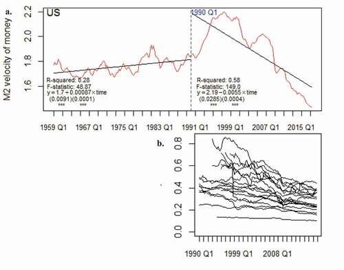
The problem with quantity theory is that a constant increase in velocity is not true anymore. A stable secular increase in velocity prevailed in the United States for the M2 monetary aggregate until approximately 1990. Afterward, the estimated time trend coefficient became significantly negative (Figure 2(a)). The continuation of the decrease in velocity after 2007 can be associated with the preferences of consumers and firms to hold cash instead of spending it, because of the continued low confidence in the recovery after the Great Recession of 2007–09. Similarly, a decreasing trend of M3 velocity was observed in all 20 economies examined from 1990 to 2017 (Figure 2(b)).

Figure 2. Velocity of money

Note: Upper plot (a) presents the M2 velocity of money in the United States from 1Q 1959 to 1Q 2017. Plot (b) presents the M3 velocity of money for the 20 countries examined from 1Q 1990 to 1Q 2017.Source: own work

From 1Q 1990 to 1Q 2017, money growth Granger-caused inflation was observed only in Hungary, Iceland, and South Africa. In Canada and the Czech Republic, the evidence was mixed. In Poland, both variables were endogenous or inflation Granger-caused money growth. In Mexico, both variables were endogenous at the 0.07 significance level (Table 2).

Table 2. Granger causality between money growth (M3) and inflation from 1Q 1990 to 1Q 2017

	M3→CPI, F test and p value			CPI→M3, F test and p value
Country	Method of lag length selection			Method of lag length selection
	AIC	BIC	F tests	AIC	BIC	F tests
Australia	1.54 (0.17)	0.95 (0.39)	1.54 (0.17)	2.82 (0.01)	0.49 (0.62)	2.82 (0.01)
Canada	2.87 (0.01)	2.28 (0.11)	2.87 (0.01)	1.60 (0.14)	1.39 (0.25)	1.60 (0.14)
Switzerland	1.49 (0.17)	1.29 (0.28)	1.49 (0.17)	0.78 (0.62)	1.03 (0.39)	0.78 (0.62)
Chile	1.42(0.22)	1.89 (0.17)	1.42 (0.22)	0.56 (0.73)	0.00 (0.99)	0.56 (0.73)
Czech Republic	1.84 (0.11)	4.57 (0.01)	1.84 (0.11)	0.53 (0.75)	1.53 (0.22)	0.53 (0.75)
Denmark	0.91 (0.48)	0.56 (0.57)	0.91 (0.48)	0.61 (0.69)	0.52 (0.60)	0.61 (0.69)
Euro area	1.78 (0.09)	0.18 (0.84)	1.78 (0.09)	0.99 (0.45)	4.06 (0.02)	0.99 (0.45)
Hungary	2.55 (0.04)	2.55 (0.04)	2.55 (0.04)	1.37 (0.25)	1.37 (0.25)	1.37 (0.25)
Israel	1.81 (0.09)	0.32 (0.57)	1.81 (0.09)	1.21 (0.31)	3.78 (0.05)	1.21 (0.31)
Iceland	2.78 (0.01)	4.75 (0.00)	2.78 (0.01)	0.49 (0.86)	0.97 (0.44)	0.49 (0.86)
Japan	0.82 (0.59)	0.16 (0.69)	0.82 (0.59)	1.20 (0.31)	0.25 (0.62)	1.20 (0.31)
Korea	0.85 (0.56)	0.92 (0.46)	0.85 (0.56)	0.74 (0.65)	0.59 (0.67)	0.74 (0.65)
Mexico	2.87 (0.01)	3.95 (0.01)	2.87 (0.01)	1.92 (0.07)	3.18 (0.02)	1.92 (0.07)
Norway	0.81 (0.55)	0.81 (0.55)	0.81 (0.55)	1.24 (0.30)	1.24 (0.30)	1.24 (0.30)
New Zealand	0.76 (0.62)	2.07 (0.13)	0.45 (0.81)	0.66 (0.71)	2.70 (0.07)	0.96 (0.44)
Poland	0.78 (0.57)	4.72 (0.03)	0.78 (0.57)	3.30 (0.01)	37.90 (.00)	3.30 (0.01)
Sweden	1.21 (0.31)	1.21 (0.31)	1.21 (0.31)	1.93 (0.10)	1.93 (0.10)	1.93 (0.10)
United Kingdom	0.50 (0.84)	1.73 (0.18)	0.83 (0.53)	0.31 (0.95)	1.60 (0.21)	1.11 (0.36)
United States	0.44 (0.85)	0.44 (0.85)	0.44 (0.85)	2.78 (0.02)	2.78 (0.02)	2.78 (0.02)
South Africa	3.00 (0.01)	3.00 (0.01)	3.00 (0.01)	1.30 (0.26)	1.30 (0.26)	1.30 (0.26)

Note: Bold values indicate significance at the 0.05 level, implying a causality running from M3 money supply growth (inflation) to inflation (M3 money supply growth). The statistic of the F test is reported with the corresponding p values in parentheses. The lag order for the Granger causality tests was based on the AIC/BIC criteria and a series of F tests on decreasing lags from eight. For the Granger causality test, the time series were first-differenced if necessary according to the ADF and KPSS tests (Table A1). When the results of the ADF and KPSS tests were ambiguous, I ran an additional ADF-GLS test (Perron-Qu method).

Source: own work

Notwithstanding, proponents of quantity theory might argue that the quantity-like relationship between money growth and inflation will be revealed in the longer run. Instead, for the cycles from 8 (an upper bound of a typical business cycle) to 20 years (Figure 3), the bootstrap correlation coefficient was smaller than 0.3 for more than half of the countries and often negative after 1990 (Table A2). Breuer et al. (2018) explain that the negative correlation in IT can be induced by countervailing shocks to money growth in response to inflation shocks. The study revealed a significant and positive bootstrap correlation coefficient greater than 0.5, but it did not exceed 0.7 in Australia, the Czech Republic, Norway, New Zealand, Iceland, Mexico, and Poland – the latter two countries had high average inflation in my sample of countries.

Nevertheless, except for Poland and Mexico, I failed to reject the null hypotheses of the F test and the bootstrap version of the robust Brown-Forsythe Levene-type test for homogeneity of variances. This finding confirmed the results of the eyeball metric that from 1Q 1990 to 1Q 2017, the long-run money signal typically had (much) greater variance than the long-run changes of inflation. Inflation typically fluctuated around the inflation target. According to the Christiano-Fitzgerald band-pass filter (8–20-year cycle), the signals were not in line with the quantity theory, except for Poland and Mexico (Figure 3, Table A2).

Figure 3. (Continued.)

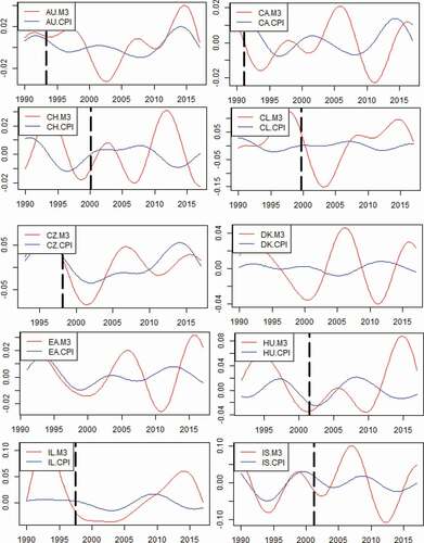
Figure 3. Christiano-Fitzgerald band-pass filter (8–20-year cycle) of M3 growth and inflation from 1Q 1990 to 1Q 2017

Note: The bold dashed line marks the introduction of FFIT. Time series (growth rate same period previous year) were seasonally adjusted before the extraction of a signal.Source: own work

After the Great Recession, the weakening of the quantity theoretic link is even more striking. In many countries, the amplitudes of money growth increased, and inflation remained relatively low in this band (Figure 3). The explanation of low inflation (or even deflation) accompanied by expansionary monetary policy could be the severity of the financial crisis (Mazumder, 2018) that created a permanent output loss (Huang & Luo, 2017). Marcuzzo (2017) argues that the liquidity trap environment in the banking system was responsible for the general deflation despite major central banks’ flooding the markets with liquidity through quantitative easing.

However, a belief could be that the relationship between money growth and inflation might resemble the quantity theory for a cycle from 20 to 40 years. However, the correlation coefficient was nonsignificant in Chile and Norway, whereas it was significantly negative in a relatively large number of countries (the Czech Republic, Hungary, Mexico, New Zealand, the United States, and South Africa). Moreover, except for Switzerland, New Zealand, Poland, and Sweden, the variance of the low-frequency signal of money growth was significantly greater than that of inflation at conventional significance levels. The evidence demonstrates that quantity theoretic relations are difficult to extract even in this band. (Figure A3, Table A2).

For the 2–8-year cycle, the amplitudes of money growth were often much more volatile than stable inflation movements. Only in Mexico, Poland, and South Africa I failed to reject the null hypothesis of the bootstrap Brown-Forsythe test on the homogeneity of variances. In Mexico, however, the correlation coefficient was low and statistically nonsignificant. Thus, Poland and South Africa were the reliable candidates where the short-run quantity-like relationship was significant; in both countries, the phase shift was relatively small; the correlation coefficients were 0.81 and 0.69, respectively; and the relation resembled the quantity theory (Figure 2, Table A2).

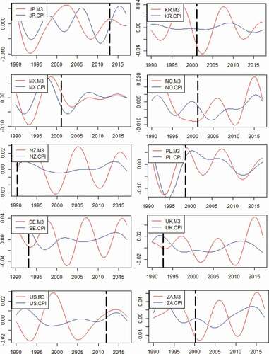
Finally, continuous wavelet analysis provided fresh insights into the discovered interdependencies (Figure 4). The wavelet analysis is significant, because the link changing in time and frequency may be difficult to understand when using the pure frequency-domain or pure time-domain methods (Hkiri, Hammoudeh, Aloui, & Shahbaz, 2018). Compared to the band-pass filters, the value added of the wavelet methodology stems from it not requiring an arbitrary cut-off of the frequency bands. Moreover, the wavelet phase spectrum does not assume a single, one-way link for the whole investigated time span – and this is the case of the conventional Granger causality test (Grinsted et al., 2004).

Figure 4. Wavelet coherency and phase difference between money and inflation from 1Q 1990 to 1Q 2017

Note 1: The frequency unit is a year on the Y axis (up to a 16 years cycle). Time span is on the X axis.

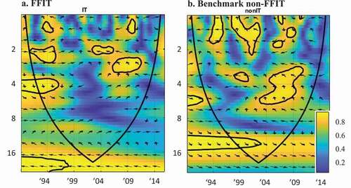
Note 2: If arrows point to the right side, there is a positive instantaneous correlation between money and inflation, if to the left – negative instantaneous correlation, arrows vertically up – money growth leads inflation by exactly π/2, and for arrows vertically down, inflation leads money growth by exactly π/2.

Note 3: Wavelet coherency is marked with colours from blue (no or weak co-movements) to yellow (strong co-movements). The statistically significant estimates of wavelet coherency are marked with black contours.

Note 4: Black U-shaped lines mark the interpretable area (i.e., the cone of influence). The areas outside or overlapping these lines should be interpreted with caution because they might be distorted by zero padding on the boundaries.

Note 5: Input data are seasonally adjusted M3 money and inflation indices (1990 = 100) constructed for the inflation-targeting and benchmark economies and transformed into logarithms.

Source: own work with the use of ASToolbox (Aguiar-Conraria & Soares, 2013) and the cross-wavelet and wavelet coherence toolbox for MATLAB (Grinsted et al., 2004) and own modifications of the codes.

In the short run (less than a 2-year cycle), significant co-movements between money growth and inflation were more frequent in the benchmark countries (Figure 4(b)) than in the sample of full-fledged inflation-targeting regimes (Figure 4(a)). However, the co-movements were typically negative. Evidence of the significant causality running from money growth to inflation appeared before and during the Great Recession of 2007–2009 for a typical business cycle frequency in both groups of countries (Figure 4).

The wavelet results in Figure 4 can be compared to studies that support the relationship between money growth and inflation over the entire period investigated. However, such studies have typically included pre-1990 time series, when the inflation rate was relatively high and volatile (Hossain, 2019a). After 1990, the link between money growth and inflation is argued to have weakened or even broken down (Teles et al., 2016). Indeed, in the Great Moderation era, Sargent and Surico (2011) and Rua (2012) demonstrated the breakdown of the aforementioned relationship in the United States and euro area, respectively. In particular, Rua (2012) finds that the relationship is present until the beginning of the 1980s, at the typical business cycle frequency. From that time on, the leading properties of money growth with respect to inflation continue to deteriorate. The article adds to the aforementioned strand of literature by presenting evidence of a relatively weak link between money growth and inflation from 1990 onwards over the entire investigated period.

The novel finding is that the link might become strong and significant during specific sub-periods, although it may not be significant at normal times. At normal times, the co-movements between money growth and inflation were largely statistically nonsignificant or the direction of causality was not running from money growth to inflation. Instead, the significant link around the Great Recession depicted in Figure 4 can be generally characterized by booming house prices³ and expansionary monetary policy implemented after house prices collapsed.

This finding suggests that a house price boom or expansionary monetary policy might evoke quantity theoretic association. Such an interpretation is in line with studies that have demonstrated that the measured elasticity of prices with respect to money is closer to unity when the money growth is high (Breuer et al., 2018; Gertler & Hofmann, 2018). Thus, the sizable growth of money or credit often precedes asset price booms (Gerdesmeier, Reimers, & Roffia, 2010; Gunn, 2018), which can lead to the subsequent inflationary outburst (Roffia & Zaghini, 2007). The wavelet findings confirm the thesis of Sargent and Surico (2011) that a significant and strong link between money growth and inflation can occur again if monetary authorities allow a persistent, significant increase in money growth. The threat seems to be especially important in the post-crisis environment, when many central banks have started purchasing financial assets at an unconventional (and enormous) scale in response to both the 2007 global financial crisis and the economic slowdown resulting from the COVID-19 pandemic.

The choice of the quarter-on-quarter changes of the CPI and M3 has not affected the general findings (available upon request). From two quarters to the 8-year cycle horizon, the robustness MODWT analysis confirms the relatively weak relationship between money growth and inflation over the entire time span in this band (Table 3).

Table 3. Multiscale correlation of M3 and inflation based on the MODWT from 1Q 1990 to 1Q 2017

Country/region	Frequency scales: quarters, p value in round brackets
	2–4	4–8	8–16	16–32
Australia	0.06 (0.65)	0.09 (0.66)	−0.08 (0.80)	0.10 (0.85)
Canada	−0.14 (0.30)	−0.02 (0.94)	0.48 (0.10)*	0.50 (0.31)
Switzerland	−0.02 (0.91)	−0.24 (0.22)	0.12 (0.69)	−0.06 (0.92)
Chile	0.13 (0.36)	0.18 (0.34)	0.24 (0.42)	0.16 (0.76)
Czech Republic	−0.32 (0.02)**	−0.02 (0.93)	0.18 (0.57)	0.35 (0.50)
Denmark	0.01 (0.92)	0.19 (0.34)	0.12 (0.71)	−0.19 (0.72)
Euro area	−0.16 (0.24)	0.02 (0.92)	0.41 (0.16)	0.48 (0.34)
Hungary	−0.21 (0.14)	−0.40 (0.04)**	−0.11 (0.71)	0.02 (0.97)
Israel	−0.40 (0.002)***	−0.31 (0.11)	−0.08 (0.81)	−0.36 (0.49)
Iceland	−0.09 (0.51)	0.10 (0.62)	0.23 (0.46)	0.48 (0.34)
Japan	−0.07 (0.60)	0.06 (0.76)	0.07 (0.82)	−0.48 (0.35)
South Korea	0.11 (0.43)	0.30 (0.13)	0.34 (0.25)	0.54 (0.26)
Mexico	−0.16 (0.89)	−0.42 (0.16)	−0.10 (0.73)	0.20 (0.71)
Norway	−0.12 (0.40)	−0.13 (0.51)	−0.35 (0.24)	−0.10 (0.85)
New Zealand	0.03 (0.82)	0.29 (0.14)	0.20 (0.51)	0.70 (0.12)
Poland	−0.33 (0.02)**	0.17 (0.39)	0.08 (0.80)	0.41 (0.42)
Sweden	−0.26 (0.06)*	0.10 (0.61)	0.28 (0.35)	0.12 (0.81)
United Kingdom	−0.06 (0.68)	−0.25 (0.21)	−0.04 (0.89)	0.08 (0.88)
United States	−0.13 (0.34)	−0.25 (0.20)	−0.16 (0.59)	0.21 (0.69)
South Africa	0.06 (0.64)	−0.17 (0.40)	0.12 (0.68)	0.49 (0.32)

Note 1: Statistical significance is denoted by the asterisk where *, **, and *** designate the 10%, 5%, and 1% levels of significance, respectively.

Note 2: Input data are seasonally adjusted inflation indices (2010 = 100) and M3 money time series (expressed either as an index or in national currency units, depending on the availability of the data for a given economy), and both are transformed into logarithms.

Source: own work

6. Conclusion

The goal of the article is to assess how far broad money growth and consumer inflation have moved away from quantity theory in full-fledged inflation-targeting regimes since 1990. Recently, some single-country studies, for example, Hossain (2019b) or Ellington and Milas (2019), have documented a strong link between money growth and inflation. By contrast, my findings show that the interconnectedness of money growth and inflation is statistically nonsignificant from 1990 onwards over the entire time span investigated. For the 8–20-year cycle, quantity theory performed relatively well only in Poland and Mexico – both countries had the highest average inflation within the sample considered.

The difficult-to-detect co-movements at normal times may deceive readers into thinking that the link between money growth and inflation is not present or that money is irrelevant. By contrast, the continuous wavelet analysis implies that the quantity theoretic association may occur during specific sub-periods. The study evidenced significant causality running from money growth to inflation, and their strong significant co-movements around the Great Recession at a typical business cycle frequency.

This finding suggests that the quantity theory of money might be revealed at times of expansionary monetary policy or if central banks abandon their primary goal of stabilizing inflation near the target. The interpretation is in line with studies that have demonstrated that the measured elasticity of prices with respect to money is closer to unity when the money growth is high (Breuer et al., 2018; Gertler & Hofmann, 2018). This finding supports the allegation of Sargent and Surico (2011) that a significant, strong link between money growth and inflation can occur again if monetary authorities allow a persistent, significant increase in money growth. The threat seems to be especially important in the post-crisis environment because major central banks have started purchasing financial assets on an unprecedented scale in response to the 2007 global financial crisis and to the economic slowdown resulting from the COVID-19 pandemic.

The significant relationship between the growth rate of the money supply and inflation at a typical business cycle frequency near the Great Recession is of substantial importance for policymakers. Because the long run consists of a series of shorter runs, ignoring surges in money growth that appear in the short run (or especially at the business cycle frequency) may lead to inflation and slower economic growth in the long run. If the longer-run relationship between money growth and inflation begins to take hold, policymakers may need to respond to their past accommodative policy and ignorance about the shorter-run money supply growth by reducing money growth rates in the future. This obviously results in the risks of a recession or – at least – an economic slowdown. Consequently, the article’s empirical findings support the proposal of Taylor (2009) that policymakers should return to a monetary framework that controls the money supply. As Taylor (2009) argues, such a policy seems especially important when nominal interest rates are at their zero lower bound and thus provide little information on the scale of quantitative easing.

In this study, I have not used structural estimation to remain in line with the principal way through which the quantity theory has been advocated. However, the empirical results on the time and frequency-varying linkages between money growth and inflation might be helpful for the construction of post-Great Recession money-augmented models. This approach is important because models without money have neither predicted nor explained the global financial crisis, and the way of including money into macroeconomic models constitutes a challenge (Willen, 2015). The innovative approach to combine the time–frequency perspective with econometric modelling can deliver new implications for the monetary policy. This concept seems particularly valid in the case of the continuous wavelet transform, because the methodology is efficient in identifying damping in dynamic systems (Hkiri et al., 2018; Ramírez & Montejo, 2015).

Disclosure statement

No potential conflict of interest was reported by the author.

Additional information

Funding

The research under the project no. 2017/26/D/HS4/00116 titled: “Money, Credit and House Prices from the Wavelet Perspective” was funded by the National Science Centre, Poland.

Notes

¹ † Australia, Canada, Chile, the Czech Republic, Hungary, Iceland, Israel, South Korea, Mexico, New Zealand, Norway, Poland, South Africa, Sweden, Switzerland, and the United Kingdom. Benchmark economies: Denmark, the Euro area, Japan, the United States.

‡M3 was chosen as a measure of money to retain consistency with the monetary pillar of the European Central Bank.

² US, JP, and the EA are not considered to be FFIT, despite the adopted inflation targets. The Fed operates under a mandate from the Congress to “promote effectively the goals of maximum employment, stable prices, and moderate long term interest rates” – which is commonly referred to as the “dual mandate.” The European Central Bank is not perceived to be a full-fledged inflation targeter due to the adoption of the “two-pillar” monetary policy strategy and a vaguely defined inflation target. According to the speech by Vítor Constâncio, Vice-President of the European Central Bank, at the Conference on “Central Banks in Historical Perspective: What Changed After the Financial Crisis?” on 4 May 2018: “The refusal of pure inflation targeting was justified by the theoretical reason that it did not allow a role for money.” In JP, the new policy framework consists of two components: the first is the “yield curve control” in which the Bank controls short-term and long-term interest rates through market operations; the second one is an “inflation-overshooting commitment” in which the Bank commits itself to expanding the monetary base until the year-on-year rate of increase in the observed CPI exceeds the price stability target of 2 percent and stays above the target in a stable manner – which is far from the principles of full-fledged IT.

³ In the benchmark economies, the emergence of the significant link between money growth and inflation coincides with the beginning of the house price bubbles detected by Ryczkowski (2019).

Appendix

Figure A1. (Continued)

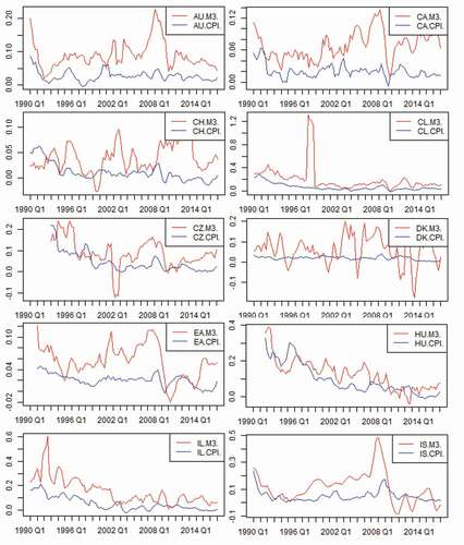
Figure A1. Money growth (M3) and inflation from 1Q 1990 to 1Q 2017

Note: The plot presents annual growth rates from the same quarter of the previous year for seasonally adjusted time series.Source: own work

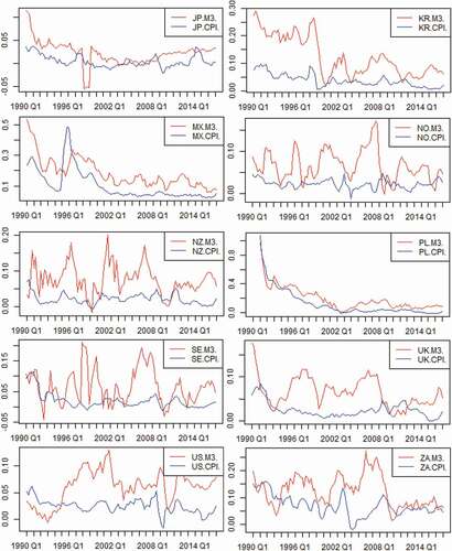
Figure A2. (Continued)

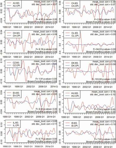
Figure A2. The Christiano-Fitzgerald band-pass filter (2–8 years cycle) of money growth (M3) and inflation from 1Q 1990 to 1Q 2017

Note: The plot presents the band-pass filtered annual growth rates from the same quarter of the previous year for seasonally adjusted time series. The bootstrap methodology was applied to assess the statistical significance of the mean Pearson correlation coefficient [mean_boot.corr.] and its standard deviation [std.dev._boot.corr.] (the number of bootstrap replicates, R = 1,000). Homogeneity of variances of money growth and inflation is tested with a two-tailed F test. The figure also reports the p-values for the robust Brown-Forsythe Levene-type test with the group medians (Lim & Loh, 1996) with 1,000 bootstrap replicates.Source: own work

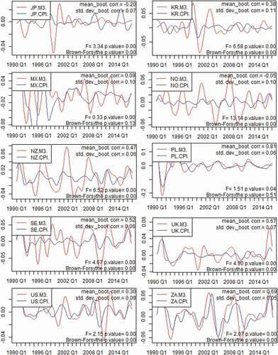
Figure A3. (Continued)

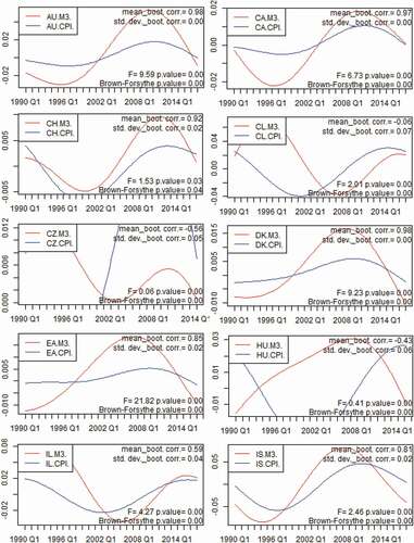
Figure A3. The Christiano-Fitzgerald band-pass filter (20–40 years cycle) and correlation of money growth (M3) and inflation from 1Q 1990 to 1Q 2017

Note: The plot presents the band-pass filtered annual growth rates from the same quarter of the previous year for seasonally adjusted time series. The bootstrap methodology was applied to assess the statistical significance of the mean Pearson correlation coefficient [mean_boot.corr.] and its standard deviation [std.dev._boot.corr.] (the number of bootstrap replicates, R = 1,000). Homogeneity of variances of money growth and inflation is tested with a two-tailed F test. The figure also reports the p-values for the robust Brown-Forsythe Levene-type test with the group medians (Lim & Loh, 1996) with 1,000 bootstrap replicates.Source: own work

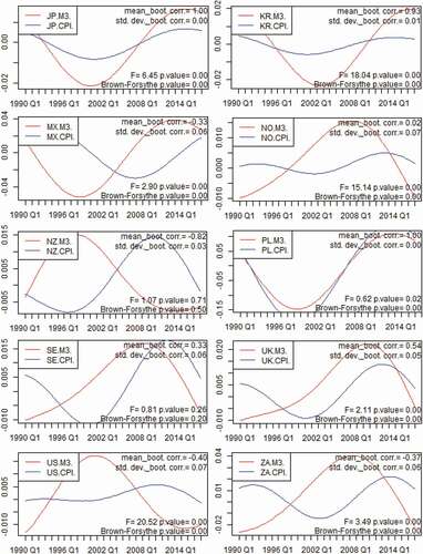
Table A1. KPSS and ADF unit root tests: 1Q 1990–1Q 2017

Symbol	KPSS Test Statistic (.05 Crit. Value:.46.01 Crit. Value:.74)	KPSS Test Statistic including trend (.05 Crit. Value:.15,.01 Crit. Value:.22)	ADF (Test with const.), Test statistic	ADF (Test with const. and trend), Test statistic	Assumed order of integration
AU(CPI)	.09	.07	−8.49(.00)	−8.46(.00)	I(0)
Δ AU(CPI)	.06	.04	−8.12(.00)	−8.08(.00)
AU(M3)	.26	0.2	−3.33(.01)	−3.34(.06)	I(0)
Δ AU(M3)	.02	.03	−7.35(.00)	−7.33(.00)
CA(CPI)	.24	.08	−6.85(.00)	−6.97(.00)	I(0)
Δ CA(CPI)	.05	.03	−6.16(.00)	−6.13(.00)
CA(M3)	.61	.08	−1.84(.36)	−2.58(.29)	I(I)
Δ CA(M3)	.02	.02	−5.67(.00)	−5.63(.00)
CH(CPI)	1.14	.20	−4.17(.00)	−4.85(.00)	I(I)
Δ CH(CPI)	.13	0.04	−5.77(.00)	−6.09(00)
CH(M3)	.29	.07	−3.23(.02)	−3.71(.02)	I(0)
Δ CH(M3)	.03	.03	−3.92(.00)	−3.86(.01)
CL(CPI)	1.21	.39	−3.90(.00)	−4.98(.00)	I(I)
Δ CL(CPI)	.23	.05	−11.34(.00)	−5.61(.00)
CL(M3)	.50	.06	−9.86(.00)	−10.23(.00)	I(0)
Δ CL(M3)	.02	.02	−7.05(.00)	−7.01(.00)
CZ(CPI)	1.21	.25	−3.58(.01)	−4.40(.00)	I(0)
Δ CZ(CPI)	.04	.02	−7.09(.00)	−7.08(.00)
CZ(M3)	.45	.15	−7.80(.00)	−8.11(.00)	I(0)
Δ CZ(M3)	.06	.04	−7.05(.00)	−7.07(.00)
DK(CPI)	.48	.18	−6.55(.00)	−7.03(.00)	I(0)
Δ DK(CPI)	.05	.03	−5.72(.00)	−5.78(.00)
DK(M3)	.06	.06	−4.70(.00)	−4.68(.00)	I(0)
Δ DK(M3)	.04	.03	−8.97(.00)	−8.92(.00)
EA(CPI)	.88	.12	−3.25(.02)	−3.67(.02)	I(0)
Δ EA(CPI)	.04	.03	−4.85(.00)	−4.85(.00)
EA(M3)	.39	.12	−4.26(.00)	−4.11(.01)	I(0)
Δ EA(M3)	.04	.03	−18.74(.00)	−18.74(.00)
HU(CPI)	1.89	.36	−1.93(.32)	−1.84(.68)	I(I)
Δ HU(CPI)	.22	.05	−4.55(.00)	−4.69(.00)
HU(M3)	1.59	.07	−3.02(.03)	−4.47(.00)	I(0)
Δ HU(M3)	.03	.03	−8.51(.00)	−8.66(.00)
IL(CPI)	1.56	.34	−2.19(.21)	−6.03(.00)	I(I)
Δ IL(CPI)	.05	.02	−6.06(.00)	−5.42(.00)
IL(M3)	1.57	.26	−3.14(.02)	−9.28(.00)	I(0)
Δ IL(M3)	.03	.03	−11.38(.00)	−11.7(.00)
IS(CPI)	.16	.16	−1.72(.42)	−2.75(.22)	I(I)
Δ IS(CPI)	.08	.06	−4.29(.00)	−4.27(.00)
IS(M3)	.27	.24	−2.69(.08)	−2.70(.24)	I(I)
Δ IS(M3)	.05	.05	−7.04(.00)	−7.03(.00)
JP(CPI)	.41	.24	−8.14(.00)	−8.30(.00)	I(I)
Δ JP(CPI)	.04	.03	−7.04(.00)	−7.07(.00)
JP(M3)	.46	.34	−9.66(.00)	−9.71(.00)	I(I)
Δ JP(M3)	.06	.03	−7.48(.00)	−6.19(.00)
KR(CPI)	1.32	.14	−2.37(.15)	−8.56(.00)	I(I)
Δ KR(CPI)	.05	.02	−5.68(.00)	−5.72(.00)
KR(M3)	1.45	.19	−2.21(.20)	−3.64(.03)	I(I)
Δ KR(M3)	.04	.03	−4.37(.00)	−4.39(.00)
MX(CPI)	1.24	.13	−2.89(.05)	−4.49(.00)	I(I)
Δ MX(CPI)	.07	.03	−10.18(.00)	−10.17(.00)
MX(M3)	1.61	.13	−2.97(.04)	−4.11(.01)	I(I)
Δ MX(M3)	.05	.03	−8.46(.00)	−8.48(.00)
NO(CPI)	.14	.07	−10.73(.00)	−10.72(.00)	I(0)
Δ NO(CPI)	.03	.03	−7.24(.00)	−6.66(.00)
NO(M3)	.14	.09	−7.24(.00)	−7.28(.00)	I(0)
Δ NO(M3)	.03	.02	−8.15(.00)	−8.12(.00)
NZ(CPI)	.13	.11	−2.61(.09)	−2.6(.28)	I(0)
Δ NZ(CPI)	.04	.03	−6.38(.00)	−6.25(.00)
NZ(M3)	.18	.05	−3.98(.002)	−4.07(.007)	I(0)
Δ NZ(M3)	.03	.03	−8.23(.00)	−8.18(.00)
PL(CPI)	2.10	.51	−3.28(.02)	−1.25(.90)	I(I)
Δ PL(CPI)	1.40	.15	−1.99(.29)	−4.49(.003)
PL(M3)	1.43	.34	−2.8(.057)	−3.48(.041)	I(I)
Δ PL(M3)	.24	.08	−5.29(.00)	−5.23(.00)
SE(CPI)	.70	.21	−7.31(.00)	−7.63(.00)	I(0)
Δ SE(CPI)	.28	.09	−6.30(.00)	−6.42(.00)
SE(M3)	.08	.06	−10.41(.00)	−10.34(.00)	I(0)
Δ SE(M3)	.03	.03	−8.60(.00)	−8.57(.00)
UK(CPI)	.42	.25	−5.78(.00)	−5.25(.00)	I(0)
Δ UK(CPI)	.11	.04	−3.99(.00)	−4.18(.00)
UK(M3)	.52	.11	−2.33(.16)	−4.15(.01)	I(0)
Δ UK(M3)	.07	.06	−3.68(.00)	−3.69(.02)
US(CPI)	.64	.07	−7.69(.00)	−8.08(.00)	I(0)
Δ US(CPI)	.08	.04	−8.28(.00)	−8.27(.00)
US(M3)	.47	.26	−5.73(.00)	−6.01(.00)	I(0)
Δ US(M3)	.04	.04	−8.51(.00)	−8.46(.00)
ZA(CPI)	.79	.23	−2.97(.04)	−3.51(.04)	I(0)
Δ ZA(CPI)	.05	.02	−7.67(.00)	−4.72(.00)
ZA(M3)	.38	.20	−2.59(.09)	−3.45(.04)	I(0)
Δ ZA(M3	.04	.03	−4.39(.00)	−4.54(.00)

Asymptotic p-values for the ADF test are in round brackets. The Akaike Criterion was used to indicate the lag length. A lag of 12 quarters was selected and tested down from the maximum lag order. When the results of the ADF and KPSS tests were ambiguous, an ADF-GLS test (Perron-Qu method) was performed at 0.05 level.

Source: own work

Table A2. The correlation coefficients and the F-tests of M3 growth and inflation for the 2–8 years cycle, 8–20 years cycle, and 20–80 years cycle from 1Q 1990 to 1Q 2017

	CC and its SD	F test	CC and its SD	F test	CC and its SD	F test
Country	2–8 years cycle		8–20 years cycle		20–80 years cycle
Australia	0.57 (0.07)	4.95	0.51 (0.07)	4.87	0.98 (0.00)	9.59
Canada	0.39 (0.07)	2.88	−0.10 (0.08)	2.94	0.97 (0.00)	6.73
Switzerland	−0.05 (0.09)	9.19	−0.18 (0.08)	5.98	0.92 (0.02)	1.53
Chile	0.14 (0.05)	94.63	−0.37 (0.05)	34.69	−0.06 (0.07)	2.01
Czech Republic	0.41 (0.08)	1.91	0.66 (0.06)	2.24	−0.56 (0.05)	0.06
Denmark	0.10 (0.08)	103.66	−0.53 (0.07)	35.15	0.98 (0.00)	9.23
Euro area	0.68 (0.05)	8.83	0.29 (0.08)	6.22	0.85 (0.02)	21.82
Hungary	−0.16 (0.10)	5.04	−0.16 (0.10)	7.59	−0.43 (0.06)	0.41
Israel	0.05 (0.11)	6.71	0.37 (0.06)	23.34	0.59 (0.04)	4.27
Iceland	0.31 (0.10)	7.91	0.58 (0.04)	6.79	0.81 (0.02)	2.46
Japan	−0.20 (0.07)	3.34	0.31 (0.08)	1.50	1.00 (0.00)	6.45
Korea	0.38 (0.11)	6.58	0.21 (0.07)	26.42	0.93 (0.01)	18.04
Mexico	0.09 (0.10)	0.33	0.65 (0.05)	1.28	−0.33 (0.06)	2.90
Norway	−0.05 (0.10)	13.14	0.52 (0.07)	4.29	0.02 (0.07)	15.14
New Zealand	0.47 (0.06)	6.52	0.50 (0.06)	16.14	−0.82 (0.03)	1.07
Poland	0.81 (0.06)	1.51	0.70 (0.05)	1.03	1.00 (0.00)	0.62
Sweden	0.52 (0.06)	4.67	−0.25 (0.06)	4.57	0.33 (0.06)	0.81
United Kingdom	0.67 (0.07)	4.90	−0.09 (0.07)	5.48	0.54 (0.05)	2.11
United States	0.30 (0.09)	2.15	−0.51 (0.07)	8.02	−0.40 (0.07)	20.52
South Africa	0.69 (0.05)	2.07	0.13 (0.07)	2.86	−0.37 (0.06)	3.49

The table presents estimates of the correlation coefficient (CC), its standard deviation (SD) and F test for the signals of M3 growth and inflation from Figures 3, A2 and A3 using bootstrapping method with 1,000 bootstrap replicates. Homogeneity of variances of money growth and inflation is tested with a two-tailed F test. SD is presented in parentheses.

Source: own work

References

- Aguiar-Conraria, L., & Soares, M. J. (2013). The continuous wavelet transform: Moving beyond uni- and bivariate analysis. Journal of Economic Surveys, 28(2), 344–375.
- Avdjiev, S., Koch, C., McGuire, P., & von Peter, G. (2018). Transmission of monetary policy through global banks: Whose policy matters? Journal of International Money and Finance, 89, 67–82.
- Bacchetta, P., Benhima, K., & Kalantzis, Y. (2019). Money and capital in a persistent liquidity trap. Journal of Monetary Economics. doi:https://doi.org/10.1016/j.jmoneco.2019.09.005
- Belongia, M. T., & Ireland, P. N. (2018). Targeting constant money growth at the zero lower bound. International Journal of Central Banking, 2, 159–204.
- Berentsen, A., Huber, S., & Marchesiani, A. (2015). Financial innovations, money demand, and the welfare cost of inflation. Journal of Money, Credit and Banking, 47(S2), 223–261.
- Boehlke, J., Faldzinski, M., Galecki, M., & Osinska, M. (2020). Searching for factors of accelerated economic growth: The case of Ireland and Turkey. European Research Studies Journal, XXIII(Issue 1), 292–304.
- Borio, C. E. V., & Filardo, A. (2007). Globalisation and inflation: New cross-country evidence on the global determinants of domestic inflation (BIS Working Paper No. 227).
- Breuer, J. B., Mcdermott, J., & Weber, W. E. (2018). Time aggregation and the relationship between inflation and money growth. Journal of Money, Credit and Banking, 50(2–3), 351–375.
- Bugamelli, M., Fabiani, S., & Sette, E. (2015). The Age of the dragon: The effect of imports from China on firm-level prices. Journal Of Money, Credit & Banking (Wiley-Blackwell), 47(6), 1091–1118.
- Buiter, W. H. (2000). Monetary misconceptions: New and old paradigmata and other sad tales (CEPR Discussion Paper No. 2365).
- Christev, A., & Kang, Y. (2015). Money and inflation: Is monetary policy useful? The Manchester School, 83, 30–50.
- Christiano, L. J., & Fitzgerald, T. J. (2003). The band pass filter*. International Economic Review, 44(2), 435–465.
- Ciżkowicz, P., & Rzońca, A. (2017). Are major central banks blinded by the analytical elegance of their models? Possible costs of unconventional monetary policy measures. The Singapore Economic Review, 62(1), 87–108.
- Clive, W. J., & Lin, J.-L. (1995). Causality in the long run. Econometric Theory, 11(3), 530–536.
- Cooray, A., & Khraief, N. (2019). Money growth and inflation: New evidence from a nonlinear and asymmetric analysis. The Manchester School, 87(4), 543–577.
- De Santis, R. A. (2015). Quantity theory is alive: The role of international portfolio shifts. Empirical Economics, 49(4), 1401–1430.
- Debortoli, D., Kim, J., Lindé, J., & Nunes, R. (2019). Designing a simple loss function for central banks: Does a dual mandate make sense? The Economic Journal, 129(621), 2010–2038.
- Edquist, H., & Henrekson, M. (2017). Do R&D and ICT affect total factor productivity growth differently? Telecommunications Policy, 41(2), 106–119.
- Ellington, M., & Milas, C. (2019). Global liquidity, money growth and UK inflation. Journal of Financial Stability, 42, 67–74.
- Fanta, F. (2013). Financial deregulation, economic uncertainty and the stability of money demand in Australia. Economic Papers: A Journal of Applied Economics and Policy, 32(4), 496–511.
- Fedotenkov, I. (2018). Population ageing and inflation with endogenous money creation. Research in Economics, 72(3), 392–403.
- Gerdesmeier, D., Reimers, H., & Roffia, B. (2010). Asset price misalignments and the role of money and credit. International Finance, 13(3), 377–407.
- Gertler, P., & Hofmann, B. (2018). Monetary facts revisited. Journal of International Money and Finance, 86, 154–170.
- Giraud, G., & Pottier, A. (2016). Debt-deflation versus the liquidity trap: The dilemma of nonconventional monetary policy. Economic Theory, 62(1/2), 383–408.
- Grauwe, P. D., & Polan, M. (2014). Is Inflation always and everywhere a monetary phenomenon? Exchange Rates and Global Financial Policies, 357–382. doi:https://doi.org/10.1142/9789814513197_0014
- Grinsted, A. J., Moore, C., & Jevrejeva, S. (2004). Application of the cross wavelet transform and wavelet coherence to geophysical time series. Nonlinear Processes in Geophysics., 11(5–6), 561–566.
- Gunn, C. M. (2018). Overaccumulation, interest, and prices. Journal of Money, Credit and Banking, 50(2–3), 479–511.
- Haug, A. A., & Dewald, W. G. (2011). Money, output, and inflation in the longer term: Major industrial countries, 1880–2001. Economic Inquiry, 50(3), 773–787.
- Hkiri, B., Hammoudeh, S., Aloui, C., & Shahbaz, M. (2018). The interconnections between U.S. financial CDS spreads and control variables: New evidence using partial and multivariate wavelet coherences. International Review of Economics & Finance, 57, 237–257.
- Hohberger, S., Priftis, R., & Vogel, L. (2019). The macroeconomic effects of quantitative easing in the euro area: Evidence from an estimated DSGE model. Journal of Economic Dynamics and Control, 108, 103756.
- Hossain, A. A. (2019a). Does money have a role in the inflation process? Evidence from Australia. Australian Economic Papers,58(2), 113–129.
- Hossain, A. A. (2019b). How justified is abandoning money in the conduct of monetary policy in Australia on the grounds of instability in the money‐demand function? Economic Notes, 48(2).
- Huang, Y.-F., & Luo, S. (2017). Potential output and inflation dynamics after the Great recession. Empirical Economics, 55(2), 495–517.
- Itaya, J.-I., & Mino, K. (2007). Technology, preference structure, and the growth effect of money supply. Macroeconomic Dynamics, 11(5), 589–612.
- Jiang, C., Chang, T., & Li, X.-L. (2015). Money growth and inflation in China: New evidence from a wavelet analysis. International Review of Economics & Finance, 35, 249–261.
- Kočenda, E., & Varga, B. (2018). The impact of monetary strategies on inflation persistence. International Journal of Central Banking, 14(4), 229–274.
- Lim, T.-S., & Loh, W.-Y. (1996). A comparison of tests of equality of variances. Computational Statistics & Data Analysis, 22(3), 287–301.
- Liu, J., & Kool, C. J. M. (2018). Money and credit overhang in the euro area. Economic Modelling, 68, 622–633.
- Long, X., Goswami, M., & Jobst, A. (2009). An investigation of some macro-financial linkages of securitization (IMF Working Papers 09(26)). doi:https://doi.org/10.5089/9781451871739.001
- Marcuzzo, M. C. (2017). The “Cambridge” critique of the quantity theory of money: A note on how quantitative easing vindicates it. Journal of Post Keynesian Economics, 40(2), 260–271.
- Matousek, R., Papadamou, S. Τ., Šević, A., & Tzeremes, N. G. (2019). The effectiveness of quantitative easing: Evidence from Japan. Journal of International Money and Finance, 99, 102068.
- Mazumder, S. (2018). Inflation in Europe after the great recession. Economic Modelling, 71, 202–213.
- McLeay, M., Radia, A., & Thomas, R. (2014). Money creation in the modern economy. Bank Of England Quarterly Bulletin, 54(1), 14–27.
- Morana, C. (2006). A small scale macroeconometric model for the Euro-12 area. Economic Modelling, 23(3), 391–426.
- Nunes, A. B., St. Aubyn, M., Valério, N., & de Sousa, R. M. (2018). Determinants of the income velocity of money in Portugal: 1891–1998. Portuguese Economic Journal, 17(2), 99–115.
- Ramírez, R. I., & Montejo, L. A. (2015). On the identification of damping from non-stationary free decay signals using modern signal processing techniques. International Journal of Advanced Structural Engineering (IJASE), 7(3), 321–328.
- Roffia, B., & Zaghini, A. (2007). Excess money growth and inflation dynamics*. International Finance, 10(3), 241–280.
- Roger, M. S., & Stone, M. M. R. (2005). On target? The international experience with achieving inflation targets (No. 5–163). International Monetary Fund.
- Rua, A. (2012). Money Growth and inflation in the Euro area: A time-frequency view. Oxford Bulletin Of Economics & Statistics, 74(6), 875–885.
- Ryczkowski, M. (2017). Forward guidance, pros, cons and credibility. Prague Economic Papers, 26(5), 523–541.
- Ryczkowski, M. (2019). Money, credit, house prices and quantitative easing – The wavelet perspective from 1970 to 2016. Journal of Business Economics and Management, 20(3), 546–572.
- Ryczkowski, M. (2020). Money and credit during normal times and house price booms: Evidence from time-frequency analysis. Empirica, 47(4), 835–861.
- Sargent, T., & Surico, P. (2011). Two illustrations of the quantity theory of money: Breakdowns and revivals. The American Economic Review, 101(1), 113–132.
- Schularick, M., & Taylor, A. M. (2012). Credit booms gone bust: monetary policy, leverage cycles, and financial crises, 1870–2008. American Economic Review, 102(2), 1029–1061.
- Sławiński, A. (2019). The divergence between actual central banking and conventional economics. Argumenta Oeconomica, 1(42), 5–20.
- Stock, J. H., & Watson, M. W. (2007). Why has U.S. Inflation become harder to forecast? Journal of Money, Credit and Banking, 39(s1), 3–33.
- Taylor, J. B. (2009). The need to return to a monetary framework. Business Economics, 44(2), 63–72.
- Taylor, J. B. (2019). Inflation targeting in high inflation emerging economies: Lessons about rules and instruments. Journal of Applied Economics, 22(1), 102–115.
- Teles, P., Uhlig, H., & Azevedo, J. V. (2016). Is quantity theory still alive? The Economic Journal, 126(591), 442–464.
- Temizsoy, A., & Montes-Rojas, G. (2019). Measuring the effect of monetary shocks on European sovereign country risk: An application of GVAR models. Journal of Applied Economics, 22(1), 484–503.
- Temple, J. (2002). Openness, inflation, and the Phillips curve: A puzzle. Journal of Money, Credit, and Banking, 34(2), 450–468.
- Torrence, C., & Compo, G. P. (1998). A practical guide to wavelet analysis. Bulletin of the American Meteorological Society, 79(1), 61–78.
- van den End, J. W. (2016). Quantitative easing tilts the balance between monetary and macroprudential policy. Applied Economics Letters, 23(10), 743–746.
- Vandenberghe, V. (2017). The productivity challenge. What to expect from better-quality labour and capital inputs? Applied Economics, 49(40), 4013–4025.
- Whitcher, B., Guttorp, P., & Percival, D. B. (2000). Wavelet analysis of covariance with application to atmospheric time series. Journal of Geophysical Research: Atmospheres, 105(D11), 14941–14962.
- Willen, P. (2015). Discussion of Arslan, Guler, and Taskin. Journal of Money, Credit and Banking, 47(S1), 171–174.
- Zhang, C. (2017). The great globalization and changing inflation dynamics. International Journal of Central Banking, 13(4), 191–226.