Value-at-risk in the presence of asset price bubbles

ABSTRACT

In this study, we respond to the criticism that the value-at-risk (VaR) measure fails during financial crises and is only applicable during periods without asset price bubbles. We propose a new dating mechanism that is based on the work of Phillips (2015) to date-stamp the origination and termination of the asset price bubbles. Our method relaxed the minimum bubble duration constraint in the original model, and the empirical application statistically identified the bubbles periods in nine stock markets (Australia, Canada, China, Germany, Spain, Hong Kong, Japan, the United Kingdom, and the United States). We choose the two most widely adopted VaR models (RiskMetrics and RiskMetrics 2006) to test the performance. Our results show that the RiskMetrics model fails in most periods, whereas the RiskMetrics 2006 performs efficiently in the periods with asset price bubbles. These results prove the criticism that all the VaR models fail during crises as invalid.

KEYWORDS:

• Asset price bubbles
• value-at-risk
• financial crisis
• date-stamping bubbles

1. Introduction

Financial markets have experienced several crises over the last two decades. The Asian financial crisis in 1997, the dot-com bubble burst in 2001, the subprime mortgage crisis in 2008, and the European sovereign debt crisis in 2009 have driven the financial institutions to use better measures to manage downside risk. The losses caused by these financial crises were tremendous; the 2008 subprime mortgage crisis costed the US economy up to 14 USD trillion (Atkinson, Luttrell, & Rosenblum, 2013), which is equivalent to the average annual output of the entire US economy. Furthermore, the global economy has become more integrated and the cross-border financial flows have steadily increased. This widens the contagion effect and complicates the effects of the financial crisis further.

Financial crises are predominantly caused by the burst of asset price bubbles. An asset price bubble is formed when the asset’s price deviates from its fundamental value. During the bubble booming period, an asset’s price grows at an explosive rate. Blanchard and Watson (1982) suggest that asset bubbles last only till the market realizes it and makes corrections. The correction is usually associated with a large sale force that causes a plunge in the stock price. This process is commonly referred as a bubble burst. However, it is difficult to identify bubbles and date-stamp the bursts.

The losses from the financial crises have led the practitioners and regulators to actively look for risk models that measure the downside risks. Over the past decade, value-at-risk (VaR) has emerged as one of the most popular methods for measuring the downside risks of financial investments. The downside risk of a financial investment predicts the minimum loss of a portfolio’s value for a period with a certain probability. After the subprime mortgage crisis in 2008, practitioners and regulators criticised the VaR models for failing to reveal the underlying risk, which led many financial institutions to suffer unexpected losses well above the VaR value and resulted in a credit crunch. However, most criticism stems from the lack of statistical analysis, which leads to false conclusions on the efficiency of VaR models.

Although a considerable body of research criticises VaR for performing poorly during turbulent financial periods (see Mertzanis, 2013; Lockwood, 2015), most literature classifies crisis and non-crisis periods unclearly by its own subjective judgment. Halbleib and Pohlmeier (2012) proposed a data-driven VaR method that combines quantile forecasts to improve VaR’s performance during a crisis. They formed three portfolios to represent small-, middle-, and large-cap stocks in the Dow Jones index and evaluated the performance in the claim period (1 January 2007 to 17 July 2007), crisis period (18 July 2007 to 1 July 2009), and crash period (1 September 2008 to 1 July 2009). The results show that the method performs well in the crisis periods. However, the crisis and non-crisis periods were defined arbitrarily without a statistical basis. Chen, Gerlach, Lin, and Lee (2012) studied the RiskMetrics models (Riskmetrics, 1996) and several generalised autoregressive conditional heteroscedasticity (GARCH) (Bollerslev, 1986) family VaR models under Bayesian forecasting tests in Japan, Hong Kong, Korea, and the US markets. Their study ranks the RiskMetrics model last among all models, and shows that all VaR models underestimate the risk level during a crisis period. However, similar to the work of Halbleib and Pohlmeier (2012), the crisis and non-crisis periods were defined arbitrarily and the crisis periods were considered to be the same across different stock markets with different characteristics, which is debatable.

Our study contributes to the literature that responds to these limitations, by empirically testing the VaR models’ performance in periods with and without asset price bubbles, particularly in the periods of financial crisis after the bubbles burst. Against the background of criticism for VaR models, we perform a series of backtests to statistically evaluate its performance. Following Phillips, Shi, and Yu (2015), we use the backward supremum augmented Dickey–Fuller (BSADF) test to date-stamp the origination and termination of the bubbles. However, we modify the date-stamping algorithm to suit backtesting. We define three periods for the tests: the pre-bubble period, bubble period, and post-burst period. The bubble period is bounded by the bubble’s origination and termination dates and the pre- and post-burst periods are defined as 2 years before and 2 years after the termination date, respectively. Our date-stamping method allows researchers to evaluate the financial models that may behave differently at different stages of a bubble.

Though VaR is a popular means to quantify downside risk, there is little consensus on the preferred VaR model. Köksal and Orhan (2013) tested a VaR model based on a simple autoregressive conditional heteroscedasticity (ARCH) setting in the developed and emerging markets during financial crisis. Their results show that VaR performs more inefficiently in developed countries than in emerging countries and, overall, fails to reveal the downside risk. However, their results may only be true for the ARCH-based VaR model. Bams, Blanchard, and Lehnert (2017) compared VaR’s performance in the S&P 500, Dow Jones Industrial Average, and Nasdaq 100 indices. The results show that the VaR based on historical volatility measure outperforms other parametric VaR models. Lee, Chiou, and Lin (2006) employed Engle (2002) dynamic conditional correlation (DCC) estimators to estimate a portfolio’s VaR. The authors found that VaR performance at a portfolio level may be unreliable due to the difficulty in forecasting the dynamic correlation among assets. For better modeling of a portfolio’s volatility, Chiriac and Voev (2011) developed a multivariate vector fractionally integrated ARMA (VARFIMA) process that models the long memory characteristics of financial volatility. Furthermore, Engle, Ledoit, and Wolf (2019) proposed a new standard of DCC model that applies nonlinear shrinkage in the estimation of the portfolios of large dimensions. Recent studies such as Fiszeder, Fałdziński, and Molnár (2019) and Law, Li, and Yu (2020) incorporate the state-of-the-art volatility estimation method in the calculation of portfolio VaR. The results show that the choice of volatility model significantly impacts the accuracy of the VaR estimates.

We follow Campbell and Shiller (1989) and Phillips et al. (2015) to consider the explosive behaviour in log price–dividend ratio for the detection of asset price bubble. To understand the VaR performance in different markets, we examine nine stock markets (Australia, Canada, China, Germany, Spain, Hong Kong, Japan, the UK, and the US, and proxy each of the market portfolios by its respective market index. In light of this, our analysis focuses on univariate VaR models and uses the two widely adopted univariate VaR models – RiskMetrics (Riskmetrics, 1996) and RiskMetrics 2006 (Zumbach, 2007) – in our empirical tests in response to the criticism of VaR failure. To evaluate the performance of the VaR models in different periods, we conduct the unconditional coverage tests (Kupiec, 1995), the independence tests (Christoffersen & Pelletier, 2004), and the joint coverage tests. The empirical results of both the conditional and unconditional coverage tests suggested that the RiskMetrics 2006 model adequately described the downside risks in all the nine markets during the bubble periods. However, one weakness noted in the RiskMetrics 2006 model was its tendency to occasionally overstate the downside risk after a market turbulence. Further, the RiskMetrics 2006 model reported zero VaR violations in post-burst periods in Australia, Canada, Japan, and the UK. The empirical results of the conditional coverage tests, unconditional coverage tests, and Fisher’s exact tests suggested that the RiskMetrics 2006 model performs efficiently in most periods, rendering the criticism against VaR models statistically invalid.

The remainder of this paper is organised as follows: Section 2 discusses the rationale of using the log price/dividend ratio as an indicator of asset price bubbles. Section 3 explains the SADF and generalised SADF (GSADF) tests used to identify asset price bubbles and the date-stamping mechanism. Section 4 describes the RiskMetrics and RiskMetrics 2006 VaR models, as well as the backtesting methods. The empirical results of the GSADF tests, identification of the bubble periods, and VaR backtesting results for the sample markets are presented in Section 5. Section 6 concludes the study.

2. Asset prices and bubbles

Asset price bubbles are usually driven by speculative behaviours that bid up the asset prices beyond their fundamental values. The fundamental value of an asset is the sum of the discounted future cash flows. In the presence of bubbles, asset prices behave explosively. The log price of a security is defined as

(1) $p_t=p_t^f+b_t,$(1)

where $p_t$ is the log price at a time $\mathit{t}$, $p_t^f$ is the fundamental value, and $b_t$ is the bubble component (Campbell & Shiller, 1989).

In this equation 1(1) $p_t=p_t^f+b_t,$(1) , the value of $p_t^f$ is the fundamental component of the stock price as it depends on the expected dividends. In contrast, $b_t$ is the speculative component as it is based on the future expectations on the stock price. The stock price will be explosive if the bubble component $b_t$ in the equation 1(1) $p_t=p_t^f+b_t,$(1) is non-zero.

The log price–dividend ratio is the summation of a series of log dividend differences and the bubble components (Campbell & Shiller, 1989; Phillips et al., 2015). If the log dividend is stationary after differencing, an explosive behaviour of the log price–dividend ratio would be caused by the presence of a non-zero bubble component $b_t$. Thus, we can detect if asset price bubbles exist by examining any explosive behaviour in the log price–dividend ratio series and non-explosive behaviour in the first difference log dividend series.

3. SADF and GSADF tests

Previous studies have suggested using a supremum of a set of recursive right-tailed augmented Dickey–Fuller (ADF) tests to detect the presence of stock bubbles (Dickey & Fuller, 1979). This SADF test applies the right-tailed ADF test with the null hypothesis of a unit root ($\mathit{\varphi }=0$) and the alternative hypothesis of an explosive root ($\mathit{\varphi }>0$).

The regression model used in the SADF test is

(2) $\mathrm{\Delta }{y}_t=\mathit{\alpha }+\mathit{\pi }{y}_{\mathit{t}-1}+\sum _{\mathit{j}=1}^k{\gamma }_j\mathrm{\Delta }{y}_{\mathit{t}-\mathit{j}}+{\in }_t,$(2)

where $\mathit{k}$ is the lag order and ${\in }_t$ is the random error.

The SADF test begins with testing the first $r_0$ fraction of the observations. It is followed by repeated ADF tests till $r_0$ is increased to 1, which is denoted by $\mathit{AD}{F}_{r_0}^1$. The forward sequence of the regression starts from observation 1 and ends with $\lfloor \mathit{T}{r}_w\rfloor$, where $\lfloor .\rfloor$ is the integer part of the argument, $\mathit{T}$ is the total number of observations, and $r_w\in [r_0,1]$ is the fraction of the observations. The SADF statistic is

$\mathit{SAD}{F}_{r_0}=\underset{r_w\in [r_0,1]}{sup}\mathit{AD}{F}_0^{r_w}.$

The corresponding asymptotic distribution of the SADF test is discussed by Phillips, Shi, and Yu (2014). The asymptotic distribution of the SADF test statistic for the null hypothesis that the true process is a random walk without drift is

(3) $\mathit{SAD}{F}_{r_0}\to \underset{r_w\in [r_0,1]}{sup}\left\{\frac{r_w[{\int }_0^{r_w}\mathit{WdW}-1/2r_w]-\mathit{W}(r_w){\int }_0^{r_w}\mathit{Wdr}}{r_w^{1/2}{\{r_w{\int }_0^{r_w}{W}^2\mathit{dr}-{[{\int }_0^{r_w}\mathit{W}(\mathit{r})\mathit{dr}]}^2\}}^{1/2}}\right\},$(3)

where $\mathit{W}$ is a Wiener process.

We determine if the behaviour of the data series is explosive by comparing the SADF statistic of the data series with the asymptotic distribution of the Dickey–Fuller t-statistic in equation 3(3) $\mathit{SAD}{F}_{r_0}\to \underset{r_w\in [r_0,1]}{sup}\left\{\frac{r_w[{\int }_0^{r_w}\mathit{WdW}-1/2r_w]-\mathit{W}(r_w){\int }_0^{r_w}\mathit{Wdr}}{r_w^{1/2}{\{r_w{\int }_0^{r_w}{W}^2\mathit{dr}-{[{\int }_0^{r_w}\mathit{W}(\mathit{r})\mathit{dr}]}^2\}}^{1/2}}\right\},$(3) . We perform a backward ADF (BADF) test to date-stamp the explosion. The BADF test performs the ADF test repeatedly by fixing the starting point of the sample at the first observation, and rolling the ending point from $\lfloor {\mathit{Tr}}_0\rfloor$ to $\mathit{T}$. For example, if the testing sequence starts from $r_1$ ($r_1=0$ in the BADF test) and ends at $r_2$, the corresponding BADF test statistic would be $\mathit{BAD}{F}_{r_1}{r}_2$. The BADF test statistic is denoted by $\mathit{BAD}{F}_{r_2}$ because the first observation is the starting point.

The explosion originates at $\lfloor \mathit{T}{r}_e\rfloor$ when it is the first occurrence after the $\mathit{BAD}{F}_{r_e}$ statistic exceeds the critical value. Phillips, Wu, and Yu (2011) impose the conditions that the bubble duration must be longer than $\mathit{log}(\mathit{T})$ and the termination date of the explosion ($\lfloor \mathit{T}{r}_f\rfloor$) must be the first occurrence after the observation $\lfloor \mathit{T}{r}_e\rfloor +\mathit{log}(\mathit{T})$, when the $\mathit{BAD}{F}_{r_f}$ statistic is below the critical value.

(4a) $r_e=\underset{r_2\in [r_0,1]}{inf}\{r_2:\mathit{BAD}{F}_{r_2}>\mathit{c}{v}_{r_2}^{{\beta }_T}\}$(4a)

(4b) $r_f=\underset{r_2\in [{\hat{r}}_{\mathit{e}}+\mathit{\delta }\frac{\mathit{log}(\mathit{T})}{T},1]}{inf}\{r_2:\mathit{BAD}{F}_{r_2}<\mathit{c}{v}_{r_2}^{{\beta }_T}\}$(4b)

Phillips et al. (2011) further recommended that the critical value $\mathit{c}{v}_{r_2}^{{\beta }_T}$ should vary with the number of observations in the testing window for it to diverge to infinity and eliminate type I errors for large $\mathit{T}$; specifically, they suggested setting $\mathit{c}{v}_{r_2}^{{\beta }_T}=\mathit{log}(\mathit{log}(\mathit{T}{r}_s))/100$. The test using the bubble date-stamping method of equation 4 is referred to as the PWY test in this paper.

The disadvantage of the PWY test is the possible failure when multiple bubbles are present in the sample. Phillips et al. (2015) proposed the generalised version of SADF (i.e., the GSADF test) to address this issue for its flexibility in allowing changes to the starting point of the testing window. The GSADF statistic is defined as

$\mathit{GSAD}{F}_{r_0}=\underset{r_w\in [r_0,1]}{sup}\{\mathit{su}{p}_{r_1\in [0,1-r_w]}\mathit{AD}{F}_{r_1}^{r_w}\}.$

The asymptotic distribution of the GSADF test is elaborated by Phillips et al. (2014).

The date-stamping method used in the GSADF test is an extended version of the one used in the BADF statistic. The BSADF test performs an SADF test by rolling the starting point of the test window $r_1\in [0,r_2-r_0]$ from observation $⌊\mathit{T}(r_2-r_0)⌋$ to the first observation. The BSADF statistic for a testing sequence that starts at $r_1$ and ends at $r_2$ is defined as

$\mathit{BSAD}{F}_{r_2}=\underset{r_1\in [0,r_2-r_0]}{sup}\mathit{BAD}{F}_{r_1}{r}_2.$

Similar to the PWY test, the origination date of a bubble in the GSADF test is $⌊\mathit{T}{\hat{r}}_{\mathit{e}}⌋$, when $⌊\mathit{T}{\hat{r}}_{\mathit{e}}⌋$ is the first occurrence after the $\mathit{BSAD}{F}_{{\hat{r}}_{\mathit{e}}}$ statistic exceeds the critical value. The minimum bubble duration in the BSADF statistic is generalised to $\mathit{\delta log}(\mathit{T})$, where $\mathit{\delta }$ is a frequency-dependent parameter. Furthermore, the termination date of explosion $⌊\mathit{T}{\hat{r}}_{\mathit{f}}⌋$ is the first occurrence after the observation $⌊\mathit{T}{\hat{r}}_{\mathit{e}}+\mathit{\delta log}(\mathit{T})⌋$, when the $\mathit{BSAD}{F}_{r_2}$ statistic is below the critical value. The bubble date-stamping method of equation 5 is referred to as the PSY test in this paper.

(5a) ${\hat{r}}_{\mathit{e}}=\underset{r_2\in [r_0,1]}{inf}\left\{r_2:\mathit{BSAD}{F}_{r_2}>\mathit{c}{v}_{r_2}^{{\beta }_T}\right\}$(5a)

(5b) ${\hat{r}}_{\mathit{f}}=\underset{r_2\in [{\hat{r}}_{\mathit{e}}+\mathit{\delta }\frac{\mathit{log}(\mathit{T})}{T},1]}{inf}\left\{r_2:\mathit{BSAD}{F}_{r_2}<\mathit{c}{v}_{r_2}^{{\beta }_T}\right\}$(5b)

The bubble origination date in the GSADF test is date-stamped using equation 5a(5a) ${\hat{r}}_{\mathit{e}}=\underset{r_2\in [r_0,1]}{inf}\left\{r_2:\mathit{BSAD}{F}_{r_2}>\mathit{c}{v}_{r_2}^{{\beta }_T}\right\}$(5a) , which is the ending point $r_2$ of the testing window in the BSADF statistic. The PSY date-stamping method picks the ending point in an explosive series as the bubble origination date. Though this gives confidence in forward tests, it might miss the bubble formation period, which is crucial for a backtest. Alternately, we examine the bubble origination date by considering the starting point as $r_1$ instead of $r_2$ of the explosive series. Thereby, we modify the date-stamping method for the bubble origination date as in equation 6a(6a) ${\bar{r}}_{\mathit{e}};{\bar{r}}_2=\underset{r_2\in [r_0,1]}{inf}\left\{r_1;r_2:\mathit{BSAD}{F}_{r_2}>\mathit{c}{v}_{r_2}^{{\beta }_T}\right\}$(6a) . The new bubble origination date is $⌊\mathit{T}{\bar{r}}_{\mathit{e}}⌋$. ${\bar{r}}_2$, in equation 6a(6a) ${\bar{r}}_{\mathit{e}};{\bar{r}}_2=\underset{r_2\in [r_0,1]}{inf}\left\{r_1;r_2:\mathit{BSAD}{F}_{r_2}>\mathit{c}{v}_{r_2}^{{\beta }_T}\right\}$(6a) , is the end of the testing sequence in the BSADF test for bubble origination. We use this ending point as a starting point to detect the termination date of the explosion $⌊\mathit{T}{\bar{r}}_{\mathit{f}}⌋$ in equation 6b(6b) ${\bar{r}}_{\mathit{f}}=\underset{r_2\in [{\bar{r}}_2,1]}{inf}\left\{r_2:\mathit{BSAD}{F}_{r_2}<\mathit{c}{v}_{r_2}^{{\beta }_T}\right\}$(6b) . The minimum length of the bubble duration is the size of the testing window when the bubble origination date starts at $r_1$. Thus, we address the minimum bubble duration $\mathit{\delta log}(\mathit{T})$ constraint in the PSY test to obtain the bubble termination date. The differences between the PSY date-stamping method and the modified method are presented in section 5.2. This new date-stamping method for the bubble origination date, presented in equation 6, is used throughout the study.

(6a) ${\bar{r}}_{\mathit{e}};{\bar{r}}_2=\underset{r_2\in [r_0,1]}{inf}\left\{r_1;r_2:\mathit{BSAD}{F}_{r_2}>\mathit{c}{v}_{r_2}^{{\beta }_T}\right\}$(6a)

(6b) ${\bar{r}}_{\mathit{f}}=\underset{r_2\in [{\bar{r}}_2,1]}{inf}\left\{r_2:\mathit{BSAD}{F}_{r_2}<\mathit{c}{v}_{r_2}^{{\beta }_T}\right\}$(6b)

4. VaR models and backtests

We compute daily 1% VaRs by using the RiskMetrics (Riskmetrics, 1996) and RiskMetrics 2006 (Zumbach, 2007) models to compare the performance of VaR in the pre-bubble, bubble, and post-burst periods. The RiskMetrics model assumes that the asset returns $x_t$ are normally distributed with mean ${\mu }_t$ and variance ${\sigma }_t^2$. Using the standard normal cumulative distribution function $\mathrm{\Phi }(x_t)=1/\sqrt{2\mathit{\pi }}{\sum }_{-\mathrm{\infty }}^x{e}^{y^2/2}\mathit{dy}$ and the cumulative distribution function of the asset return $\mathit{F}(x_t;{\mu }_t,{\sigma }_t)=\mathrm{\Phi }((x_t-{\mu }_t)/{\sigma }_t)$, the $\mathit{\alpha }$ percent one-day VaR can be obtained using equation 7. The estimated values of $u_t$ and ${\sigma }_t$ are computed from an estimation window of size $W_E$, which is set to 250 days in this study. As the Student’s $\mathit{t}$-distribution is another prominent distribution to describe financial asset returns, further from the original RiskMetrics model, we study a variant model that uses cumulative $\mathit{t}$-distribution ${\mathrm{\Gamma }}_v(1-\mathit{\alpha })$ with $\mathit{v}$ degree of freedom to compute the $\mathit{\alpha }$ percent one-day VaR, and the formula is shown in equation 8(8) $\mathit{Va}{R}_{\alpha }={\mathrm{\Gamma }}_v^{-1}(1-\mathit{\alpha })\sqrt{\frac{\mathit{v}-2}{v}}{\sigma }_t-{\mu }_t$(8) .

(7a) $\mathit{\alpha }=\mathit{F}(-\mathit{Va}{R}_{\alpha })$(7a)

(7b) $-\mathit{Va}{R}_{\alpha }={\mu }_t+{\mathrm{\Phi }}^{-1}(\mathit{\alpha }){\sigma }_t$(7b)

(7c) $\mathit{Va}{R}_{\alpha }={\mathrm{\Phi }}^{-1}(1-\mathit{\alpha }){\sigma }_t-{\mu }_t$(7c)

(8) $\mathit{Va}{R}_{\alpha }={\mathrm{\Gamma }}_v^{-1}(1-\mathit{\alpha })\sqrt{\frac{\mathit{v}-2}{v}}{\sigma }_t-{\mu }_t$(8)

RiskMetrics estimates the volatility ${\sigma }_t$ by using the second central moment of the asset returns $x_t$. In contrast, RiskMetrics 2006 allocates a heavier weight to recent observations, while preserving the long-lasting impact of shocks. Towards this end, RiskMetrics 2006 introduces a hyperbolic decay factor $h_k=\mathit{exp}(-1/{\tau }_k)$, based on the geometric time horizon factor ${\tau }_k$ defined using equation 9(9) ${\tau }_k={\tau }_1{\rho }^{\mathit{k}-1}$(9) .

(9) ${\tau }_k={\tau }_1{\rho }^{\mathit{k}-1}$(9)

Here $\mathit{\rho }$ is an operationalised parameter. RiskMetrics 2006 obtains the volatility ${\sigma }_{t+1}^2$ using equation 10(10) ${\sigma }_{t+1}^2=\sum _{\mathit{k}=1}^K{w}_k{\sigma }_{k,t}^2$(10) , by summing the $\mathit{K}$ historical volatilities ${\sigma }_{k,t}^2$ (defined in equation 11a)(11a) ${\sigma }_{k,t}^2=h_k{\sigma }_{k,t-1}^2+(1-h_k)(x_t-{\mu }_t{)}^2$(11a) with logarithmic decay weights $w_k$ derived using equation 11b(11b) $w_k=\frac{1}{C}\left(1-\frac{ln({\tau }_k)}{\mathit{ln}({\tau }_0)}\right)$(11b) .

(10) ${\sigma }_{t+1}^2=\sum _{\mathit{k}=1}^K{w}_k{\sigma }_{k,t}^2$(10)

(11a) ${\sigma }_{k,t}^2=h_k{\sigma }_{k,t-1}^2+(1-h_k)(x_t-{\mu }_t{)}^2$(11a)

(11b) $w_k=\frac{1}{C}\left(1-\frac{ln({\tau }_k)}{\mathit{ln}({\tau }_0)}\right)$(11b)

(11c) $\mathit{C}=\mathit{K}-\sum _{\mathit{k}=1}^K\frac{ln({\tau }_k)}{\mathit{ln}({\tau }_0)}$(11c)

where C is kept constant to ensure that the sum of the weights $w_k$ is equal to 1 (i.e., $\sum w_k=1$). The long memory RiskMetrics 2006 model is controlled by three parameters: the logarithmic decay factor ${\tau }_0$, lower cut-off ${\tau }_1$, and upper cut-off ${\tau }_k$. We set $\mathit{\rho }=\sqrt{2}$, ${\tau }_0=1,560$ days, ${\tau }_1=4$ days, ${\tau }_k=512$ days, and $\mathit{K}=15$ following Zumbach (2007).

We define $\mathit{T}$ as the total number of observations in the data set, $W_E$ as the size of the estimation window, and $W_T$ as the size of the testing window for VaR violations. A VaR violation ($x_t=1$) is recorded when the loss on a trading day $\mathit{t}$ exceeds the calculated VaR value. The total number of VaR violations ${\nu }_1$ in the testing period $W_T$ is calculated using equation 12(12) ${\nu }_1=\sum x_t$(12) ; ${\nu }_0$, calculated using equation 13(13) ${\nu }_0=W_T-{\nu }_1$(13) , indicates the number of days without violations.

$W_E+W_T=\mathit{T}$

$x_t=\left\{\begin{array}{cc}1& \mathrm{if}{y}_t\le -\mathit{Va}{R}_t,\\ 0& \mathrm{if}{y}_t>-\mathit{Va}{R}_t\end{array}\right.$

(12) ${\nu }_1=\sum x_t$(12)

(13) ${\nu }_0=W_T-{\nu }_1$(13)

We employ three categories of backtests to test the accuracy of the VaR models: the unconditional, conditional, and joint coverage tests. Unconditional coverage tests evaluate the VaR models by testing the number of violations at a given confidence level. In the unconditional coverage tests, we employ Kupiec (1995) proportion of failures (POF) test and time until first failure (TUFF) test to assess the VaR values. The POF test is a likelihood ratio test that examines if a VaR failure rate (number of violations divided by the number of observations) is consistent with the VaR confidence level. The TUFF test assesses the time for the first violation to occur in a sample. Both methods test the hypothesis that assumes that the violation rate is equal to the significance level $\mathit{\alpha }$. Further, based on the frequency of the violations (unconditional coverage), independence of the violations (conditional coverage) is considered to hold equal importance when assessing a VaR model. Ideally, the probabilities of VaR violations of time $\mathit{t}$ and $\mathit{t}-1$ should show no dependences. Christoffersen and Pelletier (2004) developed an interval forecast test using a binary first-order Markov chain and a transition probability matrix to test the independence of the violations. However, the Christoffersen’s independence test has a limited ability in assessing violations between two consecutive trading days. The mixed-Kupiec independence test (Hass, 2001) overcame this limitation with the mixed-Kupiec independence test, which considers the timing of the violations without the use of first-order Markov chain. Both the conditional coverage tests examine the hypothesis that assume that no violation clustering effect (consecutive violations) exists. Furthermore, we employ the Christoffersen’s joint test (a likelihood ratio test which combines POF test and Christoffersen’s independence test) and mixed-Kupiec joint test (a likelihood ratio test, which combines TUFF test and mixed-Kupiec independence test) to test the hypotheses that the true violation rate is $\mathit{\alpha }$ and the violations are independent. The details of the coverage tests are provided in Appendix A.

4.1. Fisher’s exact test

We perform the Fisher’s exact test (Fisher, 1922) to examine the significance of associations between the VaR failure rates in different crisis periods. We perform the Fisher’s exact test in this study due to the small sample size of VaR violations (1% VaR represents 5 violations of 500 observations). We use a $2\times 2$ contingency table to represent the number of VaR violations in different periods. For instance, in Table 1, for $\mathit{T}$ days in period $\mathit{A}$, the VaR measure performed well for $v_0^A$ days but failed for $v_1^A$ ($\mathit{T}-v_0^A$) days. Under the null hypothesis, the VaR failures in different periods are stochastically independent. The VaR failure rates show no significant difference between the crisis and non-crisis periods. The alternative hypothesis is that the systematic difference in VaR failures compared to the expectation in different periods is coincidental.

Table 1. Contingency table of fisher’s exact test for VaR measures in different periods

	VaR success	VaR failure
Period A	$v_0^A$	$v_1^A$
Period B	$v_0^B$	$v_1^B$

5. Data and empirical results

The nine stock markets employed in our empirical analysis represent both the developed and emerging markets. The selection was based on the market capitalisation and trading time zones, shown in Table 2.

Table 2. Stock exchanges and the respective indices used

Country/Region	Exchange Name	Index Used	Market Capitalisation	Sample Period^c
Australia (AU)	Australian Securities Exchange	S&P/ASX 200	1,454,171.20^a	2000M4 to 2019M10
Canada (CA)	Toronto Stock Exchange	S&P/TSX Composite	2,286,818.24^a	1993M5 to 2019M10
China (CN)	Shanghai Stock Exchange	SSE Composite	4,776,752.70^a	1997M5 to 2019M10
Germany (DE)	Deutsche Borse	DAX 30 Performance	1,949,134.03^a	1997M5 to 2019M10
Hong Kong (HK)	Hong Kong Stock Exchange	Hang Seng	4,189,279.03^a	1993M9 to 2019M10
Spain (ES)	BME Spanish Exchange	IBEX 35	774,949.68^a	1991M1 to 2019M10
Japan (JP)	Japan Exchange Group	NIKKEI 225	5,614,217.12^a	1993M5 to 2019M10
United Kingdom (UK)	London Stock Exchange	FTSE 100	4,903,809.99^b	2002M2 to 2019M10
United States (US)	New York Stock Exchange	S&P500	24,230,840.32^a	1978M2 to 2019M10

^aData on market capitalisation obtained from World Federation of Exchanges, June 2019; values are in US$ million.

^bData obtained from the London Stock Exchange Main Market Factsheet, June 2019; values are in US$ million, converted at 1.26993 USD/$\mathit{\pounds }$ 1.

^cM1, M2, …, M12 represent the months January to December, respectively.

Monthly price and dividend data were used in the bubble tests and daily price data were used in the VaR backtests. The data were obtained from Bloomberg.

5.1. Pre-bubble, bubble, and post-burst periods

Table 3 shows the GSADF tests of the log price–dividend ratio and log dividend difference series of the nine markets. The finite sample of critical values used in the GSADF tests was obtained from 2,000 simulations. We followed Phillips et al. (2015) in determining the minimum window size of the test based on the rule $r_0=0.01+1.8/\sqrt{\mathit{T}}$, where $\mathit{T}$ is the corresponding sample size. As the GSADF test statistic of all the log price–dividend ratios exceeded their corresponding 10% right-tail critical values, the summary test showed an explosive behaviour in the log price–dividend ratio and a non-explosive behaviour in the log dividend difference series. This provided evidence for explosive sub-periods in the nine markets.

Table 3. GSADF tests for the log price–dividend ratio and log dividend difference in the nine markets

				Critical Values
Country/Region	Sample Size ($\mathit{T}$)	log $\mathit{PD}$ Ratio	log $\mathrm{\Delta D}$	10%	5%	1%
Australia (AU)	235	2.47	–2.74	1.79	2.07	2.61
Canada (CA)	318	2.02	0.73	1.92	2.18	2.77
China (CN)	264	3.39	–1.27	1.81	2.10	2.62
Germany (DE)	270	2.60	–1.70	1.82	2.14	2.70
Hong Kong (HK)	314	2.07	–2.53	1.91	2.16	2.77
Spain (ES)	346	3.63	–1.87	1.92	2.21	2.76
Japan (JP)	318	2.52	–3.64	1.92	2.18	2.77
United Kingdom (UK)	213	2.85	–2.70	1.68	1.94	2.60
United States (US)	318	4.11	–1.63	1.92	2.18	2.77

We used Monte Carol Simulations to obtain the critical values with 2,000 replications following Phillips et al. (2015). The data generation process is $y_t=\mathit{d}{T}^{-\mathit{\eta }}+y_{\mathit{t}-1}+{\in }_t,{\in }_t\sim \mathit{N}(0,1),\mathit{d}=\mathit{\eta }=1$

We performed both the PSY test and the modified test to date-stamp the origination and termination of the bubbles using equations 5 and 6, respectively. Table 4 shows the bubble date-stamping results from these methods in the nine stock markets. The estimated bubble origination dates were close to the termination dates in most cases and the bubble duration was short in the PSY date-stamping method. The average duration of the bubble period was 7 months. Although all the tests identified asset price bubbles around the subprime mortgage crisis, they exhibited a time lag. For the stock markets in Australia, Canada, Germany, Spain, Japan, the UK, and the US, the PSY method suggested that the bubbles originated in late 2008 and terminated in mid-2009. The origination dates were close to the original bubble burst, that is, when Lehman Brothers filed for the largest bankruptcy protection in the US history on 15 September 2008. The reason for the short durations of asset price bubbles indicated by the PSY test, contrary to general agreement that it takes time for the bubble to form, is the date-stamping strategy, which is based on choosing the ending point of the testing window when the whole sample is explosive. We believe that a more appropriate choice for the bubble origination date would be the starting point of the testing window, instead of the ending point.

Table 4. Bubble periods obtained by the PSY test and the modified date-stamping method

Date-stamping			Country/Region
method			AU	CA	CN	DE	ES	HK	JP	UK	US
	Period 1	From	2008M11	2008M4	2007 M2	2008M11	1997M6	2007M11	2008M4	2008M11	1996 M2
		to	2009M7	2009M7	2007M10	2009M8	1997M11	2008 M3	2008M8	2009M7	1996M7
	Period 2	From					1998M4		2008M11		1996M12
PSY		to					1998M8		2009M7		2000M9
method	Period 3	From					2000M10				2008M11
		to					2001 M2				2009M9
	Period 4	From					2008M10
		to					2009M10
	Period 1	From	2003M5	2002M11	2004M8	2005M5	1994 M2	2004M9	2003M6	2004M4	1989M8
Modified		to	2009 M2	2009 M2	2007M5	2009 M3	2000M9	2007M10	2009 M2	2009 M2	2000 M3
method	Period 2	From					2004M8				2003 M3
		to					2009M5				2009 M3

The bubble origination dates identified by the modified method are from late 2002 to mid-2005 and the termination dates are from early 2009. Our results agree with those from the previous studies (Brown, Stein, & Zafar, 2015; Demyanyk & Van Hemert, 2011; Lewis, 2009; Mian & Sufi, 2009; Sanders, 2008).

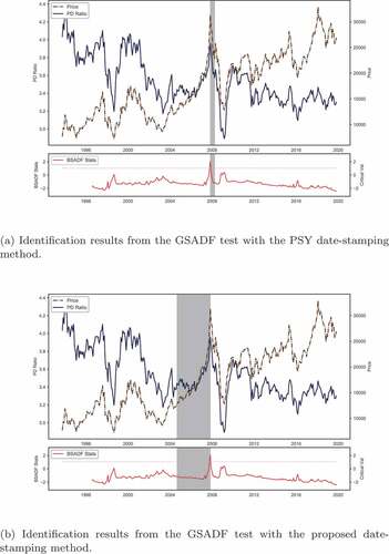
To illustrate the differences between the two date-stamping methods, we used the Hong Kong stock market as an example. The PSY approach identified a five-month bubble from November 2007 to March 2018; this is illustrated in Figure 1, with the bubble period highlighted in grey. In contrast, the bubble period identified by the modified method was from April 2004 to October 2007 as shown in Figure 1b. Unlike the PSY approach, the result of the modified method did not indicate shorter durations and agreed well with the asset price bubble cycles of the subprime mortgage crisis (see Dell’ariccia, Igan, & Laeven, 2012; Lewis, 2009; Tridico, 2012).

Figure 1. Bubble identification results for the hong kong stock market.

5.2. Backtesting results

We defined the pre-bubble and post-burst periods as 2 years before and after the bubble.

(14) $\mathrm{pre}-\mathrm{bubble}\mathrm{period}:\left[⌊\mathit{T}{\bar{r}}_{\mathit{e}}⌋-\mathit{p},⌊\mathit{T}{\bar{r}}_{\mathit{e}}⌋\right]$(14)

(15) $\mathrm{post}-\mathrm{burst}\mathrm{period}:\left[⌊\mathit{T}{\bar{r}}_{\mathit{f}}⌋,⌊\mathit{T}{\bar{r}}_{\mathit{f}}+\mathit{p}⌋\right]$(15)

Here $\mathit{p}$ is the time frequency-dependent parameter; $\mathit{p}=24$ for the monthly data and $\mathit{p}=500$ for the daily data (we assume 250 trading days per year). The pre-bubble period extended from September 2002 to August 2004 and the post-burst period from November 2007 to October 2009 for a bubble period identified from September 2004 to October 2007, when Hong Kong was used as an example. Further, we define the period not covered by the pre-bubble, bubble, and post-burst periods as ”normal periods.” For example, two normal periods of September 1993 to August 2002 and November 2009 to October 2019 were defined from the entire period considered for the Hong Kong market (September 1993 to October 2019). Table 5 shows the bubble periods identified for the nine stock markets. One bubble period was identified each for Australia, Canada, China, Germany, Hong Kong, Japan, and the UK, and two each for Spain and the US. The reason for the additional bubble period in Spain and the US could be the extent of data available. Spain’s data starts from January 1991 and the US’s data from February 1978.

Table 5. Full, pre-bubble, bubble, post-burst, and normal periods for the bubbles examined in the nine stock markets

		Country/Region
	Periods	AU	CA	CN	DE	ES	HK	JP	UK	US
Full		2000M4	1993M5	1997M11	1997M5	1991M1	1993M9	1993M5	2002 M2	1978 M2
		to	to	to	to	to	to	to	to	to
		2019M10	2019M10	2019M10	2019M10	2019M10	2019M10	2019M10	2019M10	2019M10
Pre-bubble	Period 1	2001M5	2000M11	2002M08	2003M5	1992 M2	2002M9	2001M6	2002M4	1987M8
		to	to	to	to	to	to	to	to	to
		2003M4	2002M10	2004M7	2005M4	1994M1	2004M8	2003M5	2004 M3	1989M7
	Period 2					2002M10				2002M4
						to				to
						2004M7*				2003 M2*
Bubble	Period 1	2003M5	2002M11	2004M8	2005M5	1994 M2	2004M9	2003M6	2004M4	1989M8
		to	to	to	to	to	to	to	to	to
		2009 M2	2009 M2	2007M5	2009 M3	2000M9	2007M10	2009 M2	2009 M2	2000 M3
	Period 2					2004M8				2003 M3
						to				to
						2009M5				2009 M3
Post-burst	Period 1	2009 M3	2009 M3	2007M6	2009M4	2000M10	2007M11	2009 M3	2009 M3	2000M4
		to	to	to	to	to	to	to	to	to
		2011 M2	2011 M2	2009M5	2011 M3	2002M9	2009M10	2011 M2	2011 M2	2002 M3
	Period 2					2009M6				2009M4
						to				to
						2011M5				2011 M3
Normal	Period 1	2000M4	1993M5	1997M11	1997M5	1991M1	1993M9	1993M5	2002 M2	1978 M2
		to	to	to	to	to	to	to	to	to
		2001M4	2000M10	2002M7	2003M4	1992M1	2002M8	2001M5	2002 M3	1987M7
	Period 2	2011 M3	2011 M3	2009M6	2011M4	2011M6	2009M11	2011 M3	2011 M3	2011M4
		to	to	to	to	to	to	to	to	to
		2019M10	2019M10	2019M10	2019M10	2019M10	2019M10	2019M10	2019M10	2019M10

^*As the duration between the bubble period is less than four years (two years for the first bubble’s post-burst period and two years for the second bubble’s pre-bubble period), the duration of the pre-bubble period of the second bubble is less than two years.

Tables 6 and 7 show the results of the RiskMetrics VaR backtests, and Tables 8 and 9 show the results of RiskMetrics 2006 in different periods. In all the hypothesis tests, we tested the null hypotheses at a significance level of 5%. For the periods where no VaR violation was observed, we have not reported the value for the independence tests as the results of the violation clustering test were ambiguous (see an example of the independence test and joint test results in the normal period for the UK (period 1) in Table 7). In the coverage tests, to deem a case as a ”failure,” the null hypotheses should be rejected in both coverage tests. An analogous criterion was also adopted for the independence tests and joint tests.

Table 6. Backtest results of riskmetrics VaR in the pre-bubble, bubble, and post-burst periods

			Tests
			Coverage Test		Independence Test		Joint Test
Period	Country/Region	Violations/nobs	POF	TUFF	Christoffersen	Mixed-Kupiec	Christoffersen	Mixed-Kupiec
	AU	6/507	0.687	0.968	0.704	0.220	0.858	0.297
	CA	7/503	0.405	0.783	0.002*	0.003*	0.006*	0.004*
	CN	2/482	0.144	0.500	0.897	0.337	0.341	0.229
	DE	2/510	0.116	0.028*	0.003*	0.001*	0.003*	0.001*
Pre-bubble	ES (Period 1)	9/504	0.110	0.871	0.144	0.000*	0.096	0.000*
	ES (Period 2)	2/458	0.173	0.102	0.895	0.185	0.391	0.155
	HK	6/496	0.650	0.205	0.701	0.125	0.838	0.178
	JP	3/492	0.348	0.764	0.848	0.039*	0.633	0.055
	UK	13/507 [12/507]	0.003* [0.009*]	0.542	0.038* [0.028*]	0.000*	0.002* [0.020*]	0.000*
	US (Period 1)	9/505	0.112	0.489	0.000*	0.000*	0.000*	0.000*
	US (Period 2)	5/232	0.125	0.745	0.083	0.004*	0.068	0.003*
	AU	43/1,478	0.000*	0.268	0.041*	0.000*	0.000*	0.000*
	CA	55/1,592 [54/1,592]	0.000*	0.992	0.001* [0.002*]	0.000*	0.000*	0.000*
	CN	17/684	0.001*	0.521	0.352	0.001*	0.003*	0.000*
	DE	33/998	0.000*	0.521	0.926	0.000*	0.000*	0.000*
Bubble	ES (Period 1)	39/1,675	0.000*	0.002*	0.002*	0.000*	0.000*	0.000*
	ES (Period 2)	33/1,223	0.000*	0.038*	0.176	0.000*	0.000*	0.000*
	HK	24/783	0.000*	0.307	0.763	0.000*	0.000*	0.000*
	JP	46/1,412	0.000*	0.820	0.261	0.000*	0.000*	0.000*
	UK	43/1,242 [42/1,242]	0.000*	0.255	0.074 [0.228]	0.000*	0.000*	0.000*
	US (Period 1)	53/2,697	0.000*	0.563	0.108	0.000*	0.000*	0.000*
	US (Period 2)	45/1,532	0.000*	0.102	0.193	0.000*	0.000*	0.000*
	AU	3/506	0.319	0.168	0.850	0.031*	0.598	0.042*
	CA	1/501	0.028*	0.130	0.950	0.130	0.089	0.028*
	CN	14/488	0.001*	0.011*	0.410	0.000*	0.002*	0.000*
	DE	4/511	0.608	0.215	0.801	0.125	0.849	0.187
Post-burst	ES (Period 1)	13/499	0.003*	0.068	0.404	0.001*	0.008*	0.000*
	ES (Period 2)	6/512	0.704	0.536	0.706	0.016*	0.866	0.028*
	HK	17/492	0.000*	0.011*	0.017*	0.000*	0.000*	0.000*
	JP	5/488	0.957	0.200	0.035*	0.005*	0.109	0.010*
	UK	6/505	0.680	0.191	0.704	0.001*	0.854	0.002*
	US (Period 1)	4/497	0.651	0.089	0.799	0.212	0.874	0.302
	US (Period 2)	6/505	0.680	0.219	0.704	0.035*	0.854	0.056

The backtest results of the RiskMetrics models that based on t-distribution do not differ from those with normal distribution. The only different results from t-distribution are shown in the square bracket[].

The decimal numbers in the cells are the p-values for assessing the null hypothesis that the model adequately measures the downside risk. Asterisk (*) indicates a p-value of less than 0.05.

Table 7. Backtest results of riskmetrics VaR in the normal and full periods

			Tests
			Coverage Test		Independence Test		Joint Test
Period	Country/Region	Violations/nobs	POF	TUFF	Christoffersen	Mixed-Kupiec	Christoffersen	Mixed-Kupiec
	AU (Period 1)	1/270	0.233	0.100	0.931	0.100	0.489	0.127
	AU (Period 2)	47/2,196	0.000*	0.686	0.000*	0.000*	0.000*	0.000*
	CA (Period 1)	51/1,888	0.000*	0.499	0.216	0.000*	0.000*	0.000*
	CA (Period 2)	58/2,177 [57/2,177]	0.000*	0.068	0.000*	0.000*	0.000*	0.000*
	CN (Period 1)	24/1,141	0.001*	0.459	0.100	0.000*	0.001*	0.000*
	CN (Period 2)	55/2,536	0.000*	0.595	0.007*	0.000*	0.000*	0.000*
	DE (Period 1)	37/1,513	0.000*	0.176	0.012*	0.000*	0.000*	0.000*
	DE (Period 2)	53/2,175	0.000*	0.735	0.000*	0.000*	0.000*	0.000*
	ES (Period 1)	2/269	0.658	0.624	0.862	0.884	0.893	0.931
Normal	ES (Period 2)	35/2,155	0.008*	0.467	0.282	0.000*	0.016*	0.000*
	HK (Period 1)	40/2,222	0.001*	0.909	0.000*	0.000*	0.000*	0.000*
	HK (Period 2)	53/2,465	0.000*	0.199	0.891	0.000*	0.000*	0.000*
	JP (Period 1)	37/1,992	0.001*	0.789	0.187	0.000*	0.001*	0.000*
	JP (Period 2)	45/2,125	0.000*	0.089	0.016*	0.000*	0.000*	0.000*
	UK (Period 1)	0/40	0.370	0.423	N/A	N/A	N/A	N/A
	UK (Period 2)	46/2,192	0.000*	0.945	0.000*	0.000*	0.000*	0.000*
	US (Period 1)	33/2,402	0.081	0.070	0.477	0.000*	0.170	0.000*
	US (Period 2)	57/2,161	0.000*	0.455	0.004*	0.000*	0.000*	0.000*
	AU	100/4,957	0.000*	0.100	0.000*	0.000*	0.000*	0.000*
	CA	172/6,661 [170/6,661]	0.000*	0.499	0.000*	0.000*	0.000*	0.000*
	CN	112/5,331	0.000*	0.459	0.003*	0.000*	0.000*	0.000*
	DE	129/5,707	0.000*	0.176	0.000*	0.000*	0.000*	0.000*
Full	ES	139/7,295	0.000*	0.624	0.070	0.000*	0.000*	0.000*
	HK	140/6,458	0.000*	0.909	0.000*	0.000*	0.000*	0.000*
	JP	136/6,509	0.000*	0.789	0.001*	0.000*	0.000*	0.000*
	UK	108/4,486 [106/4,486]	0.000*	0.926	0.000*	0.000*	0.000*	0.000*
	US	212/10,531	0.000*	0.070	0.000*	0.000*	0.000*	0.000*

The backtest results of the RiskMetrics models that based on t-distribution do not differ from those with normal distribution. The only different results from t-distribution are shown in the square bracket[].

The decimal numbers in the cells are the p-values for assessing the null hypothesis that the model adequately measures the downside risk. Asterisk (*) indicates a p-value of less than 0.05.

Table 8. Backtest Results of RiskMetrics 2006 VaR in the Pre-bubble, Bubble, and Post-burst Periods

			Tests
			Coverage Test		Independence Test		Joint Test
Period	Country/Region	Violations/nobs	POF	TUFF	Christoffersen	Mixed-Kupiec	Christoffersen	Mixed-Kupiec
	AU	4/507	0.620	0.968	0.801	0.179	0.857	0.258
	CA	2/503	0.122	0.783	0.899	0.898	0.300	0.457
	CN	0/482	0.002*	0.033*	N/A	N/A	N/A	N/A
	DE	1/510	0.026*	0.362	0.950	0.362	0.083	0.055
Pre-bubble	ES (Period 1)	1/504	0.027*	0.070	0.950	0.070	0.087	0.017*
	ES (Period 2)	1/458	0.042*	0.102	0.947	0.102	0.126	0.033*
	HK	3/496	0.340	0.205	0.848	0.327	0.623	0.359
	JP	1/492	0.030*	0.764	0.949	0.764	0.096	0.092
	UK	2/507	0.118	0.304	0.900	0.321	0.293	0.195
	US (Period 1)	5/505	0.982	0.489	0.034*	0.020*	0.105	0.037*
	US (Period 2)	0/232	0.031*	0.326	N/A	N/A	N/A	N/A
	AU	11/1,478	0.301	0.268	0.685	0.190	0.589	0.196
	CA	13/1,592	0.447	0.992	0.644	0.507	0.673	0.539
	CN	5/684	0.458	0.047*	0.786	0.187	0.732	0.236
	DE	5/998	0.080	0.235	0.820	0.719	0.210	0.429
Bubble	ES (Period 1)	10/1,675	0.073	0.338	0.729	0.674	0.189	0.465
	ES (Period 2)	13/1,223	0.827	0.536	0.597	0.197	0.849	0.251
	HK	5/783	0.276	0.307	0.800	0.878	0.535	0.813
	JP	15/1,412	0.816	0.820	0.570	0.060	0.828	0.082
	UK	11/1,242	0.680	0.077	0.657	0.010*	0.832	0.015*
	US (Period 1)	25/2,697	0.700	0.563	0.494	0.172	0.735	0.204
	US (Period 2)	6/1,532	0.006*	0.003*	0.828	0.029*	0.024*	0.003*
	AU	0/506	0.001*	0.027*	N/A	N/A	N/A	N/A
	CA	0/501	0.002*	0.028*	N/A	N/A	N/A	N/A
	CN	5/488	0.957	0.011*	0.035*	0.001*	0.109	0.002*
	DE	1/510	0.026*	0.029*	0.950	0.029*	0.082	0.008*
Post-burst	ES (Period 1)	2/499	0.126	0.531	0.899	0.749	0.308	0.404
	ES (Period 2)	3/512	0.307	0.536	0.851	0.175	0.584	0.200
	HK	4/492	0.667	0.553	0.798	0.096	0.882	0.153
	JP	0/488	0.002*	0.032*	N/A	N/A	N/A	N/A
	UK	0/505	0.001*	0.027*	N/A	N/A	N/A	N/A
	US (Period 1)	4/497	0.651	0.089	0.799	0.424	0.834	0.539
	US (Period 2)	0/505	0.001*	0.027*	N/A	N/A	N/A	N/A

The decimal numbers in the cells are the p-values for assessing the null hypothesis that the model adequately measures the downside risk. Asterisk (*) indicates a p-value of less than 0.05.

Table 9. Backtest results of riskmetrics 2006 VaR in the full and normal periods

			Tests
			Coverage Test		Independence Test		Joint Test
Period	Country/Region	Violations/nobs	POF	TUFF	Christoffersen	Mixed-Kupiec	Christoffersen	Mixed-Kupiec
	AU (Period 1)	2/270	0.654	0.100	0.863	0.258	0.891	0.405
	AU (Period 2)	18/2,196	0.381	0.923	0.008*	0.004*	0.019*	0.005*
	CA (Period 1)	20/1,888	0.798	0.499	0.513	0.892	0.781	0.919
	CA (Period 2)	22/2,177	0.961	0.930	0.503	0.078	0.798	0.100
	CN (Period 1)	7/1,141	0.158	0.532	0.769	0.682	0.353	0.557
	CN (Period 2)	32/2,536	0.203	0.456	0.366	0.006*	0.295	0.006*
	DE (Period 1)	5/1,513	0.002*	0.810	0.856	0.006*	0.010*	0.000*
	DE (Period 2)	11/2,175	0.011*	0.917	0.738	0.112	0.036*	0.024*
	ES (Period 1)	2/269	0.658	0.624	0.862	0.884	0.893	0.931
Normal	ES (Period 2)	13/2,155	0.046*	0.542	0.691	0.468	0.126	0.271
	HK (Period 1)	16/2,222	0.163	0.909	0.103	0.009*	0.100	0.008*
	HK (Period 2)	15/2,465	0.035*	0.199	0.668	0.146	0.099	0.067
	JP (Period 1)	9/1,992	0.006*	0.517	0.775	0.029*	0.022*	0.004*
	JP (Period 2)	18/2,125	0.467	0.089	0.008*	0.008*	0.023*	0.010*
	UK (Period 1)	0/40	0.370	0.423	N/A	N/A	N/A	N/A
	UK (Period 2)	12/2,192	0.020*	0.938	0.054	0.027*	0.010*	0.008*
	US (Period 1)	12/2,402	0.006*	0.070	0.728	0.047*	0.023*	0.007*
	US (Period 2)	25/2,161	0.475	0.445	0.002*	0.000*	0.008*	0.000*
	AU	34/4,957	0.028*	0.100	0.025*	0.000*	0.007*	0.000*
	CA	57/6,661	0.225	0.499	0.321	0.141	0.293	0.135
	CN	49/5,331	0.548	0.532	0.476	0.000*	0.647	0.000*
	DE	23/5,707	0.000*	0.810	0.666	0.000*	0.000*	0.000*
Full	ES	45/7,295	0.000*	0.624	0.455	0.048*	0.001*	0.005*
	HK	43/6,458	0.004*	0.909	0.296	0.006*	0.009*	0.001*
	JP	43/6,509	0.003*	0.517	0.034*	0.000*	0.001*	0.000*
	UK	25/4,486	0.001*	0.213	0.131	0.000*	0.002*	0.000*
	US	77/10,531	0.004*	0.070	0.003*	0.000*	0.000*	0.000*

The decimal numbers in the cells are the p-values for assessing the null hypothesis that the model adequately measures the downside risk. Asterisk (*) indicates a p-value of less than 0.05.

Table 6 shows that RiskMetrics performed poorly around turbulent financial times. Both the RiskMetrics models with normal distribution and $\mathit{t}$-distribution had analogous results. Minor differences were found in Canada and the UK but such have no impact on the results in the hypothesis tests. Within the large estimation window size used in the RiskMetrics model the fitted $\mathit{t}$-distribution approaches the normal. Further, RiskMetrics performed effectively only in the coverage tests for the pre-bubble period. We could not reject the null hypothesis because the probability of a violation was the same as the coverage rate for Australia, Canada, China, Spain, Hong Kong, Japan, and the US markets. The exceptions were Germany (p-value was 0.028 in the TUFF test) and the UK markets (p-value was 0.003 in the POF test). Violation clustering was also noted with Canada, Germany, the UK, and the US, which led to rejecting the null hypotheses in these markets in all the joint tests.

RiskMetrics performed inadequately in the bubble period as well. The null hypotheses of the POF coverage tests were rejected in all the nine markets. Although the Christoffersen’s independence test showed no significant consecutive violations, the violation clustering was severe leading to the null hypotheses being rejected by the mixed-Kupiec independence test and all the joint tests. However, RiskMetrics performed noticeably better in the post-burst period as it rejected the null hypotheses only for China, Hong Kong, and Japan. The coverage tests (with a p-value of 0.001 in the POF test, and 0.011 in the TUFF test) showed that the number of violations in China was misspecified. The independence tests showed that the Japanese market exhibited violation clusters (with a p-value of 0.035 in the Christoffersen test and 0.005 in the mixed-Kupiec test). In the post-burst period, RiskMetrics underestimated the downside risk in China, Hong Kong, and Japan. Further, Table 7 shows that RiskMetrics presented inaccurate downside risk measures for both the normal and full periods. Similar to the results for the bubble period, the null hypotheses were rejected in most of the POF coverage tests, independence tests, and joint tests. We found that RiskMetrics failed to reveal the downside risk in most cases.

The results in Table 8 provide convincing evidence to show that RiskMetrics 2006 works efficiently in a period of market turbulence. In the pre-bubble period, we could not reject the null hypotheses in all the tests, except for China and the US. In China, the null hypothesis was rejected by both coverage tests (the p-value was 0.002 in the POF test and 0.033 in the TUFF test). In the US, both the independence tests (period 1) rejected the null hypothesis (with p-values of 0.034 and 0.020). Further, RiskMetrics 2006 performed efficiently in the bubble period. It failed only in the coverage tests and joint tests for the US market in period 2, defined in Table 5. However, the long memory RiskMetrics 2006 behaved conservatively in the post-burst period although no violation was found in Australia, Canada, Japan, the UK, and the US (period 2). In the normal period, RiskMetrics 2006 performed efficiently; failing only in period 2 of the independence tests for Australia (with a p-value of 0.008 in the Christoffersen test and 0.004 in the mixed-Kupiec test), Japan (with a p-value of 0.008 in the Christoffersen test and 0.008 in the mixed-Kupiec test), and the US (with a p-value of 0.002 in the Christoffersen test and 0.000 in the mixed-Kupiec test).

RiskMetrics 2006 behaved conservatively in overestimating the downside risk after the bubbles. However, in the total duration considered, the number of VaR violations were 34, 57, 49, 23, 45, 43, 43, 25, and 77 in Australia, Canada, China, Spain, Hong Kong, Japan, the UK, and the US, respectively. These violation numbers were significantly lower than those found by the RiskMetrics model, which were 100, 172, 112, 129, 139, 140, 146, 108, and 212, respectively, as shown in Table 7. Although RiskMetrics 2006 may require financial institutions to allocate more capital than necessary to manage risks, it performed efficiently in most periods.

5.3. VaR performance in pre-bubble, bubble, and post-burst periods

We conducted the Fisher’s exact tests for both the RiskMetrics and RiskMetrics 2006 models to gain further insight on their performance in different crisis periods. We performed 10 Fisher’s exact tests to compare the VaR performance in each of the nine markets during the full, pre-bubble, bubble, post-burst, and normal periods. The results are shown in Table 10. Table 10 shows that unlike RiskMetrics, the RiskMetrics 2006 has a consistent performance regardless of the periods in all the nine markets. In each panel, the lower triangular matrix contain the p-values of the RiskMetrics tests, while the upper triangular matrix contains the p-values of the RiskMetrics 2006 tests. A p-value of Fisher test greater than 5% is indicative of no statistically significant relationship of the VaR failure rates between two chosen periods. Panels 10(a), 10(g), and 10(h) show that the performance of RiskMetrics VaR differed in the bubble periods. The null hypotheses were rejected in the tests between the bubble period and the pre-bubble, post-burst, and full periods. After combining the results in Tables 6 and 7, the performance of RiskMetrics was found to be inconsistent in different periods, with the frequency of failure being higher in the bubble periods. Panel 10(i) shows considerable difference with RiskMetrics in the US post-burst period when compared to other periods. Comparing this with the results in Table 6, we observe that the RiskMetrics model failed in all the periods in the US except for the post-burst period. Similarly, panel 10(c) shows that it only performed well in the pre-bubble period in China. The overall results suggested a significant difference in the RiskMetrics performance across different countries in different crisis periods.

Table 10. Fisher exact test for the significance level of the difference of VaR failure rate by time period

Period	Pre-bubble	Bubble	Post-burst	Normal	Full	Pre-bubble	Bubble	Post-burst	Normal	Full
Pre-bubble		1.000	0.124	1.000	0.776		0.544	0.500	0.226	0.438
Bubble	0.031*		0.076	1.000	0.859	0.015*		0.047*	0.547	1.000
Post-burst	0.506	0.002*		0.036*	0.070	0.069	0.000*		0.012*	0.032*
Normal	0.278	0.062	0.036*		0.563	0.097	0.134	0.000*		0.351
Full	0.237	0.044*	0.024*	0.861		0.104	0.060	0.000*	0.756
	(a) Australia					(b) Canada
Period	Pre-bubble	Bubble	Post-burst	Normal	Full	Pre-bubble	Bubble	Post-burst	Normal	Full
Pre-bubble		0.081	0.062	0.019*	0.032*		0.670	1.000	0.712	0.717
Bubble	0.005*		0.750	0.535	0.829	0.000*		0.670	0.790	0.597
Post-burst	0.004*	0.715		1.000	0.803	0.687	0.002*		0.712	0.717
Normal	0.005*	0.570	0.326		0.515	0.001*	0.146	0.015*		0.870
Full	0.005*	0.484	0.255	0.882		0.002*	0.057	0.024*	0.576
	(c) China					(d) Germany
Period	Pre-bubble	Bubble	Post-burst	Normal	Full	Pre-bubble	Bubble	Post-burst	Normal	Full
Pre-bubble		0.061	0.453	0.178	0.166		1.000	0.725	1.000	1.000
Bubble	0.014*		0.394	0.515	0.345	0.037*		0.740	1.000	1.000
Post-burst	0.201	0.332		0.808	0.828	0.021*	0.745		0.570	0.573
Normal	0.519	0.015*	0.462		1.000	0.300	0.061	0.046*		1.000
Full	0.122	0.076	1.000	0.253		0.192	0.125	0.081	0.546
	(e) Spain					(f) Hong Kong
Period	Pre-bubble	Bubble	Post-burst	Normal	Full	Pre-bubble	Bubble	Post-burst	Normal	Full
Pre-bubble		0.087	1.000	0.356	0.368		0.369	0.500	1.000	1.000
Bubble	0.001*		0.016*	0.154	0.120	0.372		0.040*	0.275	0.221
Post-burst	0.504	0.008*		0.107	0.072	0.163	0.010*		0.139	0.170
Normal	0.031	0.010*	0.160		1.000	0.497	0.014*	0.277		1.000
Full	0.018*	0.011*	0.131	0.779		0.762	0.045*	0.085	0.388
	(g) Japan					(h) United Kingdom
Period	Pre-bubble	Bubble	Post-burst	Normal	Full
Pre-bubble		1.000	0.507	0.796	1.000
Bubble	0.590		0.289	0.432	1.000
Post-burst	0.145	0.006*		0.639	0.320
Normal	1.000	0.269	0.035*		0.392
Full	1.000	0.253	0.022*	0.899
			(i) United States

The decimal numbers in the cells are the p-values for assessing the null hypothesis that the VaR failure rates show no significant differences between the periods. The results of RiskMetrics are shown in the lower triangular matrix (non-shaded) and the results of RiskMetrics 2006 are shown in the upper triangular matrix (shaded). Asterisk (*) indicates a p-value of less than 0.05. P-value of Fisher test larger than 0.05 is indicative no statistically significant relationship of the VaR failure between two chosen periods.

Contrary to RiskMetrics, RiskMetrics 2006 did not show extensive performance differences in different periods. The VaR performance seen panel 10(d), panel 10(e), panel 10(f), panel 10(i) shows no significant difference, whereas occasional inconsistencies are observed in panel 10(b), 10(g), and 10(h). Specifically, the inconsistency in these three panels was between the bubble and the post-burst periods. The Fisher’s test results support our finding previously mentioned in section 5.2 that though RiskMetrics 2006 occasionally overstated the downside risk in post-burst periods, it performed efficiently in most periods.

6. Summary and conclusions

In this study, we conducted empirical tests to respond to the criticism that VaR models fail during financial crises when asset bubbles burst. Our empirical tests on the nine markets, namely Australia, Canada, China, Spain, Hong Kong, Japan, the UK, and the US, were conducted using data from the earliest available dates to October 2019. Asset price bubbles were date-stamped using the modified PSY tests on the log price-dividend ratios of these nine markets. However, as the date-stamping method of the original PSY test is forward-looking, it selects the ending point of the testing window as the bubble origination date. To suit our need for a backward-looking date-stamping method for the backtests, we modified the date-stamping method by choosing the starting point of the testing window. Our results show that the original date-stamping method has time lag and indicates a shorter duration for the bubble period. It date-stamps the bubble start near the end of a true bubble and the average duration of the bubble periods detected is 8 months. The results also show that our modified method addressed both the time lag and shorter duration issues present in the original date-stamping method and, thus, more suitable for backtesting.

The empirical test results of the nine backtests allowed us to draw two main conclusions. First, the RiskMetrics 2006 model outperforms the RiskMetrics model. Specifically, the former works well in pre-bubble, bubble, and normal periods but behaves conservatively in the post-burst period, which may overestimate the downside risk. Second, the criticism that all VaR models fail in crisis or bubble periods is statistically invalid. The power of VaR is affected by the modelling practices adopted by different financial institutions.

An interesting direction for future research would be to examine parametric and non-parametric VaR approaches. Non-parametric approaches comprise historical and Monte Carlo simulations, whereas parametric approaches include GARCH, GJR-GARCH (Glosten, Jagannathan, & Runkle, 1993), and the multivariate DCC (Engle, 2002) approach.

Disclosure statement

No potential conflict of interest was reported by the author(s).

Additional information

Notes on contributors

Raymond Kwong

Raymond Kwong is a Senior Lecturer in the College of Professional and Continuing Education, the Hong Kong Polytechnic University. He received his PhD in Economics from the Newcastle University, United Kingdom. His research focuses on issues of asset price bubbles, market microstructure, price discovery and risk management in equity market.

Helen Wong

Helen Wong is a Principal Lecturer in the College of Professional and Continuing Education, the Hong Kong Polytechnic University (HKPU). She has devoted her research study in customer relationship building, corporate social responsibility, accounting and finance. Prior joining HKPU, Helen has worked in several renowned corporations in Hong Kong and Canada, such as PricewaterhouseCoopers, Hong Kong Stock Exchange, University of Toronto, and Bank of Montreal.

Appendix A.

Technical details of VaR backtests

A.1. Unconditional Coverage Tests

The POF test examines whether the observed fail rate (number of VaR violations) is significantly different from the selected failure rate $\mathit{p}$. The null hypothesis of the POF test is $H_0:\mathit{p}=\hat{p}={\nu }_1/W_T$, and equation A.1 defines the likelihood ratio test statistic of the POF test. Under the null hypothesis, the likelihood ratio test statistic $\mathit{L}{R}_{\mathit{POF}}$ is asymptotically ${\chi }^2$-distributed with 1 degree of freedom.

The TUFF test assesses the time it takes for the first violation to occur. It assumes that the first violation occurs in $\mathit{\nu }=1/\mathit{p}$ days. For the 1% VaR calculation, a violation is expected to occur every 100 days. The null hypothesis of the TUFF test is $H_0:\mathit{p}=\hat{p}=1/\mathit{\nu }$. Equation A.2 defines the likelihood ratio test statistic of the TUFF test. Similar to the POF test, under the null hypothesis, the likelihood ratio test statistic $\mathit{L}{R}_{\mathit{TUFF}}$ is asymptotically ${\chi }^2$-distributed with 1 degree of freedom.

(A.1) $\mathit{L}{R}_{\mathit{POF}}=-2\mathit{ln}\left(\frac{{(1-\mathit{p})}^{W_T-{\nu }_1}{p}^{{\nu }_1}}{{(1-\hat{p})}^{W_T-{\nu }_1}{\hat{p}}^{{\nu }_1}}\right)$(A.1)

(A.2) $\mathit{L}{R}_{\mathit{TUFF}}=-2\mathit{ln}\left(\frac{\mathit{p}{(1-\mathit{p})}^{\mathit{\nu }-1}}{\hat{p}{(1-\hat{p})}^{\mathit{\nu }-1}}\right)$(A.2)

A.2. Conditional Coverage Tests

Christoffersen’s independence test uses a binary first-order Markov chain and a transition probability matrix $\mathrm{\Pi }$ to test the independence of the violations.

(A.3) ${\mathrm{\Pi }}_1=\left(\begin{array}{cc}(1-p_{01})& p_{01}\\ (1-p_{11})& p_{11}\end{array}\right)$(A.3)

Indicator variable $I_t$ takes the value 1 when a VaR violation occurs and 0 otherwise, and $p_{\mathit{ij}}=\mathit{Pr}(I_t=\mathit{j}|I_{\mathit{t}-1}=\mathit{i})$. Christoffersen and Pelletier (2004) suggested that the likelihood function for the violation sequence is Bernoulli-distributed and follows the first-order Markov chain of equation A.4.

(A.4) $L_U({\mathrm{\Pi }}_1;I_1,I_2,\cdots ,I_t)=(1-p_{01}{)}^{{\mathit{n}}_{00}}{p}_{01}^{{\mathit{n}}_{01}}(1-p_{11}{)}^{{\mathit{n}}_{10}}{p}_{11}^{{\mathit{n}}_{11}}$(A.4)

where $n_{\mathit{ij}}$ is the total number of observations occurring after $I_{\mathit{t}-1}=\mathit{i}$, until $I_t=\mathit{j}$. The unrestricted form of the maximum likelihood estimates for the log-likelihood functions $L_U({\mathrm{\Pi }}_1)$ are simply ratios of the counts of the respective cells as shown in equation A.5.

(A.5) ${\mathrm{\Pi }}_1=\left(\begin{array}{cc}\frac{{\mathit{n}}_{00}}{n_{00}+n_{01}}& \frac{{\mathit{n}}_{01}}{n_{00}+n_{01}}\\ \frac{{\mathit{n}}_{10}}{n_{10}+n_{11}}& \frac{{\mathit{n}}_{11}}{n_{00}+n_{11}}\end{array}\right)$(A.5)

If the violations are independent, the violation on day $\mathit{t}$ is independent from that on day $\mathit{t}-1$; thus, the probability $p_{01}$ should be equal to $p_{11}$. Equation A.6 shows the transition probability matrix under the null hypothesis $H_0:p_{01}=p_{11}=\hat{p}$ and equation A.7 shows the restricted form of the maximum likelihood estimates for the log-likelihood function $L_R({\mathrm{\Pi }}_0)$.

(A.6) $H_0:{\mathrm{\Pi }}_0=\left(\begin{array}{cc}(1-\hat{p})& \hat{p}\\ (1-\hat{p})& \hat{p}\end{array}\right)$(A.6)

(A.7) $L_R({\mathrm{\Pi }}_0|;I_1,I_2,\cdots ,I_t)=(1-\hat{p}{)}^{{\mathit{n}}_{00}+n_{10}}{\hat{p}}^{n_{01}+n_{11}}$(A.7)

where $\hat{p}=(n_{01}+n_{11})/(n_{00}+n_{01}+n_{10}+n_{11})$. Equation A.8 shows the likelihood ratio test statistic for independence, $\mathit{L}{R}_{in{d}_c}$, which is asymptotically ${\chi }^2$-distributed with 1 degree of freedom under the null hypothesis of the restricted model being the preferred model.

(A.8) $\mathit{L}{R}_{in{d}_c}=2(\mathit{log}{L}_U({\mathrm{\Pi }}_0)-\mathit{log}{L}_R({\mathrm{\Pi }}_1))\sim {\chi }^2(1)$(A.8)

Hass (2001) proposed the mixed-Kupiec independence test, which combined the ideas of Christoffersen and Kupiec, to consider the timing of different occurrences to test the independence of the violations. The mixed-Kupiec test overcomes the limitation of Christoffersen’s independence test in which the first-order Markov chain considers only the dependence between two consecutive trading days. Equation A.9 shows the likelihood ratio statistic $\mathit{L}{R}_{\mathit{in}{\mathit{d}}_{\mathit{mk}}}$ of the mixed-Kupiec test.

(A.9) $\mathit{L}{R}_{\mathit{in}{\mathit{d}}_{\mathit{mk}}}=\sum _{\mathit{i}=1}^n-2\mathit{ln}\left(\frac{\mathit{p}{(1-\mathit{p})}^{b_i-1}}{(1/b_i)(1-1/b_i{)}^{b_i-1}}\right)$(A.9)

where $b_i$ is the time between VaR violations $\mathit{i}-1$ and $\mathit{i}$, and $\mathit{n}$ is the number of exceptions in the testing period.

A.3. Joint Coverage Tests

The joint test considers both the coverage and the independence of the violations by combining the likelihood ratios of both the tests. The Christoffersen joint test combines the likelihood ratios of the POF test and the Christoffersen’s independence test, whereas the mixed-Kupiec joint test combines the likelihood ratios of the TUFF test and the mixed-Kupiec independence test.

The Christoffersen joint test of coverage and independence can be performed by combining the $\mathit{L}{R}_{\mathit{POF}}$ and $\mathit{L}{R}_{in{d}_c}$ statistics. The null hypothesis is that there are no coverage and clustering issues. Under the null hypothesis, the conditional coverage $\mathit{L}{R}_{\mathit{CC}}$ statistic, shown in equation A.10, is asymptotically ${\chi }^2$-distributed with 2 degrees of freedom.

(A.10) $\mathit{L}{R}_{\mathit{cc}}=\mathit{L}{R}_{\mathit{POF}}+\mathit{L}{R}_{in{d}_c}\sim {\chi }^2(2)$(A.10)

Similarly, the mixed-Kupiec joint test combines the $\mathit{L}{R}_{\mathit{TUFF}}$ and $\mathit{L}{R}_{\mathit{in}{\mathit{d}}_{\mathit{mk}}}$ statistics into the conditional coverage $\mathit{L}{R}_{\mathit{mixed}}$ statistic. This statistic, shown in equation A.11, is asymptotically ${\chi }^2$-distributed with $(\mathit{n}+1)$ degrees of freedom under the null hypothesis.

(A.11) $\mathit{L}{R}_{\mathit{mixed}}=\mathit{L}{R}_{\mathit{TUFF}}+\mathit{L}{R}_{\mathit{in}{\mathit{d}}_{\mathit{mk}}}\sim {\chi }^2(\mathit{n}+1)$(A.11)

References

- Atkinson, T., Luttrell, D., & Rosenblum, H. (2013). Assessing the costs and consequences of the 2007–09 financial crisis and its aftermath. Economic Letter, 8(7). Retrieved from https://ideas.repec.org/a/fip/feddel/y2013isepnv.8no.7.html
- Bams, D., Blanchard, G., & Lehnert, T. (2017). Volatility measures and Value- at-Risk. International Journal of Forecasting, 33(4), 848–863. Retrieved from http://www.sciencedirect.com/science/article/pii/S0169207017300511
- Blanchard, O. J., & Watson, M. W. (1982, july). Bubbles, rational expectations and financial markets (Working Paper No. 945). National Bureau of Economic Research. Retrieved from http://www.nber.org/papers/w0945
- Bollerslev, T. (1986). Generalized autoregressive conditional heteroskedasticity. Journal of Econometrics, 31(3), 307–327. Retrieved from http://econpapers.repec.org/RePEc:eee:econom:v:31:y:1986:i:3:p:307-327
- Brown, M., Stein, S., & Zafar, B. (2015). The impact of housing markets on consumer debt: Credit report evidence from 1999 to 2012. Journal of Money, Credit and Banking, 47(S1), 175–213. Retrieved from https://onlinelibrary.wiley.com/doi/abs/10.1111/jmcb.12198
- Campbell, J. Y., & Shiller, R. J. (1989). The dividend-price ratio and expectations of future dividends and discount factors. The Review of Financial Studies, 1(3), 195–228.
- Chen, C. W. S., Gerlach, R., Lin, E. M. H., & Lee, W. C. W. (2012, December). Bayesian forecasting for financial risk management, pre and post the global financial crisis. Journal of Forecasting, 31(8), 661–687.
- Chiriac, R., & Voev, V. (2011, September). Modelling and forecasting multivariate realized volatility. Journal of Applied Econometrics, 26(6), 922–947.
- Christoffersen, P., & Pelletier, D. (2004). Backtesting value-at-risk: A duration- based approach. Journal of Financial Econometrics, 2(1), 84–108. Retrieved from http://jfec.oxfordjournals.org/content/2/1/84.abstract
- Dell’ariccia, G., Igan, D., & Laeven, L. (2012). Credit booms and lending standards: Evidence from the subprime mortgage market. Journal of Money, Credit and Banking, 44(2–3), 367–384. Retrieved from https://onlinelibrary.wiley.com/doi/abs/10.1111/j.1538-4616.2011.00491.x
- Demyanyk, Y., & Van Hemert, O. (2011). Understanding the subprime mortgage crisis. Review of Financial Studies, 24(6), 1848–1880.
- Dickey, D. A., & Fuller, W. A. (1979). Distribution of the estimators for autoregressive time series with a unit root. Journal of the American Statistical Association, 74(366a), 427–431.
- Engle, R. (2002). Dynamic conditional correlation. Journal of Business & Economic Statistics, 20(3), 339–350.
- Engle, R., Ledoit, O., & Wolf, M. (2019, April). Large dynamic covariance matrices. Journal of Business & Economic Statistics, 37(2), 363–375.
- Fisher, R. A. (1922, June). On the interpretation of χ2 from contingency tables, and the calculation of P. Journal of the Royal Statistical Society, 85(1), 87–94. Retrieved from http://www.jstor.org/stable/2340521
- Fiszeder, P., Fałdziński, M., & Molnár, P. (2019). Range-based DCC models for covariance and value-at-risk forecasting. Journal of Empirical Finance, 54, 58–76. Retrieved from http://www.sciencedirect.com/science/article/pii/S0927539819300696
- Glosten, L. R., Jagannathan, R., & Runkle, D. E. (1993, December). On the relation between the expected value and the volatility of the nominal excess return on stocks. The Journal of Finance, 48(5), 1779–1801.
- Halbleib, R., & Pohlmeier, W. (2012). Improving the value at risk forecasts: Theory and evidence from the financial crisis. Journal of Economic Dynamics and Control, 36(8), 1212–1228. Retrieved from http://www.sciencedirect.com/science/article/pii/S0165188912000887
- Hass, M. (2001). New methods in backtesting. Retrieved from www.ime.usp.br/rvicente/risco/haas.pdf
- Köksal, B., & Orhan, M. (2013). Market risk of developed and emerging countries during the global financial crisis. Emerging Markets Finance and Trade, 49(3), 20–34.
- Kupiec, P. H. (1995). Techniques for verifying the accuracy of risk measurement models. The Journal of Derivatives, 3(2), 85–93. Retrieved from http://ideas.repec.org/p/fip/fedgfe/95-24.html
- Law, K., Li, W. K., & Yu, P. (2020). An empirical evaluation of large dynamic covariance models in portfolio value-at-risk estimation. Journal of Risk Model Validation, 14(2), 21–39.
- Lee, M.-C., Chiou, J.-S., & Lin, C.-M. (2006, May). A study of value-at-risk on portfolio in stock return using DCC multivariate GARCH. Applied Financial Economics Letters, 2(3), 183–188.
- Lewis, M. K. (2009). The origins of the sub-prime crisis: Inappropriate policies, regulations, or both? Accounting Forum, 33(2), 114–126.
- Lockwood, E. (2015). Predicting the unpredictable: Value-at-risk, performativity, and the politics of financial uncertainty. Review of International Political Economy, 22(4), 719–756.
- Mertzanis, C. (2013). Risk management challenges after the financial crisis. Economic Notes, 42(3), 285–320. Retrieved from https://onlinelibrary.wiley.com/doi/abs/10.1111/j.1468-0300.2013.12011.x
- Mian, A., & Sufi, A. (2009). The consequences of mortgage credit expansion: Evidence from the U.S. mortgage default crisis*. The Quarterly Journal of Economics, 124(4), 1449–1496.
- Phillips, P., Shi, S., & Yu, J. (2014). Specification sensitivity in right-tailed unit root testing for explosive behaviour. Oxford Bulletin of Economics and Statistics, 76(3), 315–333. Retrieved from https://onlinelibrary.wiley.com/doi/abs/10.1111/obes.12026
- Phillips, P., Shi, S., & Yu, J. (2015). Testing for multiple bubbles: Historical episodes of exuberance and collapse in the S&P 500. International Economic Review, 56(4), 1043–1078.
- Phillips, P., Wu, Y., & Yu, J. (2011). Explosive behavior in the 1990S Nasdaq: When did exuberance escalate asset values?*. International Economic Review, 52(1), 201–226.
- Riskmetrics, T. M. (1996). JP morgan technical document. JP Morgan: New York.
- Sanders, A. (2008, December). The subprime crisis and its role in the financial crisis. Journal of Housing Economics, 17(4), 254–261. Retrieved from https://www.sciencedirect.com/science/article/pii/S1051137708000363
- Tridico, P. (2012). Financial crisis and global imbalances: Its labour market origins and the aftermath. Cambridge Journal of Economics, 36(1), 17–42.
- Zumbach, G. (2007). The riskmetrics 2006 methodology (Tech. Rep.). University of Applied Sciences Western Switzerland.