Money demand under a fixed exchange rate regime: the case of Saudi Arabia

ABSTRACT

This paper reviews earlier studies and shows that the money demand (MD) relationship under a fixed exchange rate (ER) regime differs from that under a floating ER regime, mainly due to the limited role of monetary policy in the former regime. It then empirically demonstrates that an open-economy model augmented with country-specific factors is a better framework for characterizing the MD function under a fixed ER regime by applying cointegration and equilibrium correction modeling to the Saudi data as a case study. The main message for monetary authorities is that there are other factors, besides those theoretically predicted, shaping MD under a fixed ER regime. This information is important for providing adequate money supply to support economic growth and maintain the stability of the fixed ER, as well as for checking the stability of the MD to make appropriate policy decisions.

KEYWORDS:

• money demand
• fixed exchange rate
• monetary policy
• oil price
• Saudi Arabia
• cointegration
• autometrics

1. Introduction

Monetary authorities require a correctly specified money demand (MD) function to design appropriate policies that boost economic growth and maintain macroeconomic stability. This function links money to other key macroeconomic indicators such as prices, output, interest rates and exchange rates (ERs). It is equally important for monetary authorities in countries with fixed ER regimes to maintain regime stability alongside the aforementioned targets. However, under fixed ER regimes, monetary policies (MPs) play a limited role as they are theoretically articulated (see e.g., Blomqvist, 1970; Mundell, 1960, 1962; Swoboda, 1973).¹ The Mundell–Fleming trilemma states that a country with a fixed ER and a free flow of capital loses its MP independence. The target of MP under a fixed ER regime is to keep the ER unchanged. Therefore, it cannot target inflation or output growth, nor can it use interest rates or money supply as instruments (e.g., Curtis & Irvine, 2021, ch. 12; Mankiw, 2003, ch. 12). This implies that the MD relationship under a fixed ER regime – and its implications for MP – should differ under a floating ER regime. However, this point has not drawn sufficient attention in the international MD literature.

To the best of our knowledge, no study has surveyed MD relationships in fixed and floating ER regimes to identify their main differences and specify a representative MD function through a combination of theory, empirical literature, and country-specific features. Further, no study has estimated such a function to determine the main implications for MP under a fixed ER regime. One consequence of this gap is that a number of studies, based on their findings regarding the stability of the MD function, have proposed recommendations (such as inflation targeting, monetary aggregate targeting or using interest rates as an instrument) that cannot be implemented under fixed ER regimes (e.g., Ali, 2017; Al-Qudah, 2019; Bhatta, 2011; Budha, 2011; Jayaraman & Ward, 2000; Mahmood & Asif, 2016; Mala, 2014). This is one of the motivations for the present study.

The second motivation is related to the stability of the MD relationship. Testing the stability of the MD function is crucial if monetary authorities plan to target a monetary aggregate or use it as an instrument (e.g., the discussions in Hossain, 2019). However, there are additional factors that necessitate this testing – for example, the effect of quantitative easing on long-term interest rates and its consequences for the MD relationship. In recent years, formulating a proper MD function and testing its stability has gained importance as economies face various changes caused by global economic developments. These include trade tensions, global accommodative MP, and volatile commodity prices (Hossain, 2019; Taylor, 2019). Another justification for stability testing is the implementation of structural and other reforms within economies.

With the aim of better understanding the MD relationship and its policy implications under a fixed ER regime, this study has four objectives: (i) to compare the main features of the MD relationship in fixed ER regimes to those of the relationship under floating ER regimes by reviewing the literature on both; (ii) to specify a function that better characterizes the MD relationship under a fixed ER regime through a combination of theory, a literature survey and country specificities; (iii) to estimate the function and test its stability and predictive ability; and (iv) to propose policy insights by underlining the limitations of MP under a fixed ER regime.

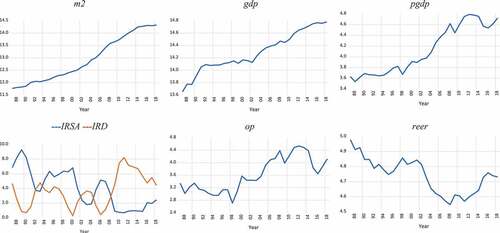
As a case study, we selected Saudi Arabia. It is a small, open, oil-rich economy with a fixed ER regime and free capital movement. Al-Jasser and Banafe (1999) discuss how MP is tied to ER policy in Saudi Arabia, with the objective of keeping the Unites States dollar/Saudi Arabian riyal (USD/SAR) ER as stable as possible in order to maintain economic confidence and encourage the inflow of foreign capital. Saudi Arabia has had a fixed ER policy since 1987, at 3.75 SAR/USD.² The country’s recent economic transformations (e.g., large-scale energy price and fiscal reforms) are unprecedented, and the oil price decreases were significant in 2015–2018 (Gonand, Hasanov, & Hunt, 2019; Hasanov, Joutz, Mikayilov, & Javid, 2020b). Further, the growth rates of the M2 broad monetary aggregate and GDP have slowed, with negative growth rates recorded for prices from 2013 to 2016 (see Figure 1). However, only five MD studies on Saudi Arabia cover the recent oil price drops and economic reforms implemented since 2016 (Table 1B); two of these neither conducted stability analyses nor checked the predictive abilities of their models.

Table 1. MD studies in economies with fixed ER regimes

Study	Country	Frequency	Money Measure	Explanatory variable	Unit Root Test	Cointegration Test	Stability Test	Estimated Long-run and SoA Coefficients
								Income	Interest Rate	ECTt-1
Marquez (1987)	Venezuela	1961–1980 A	M2N	NY, ER, IRD, IRF	NA	NA	NA	0.76**	NR	0.45**
Coppin (1991)	Barbados	1967–1987 A	M1	Y, M, X, IRD	NA	NA	NA	0.70**	−0.04**	NA
Darrat and Al-Mutawa (1996)	UAE	1974:1–1992:2 Q	M1	YN, INF, IRD, IRF, ER	DF, ADF	NA	C, FH; Yes	0.42**	−0.09	−0.40**
Jayaraman and Ward (2000)	Fiji Islands	1979:1–1996:4 Q	M2	Y, INF, REER, IRD	ADF	ADL	CU, CU^2; Yes	0.98	0.02**	−0.06**
Rother (1999)	West African Monetary Union	1975:1–1996:4 Q	M2	Y, IRD, INF, ID	ADF	JJ	NA	0.23**	0.63**	−0.21**
Nachega (2001)	Cameroon	1963–1993 A	M2	Y, INF, ER, IRD, IRF	ADF	JJ	NA	1.1**	7.7*	−0.6**
Katafono (2001)	Fiji Island	1975–1999 A	M1	Y, IRD, REER, SR	DF, PP	JJ	C; Yes	0.77**	0.006	−1.52**
Jayaraman and Ward (2000)	Fiji Island	1997:1–1996:4 Q	M2	Y, IRD, REER	ADF	ADL	C, CU^2; Yes	0.96	−0.04	−0.25
Bahmani-Oskooee and Ng (2002)	Hong Kong	1985:1–1999:4 Q	M2N	Y, IRD, IRF, NEER	NA	ADL	CU, CU^2; Yes	1.73**	−0.04**	−0.46**
Andersen (2004)	Denmark	1980:1–2002:4 Q	M2	Y, ER, ID	NA	NA	NA	0.84**	4.7*	NA
Harb (2004) ^P	Bahrain	1979–2000 A	M1	YN/C, IRD, ER	IPS, ADF, PP	P	NA	0.77**	−0.02	NR
	Kuwait							0.26	0.02	NR
	Oman							0.85**	−0.01	NR
	Qatar							−0.21	−0.02	NR
	UAE							1.00**	−0.02	NR
Hamori (2008) ^P	Sub-Saharan Africa	1980–2006 A	M2	Y, IRD	IPS, LLP, F-ADF	P, K, MW	NA	1.02**	−0.28**	NA
Lee, Chang, and Chen (2008) ^P	Bahrain	1979–2000 A	M1	Y, IRD, NER	NR	L	NA	0.63**	−0.09**	NR
	Kuwait							0.67**	0.08**	NR
	Oman							0.65**	−0.04	NR
	Qatar							2.81**	−0.75**	NR
	UAE							1.57	−0.07	NR
Narayan and Narayan (2008)	Fiji Island	1971–2002 A	M1	Y, IRD	LS	ADL	BP; No	NO	NO	NO
Narayan, Narayan, and Mishra (2009)	South Asia	1974–2002 A	M2	Y, IRD, INF, RER	IPS, B	W	H; Yes	1.31***	−0.23***	−0.04**
Jackman (2010)	Barbados	1982:1–2010:1 Q	M2^f	Y, IRF, U	ADF	ADL	NA	1.15**	−0.05**	−0.10*
Alsamara (2011)	Syria	1990:1–2009:4 Q	M2	Y, INF, IRF, OP, ER	ADF	EG	CU, CU2; Yes	1.73**	−0.05**	0.03**
Bhatta (2011)	Nepal	1975–2009 A	M2	Y, IRD	NA	ADL	CU, CU^2; Yes	1.81***	−0.002	−0.40**
Budha (2011)	Nepal	1997–2009 A	M2	Y, IRD	ADF	JJ	NA	2.73**	−0.003**	0.54
Basher andFachin (2014)	Bahrain	1980–2009 A	M2	Y, IRF	ADF-GLS	EG	NA	1.20**	−0.07**	−0.25**
	Kuwait							0.78**	0.03**	−0.42**
	Oman							1.13**	−0.03**	−0.55**
	Qatar							1.10**	−0.03**	−0.20**
	UAE							0.36**	−0.29**	−0.08**
Sheefeni (2013)	Namibia	2000:1–2012:4 Q	M2	Y, IRD, INF	ADF, PP	ADL	NA	NA	NA	NA
Mala (2014)	Fiji Island	2002:1–2011:4 Q	M3	Y, IRD,	ADF	JJ	NA	1.46**	0.05**	0.08
Bahmani-Oskooee and Bahmani (2015)	Iran	Quarterly data from previous authors’ studies	M2	Y, INF, ER	NA	NADL	NA	0.81**	–	−0.079**
Onafowora and Owoye (2015)	Nigeria	1986:1–2001:4 Q	M2	Y, IRD, INF, ER IRF	ADF	JJ	CU, CU^2; Yes	2.09**	0.63**	−0.06**
Hamdi et al. (2015)	Bahrain	1980:1–2011:4 Q	M2	YN, IRD, IRF, REER	LLP, IPS, F-ADF, PP, and B	PH, KC, P, L	NA	0.62* 0.65*	−0.05* -0.03	NR
	Kuwait							0.99*** 0.93***	0.03 0.03	NR
	Oman							0.58 1.26*	0.02 –0.4*	NR
	Qatar							0.93* 0.93**	−0.07*** -0.05***	NR
	UAE							1.32* 1.28**	−0.02*** 0.02***	NR
Mahmood and Asif (2016)	Bahrain	1980–2014 A	M2	Y, IRD, REER, INF	NP	ADL	CU, CU^2; No	1.13**	−0.01**	−0.96**
	Kuwait						CU, CU^2; No	0.49**	−0.10**	−0.36**
	Oman						CU, CU^2; Yes	1.02**	−0.001	−0.51**
	Qatar						CU, CU^2; No	0.91**	−0.09**	−0.37**
	UAE						CU, CU^2; No	1.51**	−0.02**	−0.32**
Carrera (2016) ^P	Latin American Countries	1948–2003 A	M1	Y, IRD	IPS, LLP, F-ADF, F-PP	P	NA	0.94**	−0.008**	NA
Farazmand, Ansari, and Moradi (2016) ^P	MENA	1980–2013 A	M2	Y, INF, ER	IPS, LLP, F-ADF, F-PP	P	NA	0.001**	–	NA
Edet, Udo, and Etim (2017)	Nigeria	1986–2013 A	M2	Y, IRD, INF	ADF, PP	JJ	C; Yes	NR	NR	0.42**
Ali (2017)	Libya	1970–2010 A	M1	Y, INF, NEER	ADF, LS	ADL	CU, CU2; Yes	1.45***	–	–0.62**
Saed and Al-Shawaqfeh (2017)	Jordan	1995:1–2016:4 Q	M1	Y, IRD, SP, FI	ADF, PP	ADL	CU, CU2; Yes	0.48**	−0.03**	−0.50**
Al-Qudah (2019)	Jordan	2000:1–2018:1 Q	M2	Y, IRD, BD, INF	ADF	ADL	CU, CU2; Yes	1.11**	−0.26**	−0.28**

*, **, *** denote significance at the 10%, 5% and 1% levels, respectively. M = monthly frequency; Q = quarterly frequency; A = annual frequency. ^P indicates a panel study.

SoA = speed of adjustment; ECT = error correction term; M2N = nominal M2 broad money; M3N = nominal M3 broad money; Y = real GDP; NY = nominal GDP; IRD = domestic interest rate; IRF = interest rate foreign; ID = interest rate differential; ER = nominal bilateral ER; RER = real bilateral ER; IP = industrial production; INF = inflation rate; M = ratio of imports to real output; X = ratio of exports to real output; NEER = nominal effective ER; REER = real effective ER; U = economic uncertainty index; SR = saving rate; TT = total trade; OP = oil price; SP = stock price index; FI = financial development index; BD = budget deficit; VM = velocity of money; YM = GDP+imports.

Yes and No mean that an estimated MD function is stable or not stable, respectively.

JJ, ADL, NADL and EG denote the time-series cointegration tests of Johansen and Juselius (1990), Pesaran et al. (2001), non-linear ADL of Shin et al. (20,014) and Engle and Granger (1987), respectively.

DF, ADF, PP and LS denote the following time-series unit root tests: Dickey-Fuller, augmented Dickey and Fuller (1979), Phillips and Perron (1988) and Lee and Strazicich (2003), respectively.

P, K, MW and W indicate the panel cointegration tests of Pedroni (2004), Kao (1999), Maddala and Wu (1999) and Westerlund (2006), respectively.

IPS, LLP, F-ADF, F-PP and B denote the panel unit root tests developed by Im et al. (2003), Levin et al. (2002), Maddala and Wu (1999) and Breitung (2001), respectively.

H, C, CU, CU² and BP refer to the stability tests of Hansen (1992), Chow (1960), CUSUM, CUSUMSQ tests of Brown et al. (1975) and Bai and Perron (1998), respectively.

NA = not applicable; NR = not reported; NN = not known; NO = no long-run relationship found; f = the author does not specify the monetary aggregate, so we assumed M2; ff = the interest rate spread is determined by subtracting the foreign interest rate from the domestic interest rate.

According to Darrat and Al-Mutawa (1996), for the quarterly period of 1974:1–1992:2, the UAE had a flexible ER regime from 1974–1980 and a fixed ER regime since 1981.

Based on Harb (2004), Lee et al. (2008), Basher and Fachin (2012), Hamdi et al. (2015) and Mahmood and Asif (2016), Bahrain, Qatar and the UAE have followed fixed ER regimes since 1981.

Figure 1. Time profiles of the variables, 1987–2018.

By applying cointegration and equilibrium correction modeling to various specifications from 1987 to 2018, we find that oil price and interest rate differentials, along with income, real effective ER, and financial innovations (FI),³ proxied by time trends, are the main determinants of real MD in Saudi Arabia. We also perform several stability tests on this augmented open-economy MD relationship and check its predictive ability and find that it has been stable, with good predictive ability, over that period.

The primary contribution of this paper to the international MD literature is that it provides a case study investigating the aforementioned objectives. Other contributions relate to specific aspects of MD analysis in Saudi Arabia, which are detailed in Appendix 1A. Finally, we believe our research will inspire future MD studies on Saudi Arabia, the world’s largest oil exporter, and similar economies with fixed ER regimes.

The rest of the paper proceeds as follows. Section 2 reviews the relevant literature. Section 3 presents the theoretical framework, data and econometric methods used. Section 4 shows the results of the empirical analysis, and Section 5 discusses them. Section 6 concludes the paper.

2. Literature review

In this section, we conduct a thorough survey of the MD studies on fixed and flexible ER regimes to make our review an internationally established one. The purpose of such a large-scale review is to derive international evidence that shows main features of MD relationships in fixed ER economies compared to those in countries with floating ER regimes. This will help us to establish an appropriate MD specification under a fixed ER regime for our case study on Saudi Arabia without missing important factors. Table 1 summarizes the survey of MD studies on countries with fixed ER regimes, while studies on floating ER regimes and Saudi Arabia are documented in Table 1A and 1B in Appendix 1.

The following main observations are worth mentioning: (i) Studies of countries under fixed ERs usually incorporate additional variables into their analyses, such as oil prices, budget deficits, trade variables, savings rates, stock prices and economic uncertainty indexes, whereas studies of countries under flexible ERs typically use the conventional determinants articulated in MD theories. (ii) Studies on countries under fixed ERs usually include additionally foreign interest rates or interest rate differentials in their analyses, unlike studies on economies under flexible ERs, which usually rely on domestic interest rates to explain the MD relationship. These differences between MD studies in fixed and flexible ER regimes are due to the limited role MP plays in fixed ER regimes, which requires the consideration of additional factors. (iii) Most studies of countries with fixed ERs conduct analysis using broad measures of money supply, such as M2 and GDP, as a measure of income. (iv) Studies of fixed ER countries usually consider real or effective ER measures as important variables to explain MD behavior, and (v) most studies check the stability of MD relationships.

For our case study on Saudi Arabia, we review almost all the MD studies available to us.⁴ Table 1B reports the historical evolution of Saudi MD from the 1960s until recently (Appendix 1A1 discusses the main limitations of these previous Saudi MD studies). These studies generally follow international empirical evidence, particularly from countries maintaining a fixed ER regime. In other words, we notice that these studies incorporate additional variables, such as oil prices, budget deficit, foreign interest rates and ER to better explain MD behavior in Saudi Arabia. Additionally, most recent studies conduct various stability tests. Moreover, M2 and GDP are the most commonly used measures of money and income, respectively.

3. Materials and methods

This section discusses the theoretical framework, data and econometric approach used in this study. Appendices 1B–1D provide further details due to space limitations.

3.1. Theoretical framework and empirical specification

Following the theories and mainstream literature on MD, we establish our theoretical framework by first introducing a closed economy version of MD as a basic model, built mainly on transactional, precautionary and speculative motives, according to Keynesian theory. In the basic model, MD ($M_t^d$) is a function of income $\left(Y_t\right)$, prices $\left(P_t\right)$ and interest rates $\left(I_t\right)$ (see equation 1B3). The basic specification provides little information because it does not account for the other aspects of MD behavior, including openness and country-specific factors. Given this limitation, we extend the basic specification to an open economy by including the real ER $\left(\mathit{E}{R}_t\right)$ in (1B3) to account for the currency substitution effect in a fixed ER regime (see equation (1B5) and Tables 1 and 1B).

However, in some circumstance, (1B5) might still be unable to capture all the major features of MD. This insufficiency generally results from both theoretical and data/country-specific issues, as discussed by Hendry (2018), Hendry and Johansen (2015) and Hoover, Johansen, and Juselius (2008) among others. In particular, Arrau, De Gregorio, Reinhart, and Wickham (1995), inter alia, discuss how traditional MD specifications have been criticized for fundamental misspecification. These studies argue that this misspecification might be caused by a failure to account for the FI effect. Ahumada and Garegnani (2010), Ahumada & Garegnani (2012) and Nielsen (2008) prefer the nominal ER over the price index to deflate nominal money in highly dollarized economies. Thus, it is better to consider a combination of theory-driven and data/stylized fact-driven approaches (see e.g., Hendry, 2018).

We therefore use a combination of theory, a literature review, and country specificity to design a more representative MD function under a fixed ER regime for Saudi Arabia. To this end, we augment (1B5) with the real oil price $\left(\mathit{O}{P}_t\right)$, as a country-specific factor, to better approximate the data generating process of Saudi MD. Additionally, we replace the domestic interest rate with the spread between foreign and domestic interest rates $\left(\mathit{IR}{D}_t\right)$, which provides more information (see equation (1B7)). Finally, following Arrau et al. (1995), Lieberman (1977) and others, we include a time trend in (1B7) to account for FI. Our final MD specification, which we consider in the empirical analysis becomes:

(1) $\mathit{m}{r}_t^s=a_0+a_1{y}_t+a_2\mathit{e}{r}_t+a_3\mathit{o}{p}_t+a_4\mathit{IR}{D}_t+a_5{t}_t+e_t$(1)

3.2. Data description

In line with the theoretical framework, and the discussion in Appendix 1A, we obtain annual time-series values for M2, GDP, GDP deflator, domestic interest rate, interest rate differential, real effective ER and real oil price. Table 2 defines the variables and presents the data sources.

Table 2. Variables and their descriptions

Variable	Notation	Description	Source
M2 monetary aggregate	M2	The sum of M1 and time and saving deposits, in million SAR.	SAMA (2020)
Gross Domestic Product	GDP	The sum of the value added produced in all sectors of the Kingdom’s economy in real terms of million SAR in 2010 constant prices.	GaStat (2020)
GDP Deflator	PGDP	The percentage ratio of nominal GDP to real GDP, 2010 = 100. Nominal GDP data are collected from GSTAT.	Calculated
Domestic Interest Rate	IRSA	3-month Saudi Arabian Interbank Offered Rate (SAIBOR), %.	OEGEM, July 2017 release
Interest Rate Differential	IRD	This is calculated as IRUK-IRSA. IRUK is interest payments, as a percentage of revenue, in the United Kingdom, collected from WDI (World Bank, 2020).	Calculated
Real Effective Exchange Rate	REER	Real Effective ER, units of MTP currency basket for a unit of SAR, 2010=100. An increase in REER means an appreciation of SAR.	The World Bank (2020)

Note: GaStat is the General Authority for Statistics of Saudi Arabia, OEGEM is the Oxford Economics Global Economic Model, WDI is the World Development Indicators Database and SAMA is the Saudi Central Bank. The frequency of the data is annual.

The availability of domestic interest rate measures restricts our sample to a starting year of 1987. The data span ends in 2018. Appendix 1C discusses data-related issues. We use the natural logarithms of the variables – denoted by lower-case letters–, except for IRSA and IRD in the empirical analysis. Figure 1 illustrates them.

3.3. Econometric approach

The econometric analysis covers unit root and cointegration tests, estimations of long- and short-run coefficients, stability tests and forecasting. This is similar to the MD studies conducted by Bjørnland (2005), Ahumada and Garegnani (2012) and Hossain (2019). We employ the augmented Dickey-Fuller (ADF; Dickey & Fuller, 1979) and Philips-Perron (PP) tests (Phillips & Perron, 1988), which are widely used in empirical analyses. The Johansen test is considered a primary cointegration test because it has advantages over other cointegration methods, such as revealing multiple cointegrating relationships when more than two variables are included in the analysis or checking weak exogeneity in a convenient way. Ignoring these things can lead to information loss and even misspecification (Ericsson and MacKinnon, 2002; Badinger, 2004; Johansen, 1988; Johansen & Juselius, 1990). To reach a robust conclusion regarding the number of cointegrated relationships, we adjust the sample values of the max-eigenvalue and trace test statistics of the Johansen test using the approach suggested by Reinsel and Ahn (1992).

For further robustness, we use the autoregressive distributed lags bounds testing (ADLBT) approach of Pesaran, Shin, and Smith (2001) to examine whether cointegration exists among the variables. This method has been proven to be more efficient than other cointegration methods for small samples (e.g., Pesaran & Shin, 1998).⁵ Once we find that the variables are cointegrated, we estimate the long-run coefficients using the vector equilibrium correction (VEC) model. Additionally, we test for statistical significance, multivariate stationarity and weak exogeneity, and we examine theoretical assumptions using the estimated VEC model. For robustness, we use ADL to estimate the coefficients when necessary. If a weak exogeneity assumption holds for the explanatory variables, we estimate the conditional single-equation equilibrium correction model (ECM) of the MD relationship using the general-to-specific modeling (Gets) strategy (see, e.g., Campos, Ericsson, & Hendry, 2005). To this end, we use Autometrics, an algorithm for computer-automated model selection with impulse indicator saturations – a cutting edge machine learning econometric tool (see Doornik, 2009; Doornik & Hendry, 2018; Hendry, Johansen, & Santos, 2008). Finally, we check the stability of the estimated MD relationship using a set of tests, including the coefficient stability, residuals stability, one-step Chow, breakpoint Chow and forecast Chow tests (Brown, Durbin, & Evans, 1975; Chow, 1960), and we perform forecasting for 2016–2019. Appendix 1D presents the econometric methods in detail.

4. Empirical analysis

4.1. Unit root test results

We run the ADF and PP equations under three possible combinations of deterministic variables (i.e., intercept and trend, intercept and no trend, and no intercept and no trend). Table 3 reports these results; inclusion of the deterministic regressors is conditional upon their statistical significance.

Table 3. Unit root test results

Variable		The ADF test						The PP test
		Test value	C	t	None	k		Test value	C	t	None
m2		−2.03	x	x		0		−2.02	x	x
gdp		−2.16	x	x		0		−2.23	x	x
pgdp		−1.97	x	x		0		−2.03	x
IRSA		−4.97***	x	x		1		−1.51	x	x
IRD		−3.22**	x			1		−2.12	x
op		−2.25	x	x		0		−2.35	x	x
reer		−2.29	x			1		−3.27**	x
$\mathrm{\Delta m}2$		−3.22**	x			0		−3.16**	x
$\mathrm{\Delta gdp}$		−7.01***	x			0		−7.01***	x
$\mathrm{\Delta pgdp}$		−6.65***	x			0		−6.63***	x
$\mathrm{\Delta IRSA}$		−4.57***			X	2		−3.22***			x
$\mathrm{\Delta IRD}$		−4.46***			X	1		−3.20***			x
$\mathrm{\Delta op}$		−6.74***			X	0		−7.30***			x
$\mathrm{\Delta reer}$		−5.37***			X	0		−5.86***			x

Notes: ADF and PP denote the augmented Dickey-Fuller and Phillips-Perron tests, respectively. The maximum lag order is set to two, and the optimal lag order (k) is selected based on the Schwarz criterion in the tests. ***, ** and * indicate rejection of the null hypothesis of a unit root at the 1%, 5% and 10% significance levels, respectively. The critical values for the tests are taken from MacKinnon (1996). “None” means that neither the intercept nor trend is included in the test equation. The final UR test equation can include one of the following three items: intercept (C), intercept and trend (t) and none (None). x indicates that the corresponding option is selected in the final UR test equation.

A detailed discussion of the test results is provided in Appendix 2A. The overall conclusion is that the null hypothesis of unit root cannot be rejected at the log or variable levels. Both the ADF and PP test statistics in Table 3 reject the null hypothesis for the first difference of all variables. Therefore, we conclude that the variables are non-stationary in their log levels and IRSA and IRD in levels, but their first differences are stationary.

4.2. Results of the cointegration analysis

We conduct a cointegration analysis for equation (1)(1) $\mathit{m}{r}_t^s=a_0+a_1{y}_t+a_2\mathit{e}{r}_t+a_3\mathit{o}{p}_t+a_4\mathit{IR}{D}_t+a_5{t}_t+e_t$(1) using vector autoregressive (VAR)/VEC modeling. Details of the estimations and testing are given in Appendix 2B. Table 2B1 reports that the VAR with two lags successfully passes the residual serial correlation, non-normality and heteroskedasticity tests, and it satisfies the stability condition. The cointegration test results in Panel E show that there is not more than one cointegrated relationship among the variables, regardless of the cointegration test specification considered. We prefer version (d), as discussed in Appendix 2B2, wherein the linear time trend is included to proxy for FI. In this version, the unadjusted trace and max-eigenvalue statistics indicate only one cointegrated relationship at the 5% and 1% significance levels, while the adjusted statistics indicate none. It is reasonable to expect at least one long-run relationship among the variables considering MD theory and the findings of extant empirical studies on Saudi Arabia.

To make our decision more grounded, we also apply the ADLBT approach to equation (1)(1) $\mathit{m}{r}_t^s=a_0+a_1{y}_t+a_2\mathit{e}{r}_t+a_3\mathit{o}{p}_t+a_4\mathit{IR}{D}_t+a_5{t}_t+e_t$(1) . The results of the estimations, cointegration and other tests are documented in Appendix 2B2. The sample F-value of 11.95 is larger than the upper bound critical F-value of 4.92 in Pesaran et al. (2001) at the 1% significance level. This value is even larger than the upper bound critical F-value of 6.64 at the 1% significance level from Narayan (2005), which is tabulated for small sample sizes. Hence, it is reasonable to conclude that the variables establish one cointegrated relationship. The VEC model estimation and test results are reported in Table 4.

Table 4. Long-run estimation and test results

Panel A: Long-run equation: $\mathit{m}2\mathit{r}={\beta }_0+{\beta }_{\mathit{gdp}}\mathit{gdp}+{\beta }_{\mathit{IRD}}\mathit{IRD}+{\beta }_{\mathit{op}}\mathit{op}+{\beta }_{\mathit{reer}}\mathit{reer}+{\beta }_{\mathit{TREND}}\mathit{TREND}+\mathit{e}$
m2r = −1.59 +	0.73 gdp -	0.01 IRD +	0.08 op +	0.53 reer +	0.03 TREND +	e
	(0.14)	(0.005)	(0.04)	(0.15)	(0.004)
Panel B: Statistics for testing the signficance of a given variable in the cointegrating space ^a
Variable:	m2r	gdp	IRD	op	reer	TREND
Null hypothesis:	${\beta }_{\mathit{m}2\mathit{r}}=0$	${\beta }_{\mathit{gdp}}=0$	${\beta }_{\mathit{IRD}}=0$	${\beta }_{\mathit{op}}=0$	${\beta }_{\mathit{reer}}=0$	${\beta }_{\mathit{TREND}}=0$
χ^2 (1)	24.40***	12.40***	3.60*	3.99**	7.39***	16.56***
Panel C: Multivariate statistics for testing stationarity ^b
Variable:	m2r	gdp	IRD	op	reer
Null hypothesis:	${\beta }_{\mathit{m}2\mathit{r}}=1,$${\beta }_{\mathit{gdp}}=0$${\beta }_{\mathit{IRD}}=0,$${\beta }_{\mathit{op}}=0,$${\beta }_{\mathit{reer}}=0$	${\beta }_{\mathit{m}2\mathit{r}}=0,$${\beta }_{\mathit{gdp}}=1,$${\beta }_{\mathit{IRD}}=0,$${\beta }_{\mathit{op}}=0,$${\beta }_{\mathit{reer}}=0$	${\beta }_{\mathit{m}2\mathit{r}}=0,$${\beta }_{\mathit{gdp}}=0,$${\beta }_{\mathit{IRD}}=1,$${\beta }_{\mathit{op}}=0,$${\beta }_{\mathit{reer}}=0$	${\beta }_{\mathit{m}2\mathit{r}}=0,$${\beta }_{\mathit{gdp}}=0,$${\beta }_{\mathit{IRD}}=0,$${\beta }_{\mathit{op}}=1,$${\beta }_{\mathit{reer}}=0$	${\beta }_{\mathit{m}2\mathit{r}}=0,$${\beta }_{\mathit{gdp}}=0,$${\beta }_{\mathit{IRD}}=0,$${\beta }_{\mathit{op}}=0,$${\beta }_{\mathit{reer}}=1$
χ^2 (4)	13.06***	39.41***	27.67***	37.90***	36.83***
Panel D: Weak exogeneity test results ^c
Variable:	m2r	gdp	IRD	op	reer	Joint
Null hypothesis:	${\alpha }_{\mathit{m}2\mathit{r}}=0$	${\alpha }_{\mathit{gdp}}=0$	${\alpha }_{\mathit{IRD}}=0$	${\alpha }_{\mathit{op}}=0$	${\alpha }_{\mathit{reer}}=0$	${\alpha }_i=0,\mathit{i}\ne \mathit{m}2\mathit{r}$
χ^2 (1)	11.57***	1.27	0.12	1.32	0.17	5.35
Panel E: Income homogeneity hypotheses test results:
${\beta }_{\mathrm{gdp}}=1$ χ^2 (1) = 2.74*	m2r = −5.55 +	gdp -	0.02 IRD +	0.11 op +	0.64 reer +	0.02 TREND + e
			(0.005)	(0.04)	(0.15)	(0.002)
${\beta }_{\mathrm{gdp}}=0.5$ χ^2 (1) = 2.05	m2r = 1.95 +	0.5 gdp -	0.01 IRD +	0.07 op +	0.42 reer +	0.04 TREND + e
			(0.05)	(0.04)	(0.15)	(0.002)

Notes: ^a The null hypothesis is that the given variable is statistically insignificant. ^b The null hypothesis is that the given variable is (trend) stationary. ^c The null hypothesis is that the given variable is weakly exogenous; Superscript ***^, ** and * denote rejection of the null hypotheses at the 1%, 5% and 10% significance levels, respectively; the values between parentheses are standard errors. Estimation period: 1989–2018.

The estimated long-run coefficients are statistically significant and theoretically coherent regarding their signs and sizes, as Panels A and B of Table 4 show. The results of the multivariate statistics for testing stationarity, documented in Panel C, indicate that the (trend) stationarity of m2r, gdp, IRD, op, and reer is rejected in favor of unit root processes. Panel D shows that all sample likelihood-ratio statistics (for the individual restrictions of each explanatory variable and the joint restrictions of all explanatory variables) are smaller than the corresponding critical values of the χ² distribution under the null hypothesis of weak exogeneity. This indicates that gdp, IRD, op, and reer are weakly exogenous to the long-run relationship of m2r. The opposite is true for m2r, as the sample likelihood-ratio value of 11.57 is greater than the critical value of χ² at the 1% significance level, indicating that the variable is not weakly exogenous to its long-run relationship. These weak exogeneity test results allow us to conduct a single equation conditional ECM analysis of the MD in the short run without losing any useful information (see e.g., Bjørnland, 2005; Ericsson and Mackinnon, 2002; Brouwer & Ericsson, 1995, 1998).

4.3. Testing the income homogeneity hypothesis

The MD theory articulates that the money balance demanded, and income can have a one-to-one or one-to-half relationship in the long run. Our income elasticity from the unrestricted estimation is 0.73 (see Panel A of Table 4), and this magnitude makes checking these hypotheses interesting. The income unity (${\beta }_{\mathrm{gdp}}=1$) hypothesis does not hold at the 5% significance level, although this restriction produces statistically significant coefficients and expected signs for IRD, op, reer, and TREND, as shown in Panel E of Table 4. Although income half unity, ${\beta }_{\mathrm{gdp}}=0.5$ (Baumol–Tobin hypothesis) holds, imposing this restriction causes the long-run coefficients on IRD and op to be statistically insignificant at conventional levels (Table 4 Panel E). Therefore, there is not sufficient statistical support to fail rejecting either hypothesis. Hence, we conclude that it is better to leave the income coefficient unrestricted and let the data speak freely.

4.4. Robustness checks

In addition to equation (1)(1) $\mathit{m}{r}_t^s=a_0+a_1{y}_t+a_2\mathit{e}{r}_t+a_3\mathit{o}{p}_t+a_4\mathit{IR}{D}_t+a_5{t}_t+e_t$(1) , the other two MD specifications for Saudi Arabia – equations (1B3) and (1B6) – were estimated and tested and the results reported in Tables 2B3 and 2B4, respectively, support the results from equation (1)(1) $\mathit{m}{r}_t^s=a_0+a_1{y}_t+a_2\mathit{e}{r}_t+a_3\mathit{o}{p}_t+a_4\mathit{IR}{D}_t+a_5{t}_t+e_t$(1) reported in Table 4. For example, the variables common to all three equations appear to be statistically significant, with the expected signs. The data do not satisfactorily support either the income-unity or income-half-unity hypotheses. The data support weak exogeneity of the explanatory variables in each specification, and there is not more than one cointegrating relationship among the variables across the specifications considered.⁶

Further, Table 2B3 shows that the price homogeneity hypothesis holds, providing a statistical basis for modeling the real money balance in equations (1B6) and (1). Obviously, one would prefer the results from equation (1)(1) $\mathit{m}{r}_t^s=a_0+a_1{y}_t+a_2\mathit{e}{r}_t+a_3\mathit{o}{p}_t+a_4\mathit{IR}{D}_t+a_5{t}_t+e_t$(1) , which represents the open-economy MD relationship augmented with two factors, to the results from equation (1B3), which represents the closed-economy MD relationship, or equation (1B6), which represents the open-economy MD relationship expanded with one factor. This is not only because equation (1)(1) $\mathit{m}{r}_t^s=a_0+a_1{y}_t+a_2\mathit{e}{r}_t+a_3\mathit{o}{p}_t+a_4\mathit{IR}{D}_t+a_5{t}_t+e_t$(1) encompasses equations (1B3) and (1B6) and provides more information, but also because the results from the latter two equations are econometrically biased: They omit important variables included in equation (1)(1) $\mathit{m}{r}_t^s=a_0+a_1{y}_t+a_2\mathit{e}{r}_t+a_3\mathit{o}{p}_t+a_4\mathit{IR}{D}_t+a_5{t}_t+e_t$(1) that appear to be statistically significant and theoretically interpretable. Therefore, equation (1)(1) $\mathit{m}{r}_t^s=a_0+a_1{y}_t+a_2\mathit{e}{r}_t+a_3\mathit{o}{p}_t+a_4\mathit{IR}{D}_t+a_5{t}_t+e_t$(1) better represents the characteristics of the MD relationship under a fixed ER regime and provides broader information content. This is consistent with the theoretical outline and results of our literature review, highlighting that, unlike a floating ER regime, a fixed ER regime constrains the role of MP, necessitating a tailored and augmented MD function. We consider equation (1)(1) $\mathit{m}{r}_t^s=a_0+a_1{y}_t+a_2\mathit{e}{r}_t+a_3\mathit{o}{p}_t+a_4\mathit{IR}{D}_t+a_5{t}_t+e_t$(1) in our short-term analysis and discussion.

Given its importance, we also estimate and test equation (1) using the ADL method, as shown in Table 2B2. The estimated final ADL specification behaves well because it has non-serially correlated, homoscedastic and normally distributed residuals. The specification does not suffer from a functional misspecification problem, and there is cointegration among the variables (see “post-estimation test results” in Table 2B2). The estimated long-run coefficients are highly statistically significant and have the theoretically expected signs. It is noteworthy that they are quite close to those from the VEC estimation (Table 4), indicating the long-run estimates are robust.

4.5. Testing the importance of FI for the Saudi MD relationship

As discussed in Appendix 1B, Arrau et al. (1995) and Lieberman (1977), among others, show the importance of accounting for FI in MD analyses. They also state the difficulty of finding a country-specific measure or proxy for FI, especially for developing countries. Thus, they suggest using the time trend as a proxy. Table 4 shows that the time trend is highly statistically significant, with a coefficient of 0.03, which indicates the importance of FI for M2 demand in Saudi Arabia. It is noteworthy that the time trend is also statistically significant with a coefficient of around 0.03 in the ADL estimation of (1), reported in Table 2B2, and in the VEC estimations of (1B3) and (1B6) reported in Tables 2B3 and 2B4. This is consistent with the theoretical predictions and findings of empirical studies on Saudi Arabia and other fixed ER regime economies.

We further test the importance of FI for the Saudi MD by excluding the time trend from the cointegration analysis. The results are discussed in Appendix 2C because of space considerations. The results once again indicate the importance of the FI for the Saudi MD function.

4.6. Short-run analysis

Table 5 reports the final ECM specification for $\mathrm{\Delta }$m2r, estimated using Autometrics. Details of the estimations are provided in Appendix 2D.

Table 5. Final ECM specification from Autometrics

Regressor	Coefficient	Standard error
$\mathrm{\Delta }\mathit{m}2r_{\mathit{t}-1}$	−0.253***	0.063
$\mathrm{\Delta m}2r_{\mathit{t}-2}$	−0.318***	0.069
C	−3.109***	0.234
$\mathit{EC}{T}_{\mathit{t}-1}$	−1.008***	0.075
$\mathrm{\Delta gd}{p}_t$	0.604***	0.072
$\mathrm{\Delta o}{p}_t$	−0.222***	0.015
$\mathrm{\Delta o}{p}_{\mathit{t}-1}$	−0.325***	0.035
$\mathrm{\Delta ree}{r}_t$	0.561***	0.089
$\mathrm{\Delta IR}{D}_{\mathit{t}-2}$	−0.005**	0.002
$\mathrm{\Delta o}{p}_{\mathit{t}-2}$	−0.219***	0.036
$\mathit{DP}{2004}_t$	0.071***	0.015
$\mathit{DP}{2009}_t$	0.056***	0.017
Post-estimation test results
$F_{\mathit{SC}}=0.388\left[0.685\right]$; $F_{\mathit{ARCH}}=0.012\left[0.915\right]$; $F_{\mathit{HETR}}=0.889\left[0.607\right]$; $\mathit{\chi }{2}_N=1.147\left[0.564\right]$; $F_{\mathit{FF}}=1.075\left[0.366\right]$

Notes: $\mathrm{\Delta m}2\mathit{r}$ is the dependent variable; $F_{\mathit{SC}},F_{\mathit{ARCH}},F_{\mathit{HETR}},F_{\mathit{FF}}$ denote the F statistics to test the null hypotheses of no serial correlation, no autoregressive conditioned heteroskedasticity, no heteroskedasticity in the residuals and no functional form misspecification and no cointegration in the Wald test, respectively; $\mathit{\chi }{2}_N$ indicates the Chi-squared statistic to test the null hypothesis of the normal distribution of residuals. The values between brackets are the probabilities of the associated tests. Estimation period: 1990–2018.

This table shows that the remaining explanatory variables are statistically significant. The SoA coefficient is also statistically significant and negative, indicating that short-run deviations can be corrected to the long-run equilibrium path. This also shows that the estimated long-run MD relationship is stable. Moreover, the table shows that the final ECM specification passes the post-estimation tests successfully.

4.6.1. Stability of the MD relationship

The purpose of this sub-section is to show the results regarding the stability of the estimated MD relationship. The main reason for testing stability is that our estimation period ends in 2018 and includes two large-scale domestic energy price reforms and fiscal reforms, along with significant declines in global oil prices. Our VAR estimation finds a stable long-run MD relationship (see Table 2B1, Panel D). This finding is also supported by the ECM estimation results in Table 5. Here, we conduct various stability tests on our final ECM specification. We first perform a coefficient stability test, as the stability of the coefficients is important if the model is to be used for policy analysis or forecasting. For further robustness checks, we conduct four types of residual stability tests. The results are illustrated in Figure 2.

Figure 2. Results of the recursive estimation tests for the final ECM.

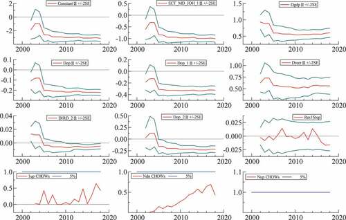
The first eight graphs in the figure show that all estimated coefficients are stable over time, including SoA representing the stability of the long-run relationship; further, none of the recursively estimated coefficients (red lines) demonstrate significant instability for most of the sample. None of the error bands of the two standard deviations (green lines) of the recursively estimated coefficients contain a zero line for most of the sample (the statistical significance of the coefficient on the change in the interest rate differential increases and the coefficient becomes more stable from 2010). Additionally, the error bands of the coefficients become narrower toward the end of the sample. The ninth graph illustrates that the recursively estimated residuals are stable over the analysis period, as they do not cross the error band at any point of the sample and move around the zero line. Finally, the last three graphs illustrate the results of the one-step, breakpoint, and forecast Chow tests, respectively. All show that the null hypotheses of no breakpoint cannot be rejected in any year of the sample period, including 2016–2018, when domestic energy price and fiscal reforms were implemented, and oil prices declined tremendously. Therefore, we conclude that there is no structural break in the relationship that M2 establishes with its determinants during 1989–2018.

4.6.2. Predictive ability of the final ECM specification

Here, we test the predictive ability of the final ECM specification selected by Autometrics. For 2019, the values of M2, GDP, PGDP, IRSA, OP and REER are taken from SAMA (2020), and the value of IRUK is calculated as the 5-year average. To challenge the predictive ability of the final ECM at a great extent, we re-estimate it until 2015 and leave 2016–2019, a period of large-scale reforms and oil price declines, for forecasting. Table 6 shows that the re-estimated final ECM specification has well-behaved residuals and almost the same coefficients as the full sample estimation in Table 5.

Table 6. Re-estimated final ECM specification

Regressor	Coefficient	Standard error
$\mathrm{\Delta m}2r_{\mathit{t}-1}$	−0.271***	0.058
$\mathrm{\Delta m}2r_{\mathit{t}-2}$	−0.321***	0.064
C	−3.082***	0.223
$\mathit{EC}{T}_{\mathit{t}-1}$	−1.001***	0.072
$\mathrm{\Delta gd}{p}_t$	0.564***	0.069
$\mathrm{\Delta o}{p}_t$	−0.221***	0.014
$\mathrm{\Delta o}{p}_{\mathit{t}-1}$	−0.336***	0.034
$\mathrm{\Delta ree}{r}_t$	0.576***	0.082
$\mathrm{\Delta IR}{D}_{\mathit{t}-2}$	−0.006**	0.002
$\mathrm{\Delta o}{p}_{\mathit{t}-2}$	−0.233***	0.035
$\mathit{DP}{2004}_t$	0.072***	0.014
$\mathit{DP}{2009}_t$	0.055***	0.015
Post-estimation test results
$F_{\mathit{SC}}=1.236\left[0.325\right]$; $F_{\mathit{ARCH}}=0.041\left[0.841\right]$; $F_{\mathit{HETR}}=1.416\left[0.374\right]$; $\mathit{\chi }{2}_N=1.940\left[0.379\right]$; $F_{\mathit{FF}}=0.095\left[0.910\right]$

Notes: $\mathrm{\Delta }$ m2r is the dependent variable; $F_{\mathit{SC}},F_{\mathit{ARCH}},F_{\mathit{HETR}},F_{\mathit{FF}}$ denote the F statistics to test the null hypotheses of no serial correlation, no autoregressive conditioned heteroskedasticity, no heteroskedasticity in the residuals and no functional form misspecification and no cointegration in the Wald test, respectively; $\mathit{\chi }{2}_N$ indicates the Chi-squared statistic to test the null hypothesis of the normal distribution of residuals. The values between brackets are the probabilities of the associated tests. Estimation period: 1990–2015.

Additionally, Figure 3 illustrates that the re-estimated final ECM specification approximates the actual growth rates of the real M2 aggregate well, especially if turning points are considered. Moreover, the scaled residuals do not show any significant outliers during 1990–2015.

Figure 3. Actual and modeled $\mathrm{\Delta m}2\mathit{r}$ and scaled residuals.

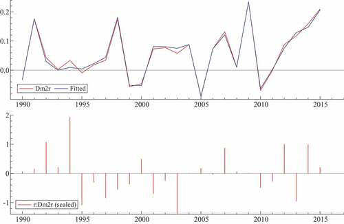
Therefore, Table 6 and Figure 3 show that the explanatory variables in the final ECM specification selected by Autometrics have reasonable power in explaining the $\mathrm{\Delta }$m2r dynamics.

During 2016–2019, Saudi Arabia experienced two waves of energy price reforms, in 2016 and 2018, and implemented an expat levy and value added tax in 2017 and 2018, respectively. The volatility of the Saudi economy due to these reforms, among other factors, makes the forecasting exercise quite difficult. For instance, the GDP growth rate slowed from 4.1% in 2015 to 1.7% in 2016, and even turned negative (–0.7%) in 2017 before rising (2.4%) in 2018 and then weakening once more (0.3%) in 2019. The growth rates of the real price of Arab light crude oil recovered from – 17.5% in 2016 to 26.4% and 27.8% in 2017 and 2018, respectively, but dropped to – 6.0% in 2019. The growth rates of the GDP deflator also varied significantly: – 3.05%, 7.4%, 11.9% and 0.3% for 2016–2019, respectively.

We selected the dynamic forecast option, which makes it more difficult for the model to predict out of sample values for the dependent variable compared to the static forecast option. For the forecast standard errors, we selected the error variance with parameter uncertainty. Note that other options, such as a one-step ahead forecast or forecast standard errors without parameter uncertainty, yield very similar outcomes. Figure 4 illustrates the actual (red line) and predicted (blue line) values of $\mathrm{\Delta }$m2r with an error band, that is, the predicted values plus/minus two times the forecast standard errors (green line) over 2016–2019.

Figure 4. Actual and forecasted $\mathrm{\Delta }\mathit{m}2\mathit{r}$.

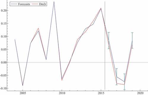
All actual $\mathrm{\Delta }$m2r values are inside the forecast error band. Additionally, the calculated t-ratios for the differences between the forecasted and actual values of $\mathrm{\Delta }$m2r for these years are – 1.1, – 1.6, – 0.7 and – 0.9, indicating that the differences are not statistically significant. These suggest that the final ECM specification has a reasonable predictive ability, although the period is quite volatile.

5. Discussion

The unit root test results showed that m2, gdp, pgdp, IRSA, IRD, op and reer are non-stationary, but their first differences are stationary; that is, they are all I(1) processes. From the results of the Johansen and ADL bounds tests, we conclude that there is one cointegrated relationship among the variables, meaning the variables move together over time as they share a common trend. Therefore, the relationship between the (log) levels of the variables is not spurious, and the estimated coefficients are valid for discussion and policy recommendations.

To extract more information from the data and obtain robust conclusions, we empirically analyzed the (1B3) and (1B6) equations alongside (1). Here, we discuss the empirical results of equation (1)(1) $\mathit{m}{r}_t^s=a_0+a_1{y}_t+a_2\mathit{e}{r}_t+a_3\mathit{o}{p}_t+a_4\mathit{IR}{D}_t+a_5{t}_t+e_t$(1) , because it is our preferred MD specification. Overall, our results are consistent with the combination of MD theory, the literature survey and country-specific features. We found that ceteris paribus, a 1% increase in GDP leads to a 0.7% increase in the demand for the real M2 money balance in the long run (see Table 4). The data do not satisfactorily support either the income unity hypothesis or half income unity (Baumol-Tobin) hypothesis. This shows that money velocity is unstable. As one of the anonymous referees mentioned, and as concluded by several studies, it is difficult to have a stable money velocity, as money is largely endogenous in modern economics and is affected by many factors, including FI (Friedman, 2004; Nelson, 2007; Thornton, 1983). Ahumada and Garegnani (2002), among others, note that when the income/transaction elasticity of money is smaller than unity, it empirically supports the negative effect of inflation tax on income distribution and indicates the level of the shadow economy. However, this is mostly the case when the cash in circulation is considered a measure of money, whereas we consider broad money in this study. As theoretically expected, income has a statistically significant positive impact on M2. This implies that transaction motives are at play in the Saudi economy. Specifically, economic agents demand more money to spend on goods and services when they have larger incomes. Our finding on the sign and significance of elasticity is in line with earlier Saudi MD studies reported in Table 1B, especially those using M2 and GDP as measures of money and income. Regarding the magnitude of elasticity, our estimate is close to that of Mahmood and Asif (2016), Basher and Fachin (2014), Masih and Algahtani (2008) and Nagadi (1985), who estimated the GDP elasticity of M2 to range from 0.61 to 1.2. Mahmood and Asif (2016) also found it to vary between 0.5 and 1 for Qatar, Oman, Kuwait and Bahrain. However, our numerical value is significantly different from the estimates of Bahmani (2008) and Al Rasasi and Banafea (2018), 2.11 and 1.94, respectively. This difference can be associated with the different analysis periods. For example, Al Rasasi and Banafea (2018) employed quarterly data from 2000 to 2016, while Bahmani’s (2008) sample ended in 2004. Additionally, they did not test the income-unity or half-unity hypotheses, which might have affected their findings.

Panel A of Table 4 shows that a 1%-point increase in the interest rate differential decreases demand for real M2 money by 1% in the long run. This is theoretically consistent with the opportunity cost of money. Definition-wise, an increase in IRD means that the interest rates in the U.K. are higher than those in Saudi Arabia (see Table 2). This will encourage the individuals in Saudi Arabia to consider investing in the U.K. because of the higher return. As a result, their demand for M2 will decline. The negative coefficient of the interest rate spread may also imply that the amount of money flowing from Saudi Arabia to other countries is greater than the money returning to Saudi Arabia from the assets in the U.K. in the long run. This is reasonable because, first, the rate of return on deposits and other assets in advanced economies, such as the U.K., is usually not as high as in emerging economies. Second, it is possible that agents investing abroad prefer to keep most of their returns in abroad. Although we did not find any Saudi MD study that uses interest rate differentials, our findings corroborate the MD studies on other countries (see, e.g., Bjørnland, 2005 for Venezuela; Rother, 1998; 1999 for the West African Monetary Union).

We found that a 1% increase in the international Arabian crude oil price causes a 0.1% expansion in the demand for real M2 in the long run. The statistically significant positive impact of oil price on the Saudi economy, including the MD, corresponds to its role in the country’s economic activity. Many studies have found that oil prices and revenues positively influence the development of the Saudi economy. An oil price rise increases demand for local currency in two stages. Oil constitutes around 85% of government revenue, and government spending is the main driver of economic activity (Al Moneef & Hasanov, 2020; Hasanov, AlKathiri, Alshahrani, & Alyamani, 2020a). First, according to Saudi law, all domestic transactions must be realized in SAR. Hence, the government must convert oil revenues from USD to SAR before spending them for budget purposes, which increases demand for SAR. Second, an expansion in government spending will boost economic activity, thus requiring more liquidity. The demand for money will also increase. To our best knowledge, of the Saudi studies, only Alsamara, Mrabet, Dombrecht, and Barkat (2017) include oil price in the MD analysis; they find its long-run impact to be around 0.05, which is not very different from ours (0.08).

According to Table 4, the demand for real M2 increases by 0.5% if the REER of Saudi Arabia increases by 1%. Recall that an increase in REER means that SAR appreciates against the currency basket of its main trading partners. In other words, the appreciation of SAR leads to increased local currency demand. This finding is consistent with MD theory, which articulates that ERs act as the opportunity costs of local currency and create a currency substitution effect. This means that, when SAR appreciates, individuals will prefer holding SAR over foreign currencies, as the former has higher purchasing power. They will also convert their foreign currency deposits into SAR. These consequently increase demand for SAR. The opposite is true when SAR REER depreciates. If the SAR depreciates, individuals will also demand more SARs to convert into foreign currencies to realize international transactions. It seems that this effect is dominated by the other effects previously mentioned, as the net effect of REER appreciation on M2 is found to be positive. Our finding is in line with earlier MD studies on Saudi Arabia, including Al-Bassam (1990), Hamdi, Said, and Sbia (2015), Mahmood and Asif (2016) and Al Rasasi and Banafea (2018), who use real ERs in their M2 analyses. The elasticities estimated by the latter two papers are close to ours.

Finally, we find a positive effect of FI, proxied by the time trend, on the M2 demand. Numerically, a 1% increase in the elements of FI (which change over time but are not explicitly included in the analysis) causes a 3% increase in M2. It is noteworthy that the magnitude of the effect does not change considerably regardless of whether real or nominal money balances are considered or whether a basic or an open economy augmented MD specification is estimated. Our explanation is that FI can be categorized into institutional, process and product innovations. Institutional innovations refer to the creation of new types of financial firms such as electronic trading platforms or specialist credit card firms, while product innovation involves creating new products such as foreign currency mortgages or securitization. Thus, we believe that process innovations dominate in Saudi Arabia (e.g., online banking, telephone banking and other novel financial and banking services). In support of our explanation, Albatel (2003) and AlYousef (2014), the only available studies that investigate the MD effects of FI in Saudi Arabia, do not discuss any institutional or product innovations when explaining the impact of the latter on the former. Instead, Albatel (2003) discusses government bonds and treasury bills, which he admits are not a part of FI. Online banking, telephone banking, online payments and other modern banking services prevail in Saudi Arabia. They encourage economic agents to increase their transactions significantly, which results in a higher demand for the M2 balance. Additionally, the time trend can be thought of as a collection of other factors that change over time, such as institutional and technological developments, and increased efficiencies in the these may in turn increase demand for money (see, e.g., Ericsson, 1998 for a more in-depth discussion).

Regarding the short-run relationship, the final ECM specification from Autometrics reported in Table 5 shows that $\mathit{EC}{T}_{\mathit{t}-1}$, contemporaneous values of Δgdp and Δreer, contemporaneous and 1- and 2-year lagged values of Δop, and 2-year lagged value of ΔIRD have statistically significant impacts on $\mathrm{\Delta }$m2r. The statistically significant SoA on $\mathit{EC}{T}_{\mathit{t}-1}$ is theoretically coherent, as it has a negative sign. This shows that the short-run deviations of real M2 from its long-run money market equilibrium relationship due to shocks or fluctuations are not permanent and will revert to the money market equilibrium. In other words, the long-run real MD relationship between M2R and its determinants (GDP, OP, REER and IRD) is stable, and any shocks to this relationship will be temporary. The size of the SoA indicates that 100% of the deviation in the previous year will be corrected in the present year. Earlier MD studies on Saudi Arabia, such as Nagadi (1985), Al-Bassam (1990), Masih and Algahtani (2008) and AlYousef (2014) – and Mahmood and Asif (2016) on Bahrain – also find a fast adjustment.

The final ECM shows that an increase in the contemporaneous growth rates of income and REER appreciation leads to an increase in the growth rates of the real M2. Increases in the contemporaneous and lagged growth rates of the real oil price, and in the lagged change of the interest rate spread, are negatively associated with the growth rates of real M2. Sign-wise, the short-run impacts of income, REER and interest rate spread are the same as those in the long run. However, this is not the case for the growth rates of real oil price. Graph A in Figure 5 illustrates a clear inverse association between the growth rates of the real oil price and real M2, with a correlation coefficient of – 0.81.

Figure 5. Time profiles of the growth rates of OP, M2R and GDPW.

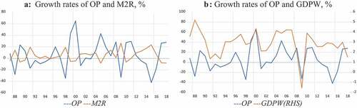
This negative relationship can be explained as follows. When oil price growth increases, the government obtains more oil revenues and transfers a major portion of these to the budget for public spending, while the rest is deposited as monetary reserve. From Graph B in Figure 5, and as discussed in the literature, a high aggregate demand and activity in the global economy drive up the oil price (e.g., He, Wang, & Lai, 2010; Kilian, 2009). The expansion of global economic activity (GDPW) and high oil prices should encourage not only the Saudi government but also Saudi households and firms to invest abroad to obtain higher returns.⁷ This will also happen because the investment opportunities in Saudi Arabia were not as attractive as in advanced and several developing economies because, like in many developing countries, the Saudi financial market was not so well developed historically. This will reduce the demand for SAR and increase demand for foreign currencies.

In the short run, the negative relationship between the growth rates of real oil price and real money balance does not necessarily imply that the levels of these variables are negatively related. This is because it is possible for the growth rate of a variable to decline, while its level continues to increase. In fact, as discussed previously, the levels of these variables are positively related; that is, an increase in the level of real oil prices causes an increase in the level of real money balance in the long run. High oil prices increase the government’s oil revenues and, when the government spends domestically, this leads to a high demand for SAR. At the same time, high oil prices are associated with increased global economic activity (more money moving from Saudi Arabia overseas), thereby increasing demand for foreign currencies and decreasing demand for SAR. In the short run, the second effect overweighs the first, resulting in a negative relationship. However, in the long run, the first effect will dominate the second, and the relationship will become positive. Indeed, the outflow of money from Saudi Arabia takes a short time to materialize, whereas additional demand for SAR caused by high oil prices takes more time. This is because oil revenues must first be approved by authorities and then go to the government budget before being injected into the economy.

Another explanation for the negative relationship between the growth rates of the variables is the prevailing temporary effect of the short-run relationship between variables, as Bjørnland (2005) discusses. Like our case, she estimates a statistically significant long-run negative relationship between the real M2 balance and bilateral ERs, which becomes statistically significant and positive in the short run. The same is also true for the relationship between the real M2 balance and the spread between domestic and foreign interest rates – she finds statistically significant positive and negative impacts of the latter on the former in the long and short run, respectively. She explains that some relationships are temporary in the short-run, and it takes time for them to switch as traditionally expected.

We found that the long-run elasticity of income is larger than the short-run elasticity (i.e., the coefficient on the contemporaneous growth rates). The opposite is true for the REER. This implies that the influences of income and REER in shaping the MD in Saudi Arabia increase and decrease, respectively, over time. Moreover, it is not necessary that the short-run elasticity always be smaller than the long-run elasticity (see, e.g. Kennedy, 2008; Hendry, 2020; Pesaran et al., 2001).

Finally, we conducted a stability analysis, employing various stability tests for robustness, to examine whether there is a break in the MD relationship we estimated. We also tested the predictive ability of the estimated MD specification. The results of the tests and forecasting indicated that the relationship between real M2 and its drivers (e.g., income, interest rate spread, oil price and REER) is stable over the considered period. This means that no policy or other economic shock, including the recent domestic reforms and the sharp drops in oil price, has created any structural breaks in the relationship that broad money establishes with its determinants. Our finding of a stable MD relationship is supported by many earlier Saudi studies.

6. Concluding remarks and policy insights

In line with its aim and objectives, this study shows that the MD relationship in fixed ER regimes differs from that in floating ER regimes by surveying studies in both regimes. As a case study, a relevant MD function for Saudi Arabia – a country with a fixed ER – is then specified and estimated, and its stability and predictive ability tested. The study empirically shows that an open economy model augmented with country-specific factors is a better framework to represent the MD function in a fixed ER economy. The numerical findings may be useful for Saudi MP authorities to better understand the MD relationship both in the short and long run. This understanding may help in implementing relevant MP to maintain macroeconomic stability, especially the stability of the fixed ER, which has become important for diversifying the non-oil economy. Policymakers should consider that other factors, besides those theoretically predicted, influence MD. This is important, first, because adequate money supply should be provided as oversupply or supply shortage could create pressure on the pegged ER and thus harm macroeconomic stability. Second, the stability of MD must be checked so that appropriate policy decisions can be made.

For Saudi Arabia, oil prices as a country-specific factor play an important role in the formation of MD in addition to the other determinants in an open-economy model.⁸ The main channel for injecting oil revenues into the economy is government spending, and fiscal policy occupies a dominant position in the Saudi economy, as in many other oil-exporting economies. Government spending is also an effective measure to stimulate economic growth in fixed ER economies. Therefore, monetary authorities should adjust the money supply in response to changes in oil prices and government spending. Authorities should also consider how to best manage foreign exchange reserves resulting from oil price changes. This is important because foreign exchange reserves are the main MP instrument for intervening in the foreign exchange market to maintain the stability of the currency peg in fixed ER regimes.

Finally, the monetary authorities should note that the relationship between real M2 and real income, interest rate differential, real oil price, FI and REER is stable over time, even during the recent period of economic reforms and oil price decline. This stability is key to monitoring MD fluctuations, which allows monetary authorities to maintain the required level of liquidity. As Alsamara et al. (2017) state, the existence of a stable MD relationship is a necessary condition for Saudi policymakers if they wish to switch to a flexible ER regime and target monetary aggregates or inflation. However, such a policy move seems impractical in Saudi Arabia, as the fixed ER regime has greatly served the country’s economic development in terms of macroeconomic stability and economic confidence (particularly in maintaining investor confidence and reducing inflationary pressures), which are key factors for successful economic transformation and non-oil sector diversification and expansion (see, e.g., Alkhareif, William, & Qualls, 2017; Banafe & Macleod, 2017; IMF, 2019; Ramady, 2010).

Acknowledgments

The authors thank SAMA workshop participants for their feedback. We would like also to thank Frederick Joutz as well as the editor of this journal and two anonymous referees for their comments and suggestions. The views expressed in this study are those of the authors and do not necessarily represent the views of their affiliated institutions. The authors are responsible for all errors and omissions.

Disclosure statement

No potential conflict of interest was reported by the author(s).

Supplementary material

Supplemental data for this article can be accessed here

Correction Statement

This article has been republished with minor changes. These changes do not impact the academic content of the article.

Notes

¹ A detailed discussion of the assumptions, features, advantages and disadvantages of a fixed ER regime compared to a floating ER regime, and MP under this regime type, is beyond the scope of this study but is well documented in the literature (see, e.g., Argy, McKibbin, & Siegloff, 1989; Krugman & Obstfeld, 2009; Walsh, 2017).

² The SAR/USD rate was fixed at 4.5 from 1960–1971, fluctuated around 3.5 from 1972–1986 and has been fixed at 3.75 since 1987, according to World Bank data.

³ Financial innovation refers to any developments in financial sector products that lead to lower costs or reduced risk for financial institutions or better services from the financial system.

⁴ In the bibliography of Albatel (2003), we came across Al-Bazai (1998), but since only the abstract was available, we did not include it in our survey.

⁵ For example, the Johansen test may indicate no cointegration. This may be due to the small sample size, as this method is based on a vector autoregressive (VAR) model, which requires many degrees of freedom. In such cases, we use ADLBT to ensure robustness.

⁶ Results of the cointegration and post-estimation tests and specified VAR models are available from the authors upon request.

⁷ Government overseas investments are handled by the Public Investment Fund (PIF), the eighth-largest sovereign wealth fund globally, with total assets of USD 390 billion (https://www.swfinstitute.org/fund-rankings/sovereign-wealth-fund). Note that two of PIF’s largest funding sources (capital injections from the government and government assets transferred to PIF) are based mainly on oil revenues.

⁸ To keep the section brief, following the recommendation by an anonymous referee, the policy implications of the findings for real income, prices, interest rate differentials, FI and REER are not discussed, as these implications are quite standard.

References

- Ahumada, H., & Garegnani, M. L. (2002, May 9–10). Understanding money demand of Argentina: 1935– 2000 [paper presentation]. VII Jornadas de Economía Monetaria e Internacional [VII Conference on Monetary and International Economics], La Plata, Argentina.
- Ahumada, H., & Garegnani, M. L. (2010, March 18 – 19). Selecting the money deflator by an encompassing approach: The case of Argentina [paper presentation]. 8th OxMetrics user conference, Washington, D.C., USA.
- Ahumada, H. A., & Garegnani, M. L. (2012). Forecasting a monetary aggregate under instability: Argentina after 2001. International Journal of Forecasting, 28(2), 412–427.
- Al Moneef, H. E., & Hasanov, F. (2020). Fiscal multipliers for Saudi Arabia revisited (KAPSARC Discussion Paper, No. ks–2020-dp21). King Abdullah Petroleum Studies and Research Center.
- Al Rasasi, M., & Banafea, W. A. (2018). Estimating money demand function in Saudi Arabia: Evidence from cash in advance model (Working Paper, No. WP/18/4). Saudi Arabian Monetary Agency.
- Al-Bassam, K. A. (1990). Money demand and supply in Saudi Arabia: An empirical analysis [ PhD Thesis, University of Leicester]. https://leicester.figshare.com/articles/thesis/Money_Demand_and_Supply_in_Saudi_Arabia_An_Empirical_Analysis_/10082438
- Al-Bazai, H. A. (1998). The demand for money in Saudi Arabia: Assessing the role of financial innovation. Journal of Economics and Administrative Sciences – UAE, 14, 79–106.
- Al-Jasser, M., & Banafe, A. (1999). Monetary policy instruments and procedures in Saudi Arabia. BIS Policy Papers, 5, 203–217.
- Al-Qudah, A. M. (2019). The determinants of money demand in Jordan: ARDL approach. Journal of Management Research, 11(1), 61–78.
- Albatel, A. (2003). Demand for money in a small open economy. Riyadh: King Saud University. https://cba.ksu.edu.sa/sites/cba.ksu.edu.sa/files/imce_images/eco_17.pdf
- Ali, I. (2017). Estimating the demand for money in Libya: An application of the Lagrange multiplier structural break unit root test and the ARDL cointegration approach. Applied Econometrics, 46, 126–138.
- Alkhareif, R., William, A. B., & Qualls, J. (2017). Has the dollar peg served the Saudi economy well? International Finance and Banking, 4(1), 145.
- Alsamara, M. (2011). An empirical analysis of the money demand function in Syria. Paris: Economic Centre of Sorbonne, University of Paris-1 Panthéon-Sorbonne.
- Alsamara, M., Mrabet, Z., Dombrecht, M., & Barkat, K. (2017). Asymmetric responses of money demand to oil price shocks in Saudi Arabia: A non-linear ARDL approach. Applied Economics, 49(37), 3758–3769.
- AlYousef, N. (2014). Stability of money demand in Saudi Arabia. Journal of Administrative Sciences, 26(2), 97–110.
- Andersen, A. B. (2004). Money demand in Denmark 1980–2002 (Working Paper, No. 18). Danmarks National Bank.
- Argy, V., McKibbin, W. J., & Siegloff, E. (1989). Exchange-rate regimes for a small economy in a multi-country world International finance section. United States: Department of Economics, Princeton University.
- Arrau, P., De Gregorio, J., Reinhart, C. M., & Wickham, P. (1995). The demand for money in developing countries: Assessing the role of financial innovation. Journal of Development Economics, 46(2), 317–340.
- Badinger, H. (2004). Austria’s demand for international reserves and monetary disequilibrium: The case of a small open economy with a fixed ER regime. Economica, 71(281), 39–55.
- Bahmani, S. (2008). Stability of the demand for money in the Middle East. Emerging Markets Finance & Trade, 44(1), 62–83.
- Bahmani-Oskooee, M., & Bahmani, S. (2015). Nonlinear ARDL approach and the demand for money in Iran. Economics Bulletin, 35(1), 381–391.
- Bahmani-Oskooee, M., & Ng, R. C. W. (2002). Long-run demand for money in Hong Kong: An application of the ARDL model. International Journal of Business and Economics, 1(2), 147.
- Bai, J., & Perron, P. (1998). Estimating and testing linear models with multiple structural changes. Econometrica, 66(1), 47–78.
- Banafe, A., & Macleod, R. (2017). Currency regime and monetary policy. In The Saudi Arabian Monetary Agency, 1952-2016 (pp. 225–244). Cham: Palgrave Macmillan.
- Basher, S. A., & Fachin, S. (2014). Investigating long-run demand for broad money in the Gulf Arab Countries. Middle East Development Journal, 6(2), 199–214.
- Bhatta, S. R. (2011). Stability of demand for money function in Nepal: A cointegration and error correction modeling approach (MPRA Paper, No. 41404). Munich Personal RePEc Archive.
- Bjørnland, H. C. (2005). A stable demand for money despite financial crisis: The case of Venezuela. Applied Economics, 37(4), 375–385.
- Blomqvist, A. G. (1970). A note on the appropriate use of monetary and fiscal policy under fixed ERs. The Swedish Journal of Economics, 72(4), 269–277.
- Breitung, J. (2001). “The local power of some unit root tests for panel data”. In Baltagi, B.H., Fomby, T.B., and Carter Hill, R. (Ed.), Nonstationary Panels, Panel Cointegration, and Dynamic Panels (Advances in Econometrics, Vol. 15, pp. 161–177), Emerald Group Publishing Limited, Bingley. doi:10.1016/S0731-9053(00)15006-6.
- Brouwer, G. D., & Ericsson, N. R. (1995). Modeling inflation in Australia (Research Discussion Paper, No. 9510/International Finance Discussion Paper, No. 530). Reserve Bank of Australia.
- Brouwer, G. D., & Ericsson, N. R. (1998). Modeling inflation in Australia. Journal of Business and Economic Statistics, 16(4), 433–449.
- Brown, R. L., Durbin, J., & Evans, J. M. (1975). Techniques for testing the constancy of regression relationships over time. Journal of the Royal Statistical Society B, 37, 149–163.
- Budha, B. B. (2011). An empirical analysis of money demand function in Nepal. NRB Economic Review, Nepal Rastra Bank, Research Department, 23(1), 54–70.
- Campos, J., Ericsson, N. R., & Hendry, D. F. (2005). General-to-specific modeling: An overview and selected bibliography (International Finance Discussion Papers, No. 838). Board of Governors of the Federal Reserve System.
- Carrera, C. (2016). Long-run money demand in Latin American countries: A nonstationary panel data approach. Monetaria, 4(1), 121–152.
- Chow, G. C. (1960). Tests of equality between sets of coefficients in two linear regressions. Econometrica, 28(3), 591–605.
- Coppin, A. (1991). The role of openness in the demand for money: Evidence from Barbados. North American Review of Economics & Finance, 2(2), 167–172.
- Curtis, D., & Irvine, I. (2021). Principles of microeconomics, 2021A version (Lyryx). Calgary, Alberta, Canada: Lyryx Learning.
- Darrat, A. F., & Al-Mutawa, A. (1996). Modelling money demand in the United Arab Emirates. The Quarterly Review of Economics and Finance, 36(1), 65–87.
- Dickey, D. A., & Fuller, W. A. (1979). Distribution of the estimators for autoregressive time series with a unit root. Journal of the American Statistical Association, 74(366), 427–431.
- Doornik, J. A. (2009). Autometrics. In J. L. Castle, and N. Shephard (Eds.), The methodology and practice of econometrics: A festschrift in honour of David F. Hendry (pp. 88–121). Oxford, United Kingdom: Oxford University Press.
- Doornik, J. A., & Hendry, D. F. (2018). Empirical econometric modelling using PcGive (Vol. I). United Kingdom: Timberlake Consultants Press.
- Edet, B. N., Udo, S. U., & Etim, O. U. (2017). Modelling the demand for money function in Nigeria: Is there stability? Bulletin of Business and Economics, 6(1), 45–57.
- Engle, R. F., & Granger, C. W. (1987). Co-integration and error correction: representation, estimation, and testing. Econometrica: journal of the Econometric Society, 251–276.
- Ericsson, N. R. (1998). Empirical modeling of money demand. Empirical Economics, 23(3), 295–315.
- Ericsson N R and MacKinnon J G. (2002). Distributions of error correction tests for cointegration. Econometrics Journal, 5(2), 285–318. 10.1111/1368-423X.00085
- Farazmand, H., Ansari, M. S., & Moradi, M. (2016). What determines money demand: Evidence from MENA. Economic Review, 45(2), 151–169.
- Friedman, M. (2004). Reflections on a monetary history. The Cato Journal, 23(3), 349–352.
- General Authority for Statistics, Kingdom of Saudi Arabia (GaStat). (2020). Gross domestic product. Retrieved 2020, from https://www.stats.gov.sa/en/823
- Gonand, F., Hasanov, F. J., & Hunt, L. C. (2019). Estimating the impact of energy price reform on Saudi Arabian intergenerational welfare using the MEGIR-SA model. The Energy Journal, 40(3). doi:10.5547/01956574.40.3.fgon
- Hamdi, H., Said, A., & Sbia, R. (2015). Empirical evidence on the long-run money demand function in the Gulf Cooperation Council countries. International Journal of Economics and Financial Issues, 5(2), 603–612.
- Hamori, S. (2008). Empirical Analysis of the Money Demand Function in Sub-Saharan Africa. Economics Bulletin, AccessEcon, 15(4), 1–15.
- Hansen B E. (1992). Testing for parameter instability in linear models. Journal of Policy Modeling, 14(4), 517–533. doi:10.1016/0161-8938(92)90019-9.
- Harb, N. (2004). Money demand function: A heterogeneous panel application. Applied Economics Letters, 11(9), 551–555.
- Hasanov, F. J., AlKathiri, N., Alshahrani, S., & Alyamani, R. (2020a). The impact of fiscal policy on non-oil GDP in Saudi Arabia (KAPSARC Discussion Paper, No. ks–2020-dp14). King Abdullah Petroleum Studies and Research Center.
- Hasanov, F. J., Joutz, F., Mikayilov, J., & Javid, M. (2020b). KGEMM—A macroeconometric model for Saudi Arabia (KAPSARC Discussion Paper, No. ks–2020-dp04). King Abdullah Petroleum Studies and Research Center.
- He, Y., Wang, S., & Lai, K. K. (2010). Global economic activity and crude oil prices: A cointegration analysis. Energy Economics, 32(4), 868–876.
- Hendry, D.F. (2020). First In, First Out: Econometric Modelling of UK Annual CO2 Emissions (pp. 1860-2017). University of Oxford
- Hendry, D. F. (2018). Deciding between alternative approaches in macroeconomics. International Journal of Forecasting, 34(1), 119–135.
- Hendry, D. F., & Johansen, S. (2015). Model discovery and Trygve Haavelmo’s legacy. Econometric Theory, 31, 93–114.
- Hendry, D. F., Johansen, S., & Santos, C. (2008). Automatic selection of indicators in a fully saturated regression (with erratum). Computational Statistics, 23(2), 317–335, 337–339.
- Hoover, K. D., Johansen, S., & Juselius, K. (2008). Allowing the data to speak freely: The macroeconometrics of the cointegrated vector autoregression. American Economic Review, 98(2), 251–255.
- Hossain, A. A. (2019). How justified is abandoning money in the conduct of monetary policy in Australia on the grounds of instability in the money‐demand function? Economic Notes: Review of Banking, Finance and Monetary Economics, 48(2), e12131.
- Im K So, Pesaran M and Shin Y. (2003). Testing for unit roots in heterogeneous panels. Journal of Econometrics, 115(1), 53–74. doi:10.1016/S0304-4076(03)00092-7.
- International Monetary Fund (IMF). (2019). Saudi Arabia: 2019 Article IV consultation—Press release and staff report (Country Report, No. 19/290). IMF.
- Jackman, M. (2010). Money demand and economic uncertainty in Barbados (MPRA Paper, No. 34561). Munich Personal RePEc Archive.
- Jayaraman, T. K., & Ward, B. D. (2000). Demand for money, financial reforms and monetary policy in Fiji: An econometric analysis (Discussion Paper, No. 53). Commerce Division, Lincoln University.
- Johansen, S. (1988). Statistical analysis of cointegration vectors. Journal of Economic Dynamics & Control, 12(2–3), 231–254.
- Johansen, S., & Juselius, K. (1990). Maximum likelihood estimated and inference on cointegration with application to the demand for money. Oxford Bulletin of Economics and Statistics, 52(2), 169–210.
- Kao, C. (1999). Spurious regression and residual-based tests for cointegration in panel data. Journal of Econometrics, 90(1), 1–44.
- Katafono, R. (2001). A re-examination of the demand for money in Fiji. Economics Department, Reserve Bank of Fiji.
- Kennedy, P. (2008). A guide to econometrics. John Wiley & Sons.
- Kilian, L. (2009). Not all oil price shocks are alike: Disentangling demand and supply shocks in the crude oil market. American Economic Review, 99(3), 1053–1069.
- Krugman, P. R., & Obstfeld, M. (2009). International economics: Theory and policy. London, United Kingdom: Pearson Education.
- Lee, C., Chang, C., & Chen, P. (2008). Money demand function versus monetary integration: Revisiting panel cointegration among GCC countries. Mathematics and Computers in Simulation, 79(1), 85–93.
- Lee, J., & Strazicich, M. C. (2003). Minimum Lagrange multiplier unit root test with two structural breaks. Review of Economics and Statistics, 85(4), 1082–1089.
- Levin A, Lin C and James Chu C. (2002). Unit root tests in panel data: asymptotic and finite-sample properties. Journal of Econometrics, 108(1), 1–24. doi:10.1016/S0304-4076(01)00098-7.
- Lieberman, C. (1977). The transactions demand for money and technological change. The Review of Economics and Statistics, 59(3), 307–317.
- MacKinnon, J. G. (1996). Numerical distribution functions for unit root and cointegration tests. Journal of Applied Econometrics, 11(6), 601–618.
- Maddala. G. S and Wu S. (1999). A Comparative Study of Unit Root Tests with Panel Data and a New Simple Test. Oxford Bulletin of Economics and Statistics, 61(S1), 631–652. doi:10.1111/1468-0084.0610s1631.
- Mahmood, H., & Asif, M. (2016). An empirical investigation of stability of money demand for GCC countries. International Journal of Economics and Business Research, 11(3), 274–286.
- Mala, B. L. (2014). Money demand estimation for Fiji (Working Paper, No. EGWP 2014-01). Reserve Bank of Fiji.
- Mankiw, N. G. (2003). Macroeconomics (5th ed.). New York, United States: Worth Publishers.
- Marquez, J. (1987). Money demand in open economies: A currency substitution model for Venezuela. Journal of International Money and Finance, 6(2), 167–178.
- Masih, M., & Algahtani, I. (2008). Estimation of long-run demand for money: An application of long-run structural modeling to Saudi Arabia. International Economics, 61(1), 81–99.
- Mundell, R. A. (1960). The monetary dynamics of international adjustment under fixed and flexible ERs. The Quarterly Journal of Economics, 74(2), 227–257.
- Mundell, R. A. (1962). The appropriate use of monetary and fiscal policy for internal and external stability. Staff Papers, 9(1), 70–79.
- Nachega, J. (2001). A Cointegration Analysis of Broad Money Demand in Cameroon. IMF Working Papers, 01(26). doi:10.5089/9781451844382.001.
- Nagadi, A. H. (1985). Demand for money in Saudi Arabia: An empirical study [ Unpublished Ph.D. dissertation]. Claremont Graduate School, U.S.A.
- Narayan, P. K., & Narayan, S. (2008). Estimating the demand for money in an unstable open economy: the case of the Fiji Islands. Economic Issues, 13(1), 71–91.
- Narayan, P. K. (2005). The saving and investment nexus for China: Evidence from cointegration tests. Applied Economics, 37(17), 1979–1990.
- Narayan, P. Kumar, Narayan, S, and Mishra, V. (2009). Estimating money demand functions for South Asian countries. Empir Econ, 36(3), 685–696. doi:10.1007/s00181-008-0219-9.
- Nelson, E. (2007). Milton Friedman and US monetary history. Federal Reserve Bank of St. Louis Review, 89(3), 153–182.
- Nielsen, B. (2008). On the explosive nature of hyper-inflation data. Economics: The Open-Access, Open-Assessment E-Journal, 2(1), 2008–2021.
- Onafowora, O. A., & Owoye, O. (2015). Structural adjustment and the stability of the Nigerian money demand function. International Business & Economics Research Journal, 3(8), 55–64.
- Oxford Economics (OEGEM). (2017, July). Oxford Economics Global Economic Model Database. London, United Kingdom. release.
- Pedroni, P. (2004). Panel cointegration: asymptotic and finite sample properties of pooled time series tests with an application to the PPP hypothesis. Econ. Theory, 20(03). doi:10.1017/S0266466604203073.
- Pesaran, M. H., & Shin, Y. (1998). An autoregressive distributed-lag modelling approach to cointegration analysis. Econometric Society Monographs, 31, 371–413.
- Pesaran, M. H., Shin, Y., & Smith, R. P. (2001). Bounds testing approaches to the analysis of level relationships. Journal of Applied Econometrics, 16(3), 289–326.
- Phillips, P. C. B., & Perron, P. (1988). Testing for unit toots in time series regression. Biometrika, 75(2), 335–346.
- Ramady, M. A. (2010). Saudi Arabian monetary agency (SAMA) and monetary policy. In The Saudi Arabian economy (pp. 75–109). Boston, USA: Springer.
- Reinsel, G. C., & Ahn, S. K. (1992). Vector autoregressive models with unit roots and reduced rank structure: Estimation, likelihood ratio test, and forecasting. Journal of Time Series Analysis, 13(4), 353–375.
- Rother, P. C. (1998). Money demand and reginal monetary policy in the West African Economic and Monetary Union (IMF Working Paper, No. WP/98/57). International Monetary Fund.
- Rother, P. C. (1999). Money demand in the West African Economic and Monetary Union—The problem of aggregation. Journal of African Economies, 8(3), 422–477.
- Saed, A. A., & Al-Shawaqfeh, W. (2017). The stability of money demand function in Jordan: Evidence from the autoregressive distributed lag model. International Journal of Economics and Financial Issues, Econjournals, 7(5), 331–337.
- Saudi Central Bank (SAMA). 2020. Yearly Statistics. https://www.sama.gov.sa/en-US/EconomicReports/Pages/YearlyStatistics.aspx
- Sheefeni, J. P. S. (2013). Demand for money in Nambia: An ARDL bounds testing approach. Asian Journal of Business and Management, 1(3), 65–71.
- Swoboda, A. K. (1973). Monetary policy under fixed ERs: Effectiveness, the speed of adjustment and proper use. Economica, 40(158), 136–154.
- Taylor, J. B. (2019). Inflation targeting in high inflation emerging economies: Lessons about rules and instruments. Journal of Applied Economics, 22(1), 102–115.
- Thornton, D. L. (1983). Why does velocity matter. Missouri, United States: Federal Reserve Bank of St Louis.
- Walsh, C. E. (2017). Monetary theory and policy. Cambridge, Massachusetts, United States: MIT press.
- Westerlund, J. (2006). Testing for Panel Cointegration with Multiple Structural Breaks*. Oxford Bull Econ & Stats, 68(1), 101–132. doi:10.1111/j.1468-0084.2006.00154.x.
- The World Bank. (2020). The world development indicators. Washington, D.C., United States: Author.