On the sparsity of synthetic control method

ABSTRACT

Synthetic Control Method (SCM) is a popular approach for causal inference in panel data, where the optimal weights for control units are often sparse. But the sparsity of SCM has received little attention in the literature except Abadie (2021), which explores the sparsity from the perspective of predictor space. In this paper, we make three contributions. First, we show that if there is a unique solution, then the number of positive weights is upper-bounded by the number of covariates. Second, we offer a simple alternative explanation about the sparsity of SCM from the perspective of parameter space. Third, we conduct a meta-analysis of empirical studies using SCM in the literature, which shows that the sparsity of SCM decreases with the relative number of covariates. A practical implication is that if the number of positive weights exceeds the number of covariates, there are multiple solutions and possibly unstable weights.

KEYWORDS:

• Synthetic control method
• sparsity
• meta-analysis

1. Introduction

Synthetic control method (SCM) is a popular approach for causal inference in panel data with a single treated unit (Abadie & Gardeazabal, 2003; Abadie et al., 2010), which has found many applications in fields such as economics, politics and health. For a treated unit, SCM constructs its counterfactual outcomes via a convex combination of control units, i.e., a linear combination with nonnegative weights summed to one. In practice, the optimal weights are usually sparse such that the share of zero weights are high. Obviously, sparsity of weights makes the interpretation of SCM easy. As pointed out by Abadie (2021, p. 407), “sparsity plays an important role for the interpretation and evaluation of the estimated counterfactual”.

However, there has been little formal discussion about the sparsity of SCM until Abadie (2021), which explains the origin of sparsity from the perspective of predictor space. In this paper, we make three contributions in understanding the sparsity of SCM. First, we show that if there is a unique solution, then the number of positive weights cannot exceed the number of covariates, which yields a lower bound for the sparsity defined as the share of zero weights. Second, we offer a simple alternative explanation about the sparsity. Viewed from the perspective of parameter space, the sparsity of SCM arises simply because the feasible parameter space is a probability simplex with sharp vertices, similar to the sparsity of Lasso in origin. Third, we conduct a meta-analysis of empirical studies using SCM in the literature, and show that consistent with our theoretical finding, the sparsity of SCM decreases with the relative number of covariates as a fraction of the number of control units.

The rest of the paper is organized as follows. Section 2 reviews the methodology of SCM. Section 3 explores the sparsity of SCM from the perspective of predictor space, and derives a lower bound for sparsity when there is a unique solution. Section 4 proposes an alternative explanation of sparsity from the perspective of parameter space. Section 5 conducts a meta-analysis of empirical studies using SCM in the literature, which yields results consistent with our theoretical finding. Section 6 provides a discussion and guidance to empirical practice, and section 7 concludes.

2. Synthetic control method

Suppose there are $\mathit{N}+1$ cross-sectional units indexed by $\mathit{i}=1,\cdots ,\mathit{N}+1$ and observed over periods $\mathit{t}=1,\cdots ,T_0$ (pre-intervention) and$\mathit{t}=T_0+1,\cdots ,\mathit{T}$ (post-intervention). The first unit $(\mathit{i}=1)$ is the treated unit, while all other units $(\mathit{i}=2,\cdots ,\mathit{N}+1)$ are control units, which forms the donor pool. Let $y_{it}^1$ and $y_{it}^0$ be the outcome of unit $\mathit{i}$ in period $\mathit{t}$ with and without intervention respectively, and${\mathrm{\Delta }}_{\mathit{it}}=y_{it}^1-y_{it}^0$ is the corresponding treatment effect. SCM seeks to approximate the unknown $y_{1t}^0(\mathit{t}=T_0+1,\cdots ,\mathit{T})$ by a weighted average of control units, and the treatment effects are estimated by

(1) ${\hat{\mathrm{\Delta }}}_{1\mathit{t}}=y_{1\mathit{t}}-{\hat{y}}_{1\mathit{t}}^0=y_{1\mathit{t}}-\sum _{\mathit{i}=2}^{\mathit{N}+1}{w}_i{y}_{\mathit{it}}(\mathit{t}=T_0+1,\cdots ,\mathit{T}),$(1)

where $\mathbf{w}=(w_2\cdots w_{\mathit{N}+1}){ }^{\mathrm{\prime }}$ is a $\mathit{N}\times 1$ vector of weights (a potential synthetic control) such that $0\le w_i\le 1$ for $\mathit{i}=2,\cdots ,\mathit{N}+1$ and ${\sum }_{i=2}^{N+1}{w}_i=1$.

Let ${\mathbf{x}}_1$ be the $\mathit{K}\times 1$ vector containing the pretreatment covariates (also known as predictors) of the treated unit,¹ and ${\mathbf{X}}_0$ be the $\mathit{K}\times \mathit{N}$ matrix containing the pretreatment covariates of the $\mathit{N}$ control units. SCM selects the optimal ${\mathbf{w}}^{\ast }$ such that the pretreatment characteristics of the synthetic control are most similar to that of the treated unit. Specifically, the optimal synthetic control ${\mathbf{w}}^{\ast }$ is obtained by solving the following minimization problem:

(2) ${\mathbf{w}}^{\ast }=\underset{\mathbf{w}}{argmin}{\left({\mathbf{x}}_1-{\mathbf{X}}_0\mathbf{w}\right)}^{\mathrm{\prime }}\mathbf{V}\left({\mathbf{x}}_1-{\mathbf{X}}_0\mathbf{w}\right),$(2)

where $\mathbf{V}$ is a $\mathit{K}\times \mathit{K}$ diagonal matrix with nonnegative elements on its diagonal, which measures the relative importance of each covariate in predicting the outcome. The optimal $\mathbf{V}$ can be determined by minimizing the mean squared prediction error (MSPE) of the outcome variable during the pretreatment period. See Abadie et al. (2010) for details of implementation.

3. The sparsity of SCM viewed from the predictor space

Consider the minimization problem in Equation (2)(2) ${\mathbf{w}}^{\ast }=\underset{\mathbf{w}}{argmin}{\left({\mathbf{x}}_1-{\mathbf{X}}_0\mathbf{w}\right)}^{\mathrm{\prime }}\mathbf{V}\left({\mathbf{x}}_1-{\mathbf{X}}_0\mathbf{w}\right),$(2) along with constraints on the weights:

(3) $\begin{array}{rl}& \underset{\mathbf{w}}{min}{\left({\mathbf{x}}_1-{\mathbf{X}}_0\mathbf{w}\right)}^{\mathrm{\prime }}\mathbf{V}\left({\mathbf{x}}_1-{\mathbf{X}}_0\mathbf{w}\right),\\ & \mathit{\hspace{0.17em}}\mathit{s}.\mathit{t}.\mathbf{w}\ge 0,\mathit{\iota }{ }^{\mathrm{\prime }}\mathbf{w}=1\end{array}$(3)

where $\mathit{\iota }=(1\cdots 1){ }^{\mathrm{\prime }}$ is a $\mathit{N}$ dimensional vector consisting of all ones. Abadie (2021) proposes an explanation about the sparsity of SCM from the perspective of predictor space. Define $\mathit{H}({\mathbf{X}}_0)$ as the convex hull of the columns of ${\mathbf{X}}_0$, i.e., the smallest convex set containing the columns of ${\mathbf{X}}_0$; or equivalently, the intersection of all convex sets containing the columns of ${\mathbf{X}}_0$. Specifically, $\mathit{H}({\mathbf{X}}_0)$ can be defined as

(4) $\mathit{H}({\mathbf{X}}_0)\equiv \left\{{\mathbf{X}}_0\mathbf{w}:\mathit{\hspace{0.17em}}\mathbf{w}\ge 0,\mathit{\iota }{ }^{\mathrm{\prime }}\mathbf{w}=1\right\}.$(4)

If ${\mathbf{x}}_1$ is in the convex hull, i.e., ${\mathbf{x}}_1\in \mathit{H}({\mathbf{X}}_0)$, then the objective function achieves a minimum of zero. In this case, we can find optimal weights ${\mathbf{w}}^{\ast }$ that perfectly reproduces the pretreatment characteristics of the treat unit, i.e., ${\mathbf{x}}_1-{\mathbf{X}}_0\mathbf{w}=\mathbf{0}$. We call the optimal weights ${\mathbf{w}}^{\ast }$ an “exact solution”.

For illustration, consider a simple case with $\mathit{K}=2$ (two covariates) and $\mathit{N}=5$ (five control units); see Figure 1. In Figure 1, ${\mathbf{x}}_1\in int\left(\mathit{H}({\mathbf{X}}_0)\right)$ (located in the interior of the convex hull) represents the covariates of the treated unit, while ${\mathbf{x}}_2,\cdots ,{\mathbf{x}}_6$ represent the covariates for units 2 through 6, and ${\mathbf{X}}_0=({\mathbf{x}}_2\cdots {\mathbf{x}}_6)$. In this case, it is easy to see that exact solutions ${\mathbf{w}}^{\ast }$ are not unique, since there are different convex combinations of ${\mathbf{x}}_2,\cdots ,{\mathbf{x}}_6$ that can perfectly reproduce ${\mathbf{x}}_1$. Therefore, the number of positive weights is only limited by the number of control units in general when there are exact solutions and ${\mathbf{x}}_1\in int\left(\mathit{H}({\mathbf{X}}_0)\right)$.

Figure 1. Multiple exact solutions.

Now consider the situation in Figure 2, where ${\mathbf{x}}_1$ is located on the boundary of the convex hull, i.e., ${\mathbf{x}}_1\in \mathrm{\partial }\left(\mathit{H}({\mathbf{X}}_0)\right)$. Clearly, there is a unique exact solution with positive weights for ${\mathbf{x}}_5$ and ${\mathbf{x}}_6$ respectively. When there is a unique exact solution and $\mathit{K}=2$ (as presented in Figure 2), there can be at most 2 positive weights, since two vertices in a two-dimensional space form an edge. Similarly, when there is a unique exact solution and $\mathit{K}=3$, there can be at most 3 positive weights, since three vertices in a three-dimensional space form a face. By the same reasoning, when there is a unique exact solution, the number of positive weights cannot exceed the number of covariates. We state this formally in Proposition 1 below with a proof.

Figure 2. A unique exact solution.

However, in empirical practice, ${\mathbf{x}}_1$ usually falls outside of the convex hull, i.e., ${\mathbf{x}}_1\notin \mathit{H}({\mathbf{X}}_0)$, which results in an “approximate solution”. In this case, the optimal weights ${\mathbf{w}}^{\ast }$ provides a prediction ${\mathbf{X}}_0{\mathbf{w}}^{\ast }$, which is a linear projection of ${\mathbf{x}}_1$ to $\mathit{H}({\mathbf{X}}_0)$. Thus, the sparsity of SCM arises because projection to a convex hull typically do not rely on all vertices, where each vertex represents a control unit, i.e., a column in ${\mathbf{X}}_0$; see Figure A1 in Abadie (2021), which is reproduced in Appendix 1 for convenience. Those control units with vertices making no contribution to the linear projection thus receive zero weights.

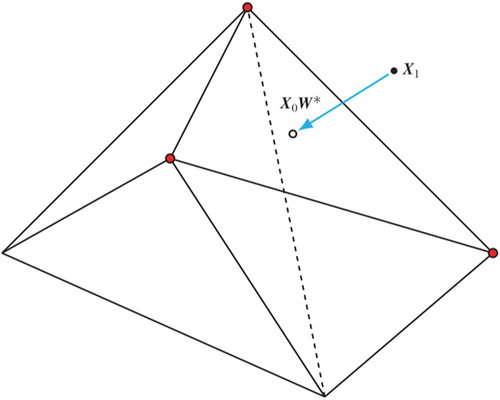
Consider again the case with $\mathit{K}=2$ (two covariates) and $\mathit{N}=5$ (five control units), but now there is a unique approximate solution on an edge (see Figure 3). In Figure 3, ${\mathbf{x}}_1$ falls outside the convex hull of ${\mathbf{X}}_0$. The linear projection to $\mathit{H}({\mathbf{X}}_0)$ results in two positive weights for ${\mathbf{x}}_2$ and ${\mathbf{x}}_6$ respectively, whereas ${\mathbf{x}}_3,{\mathbf{x}}_4,{\mathbf{x}}_5$ all receive zero weights.

Figure 3. A unique approximate solution on an edge.

In Figure 3, the number of positive weights and the number of covariates happen to be equal. Of course, the number of positive weights could be smaller than the number of covariates. For example, if the projection of ${\mathbf{x}}_1$ to $\mathit{H}({\mathbf{X}}_0)$ lands on a vertex, instead of any line segment connecting two vertices, then the number of positive weights drops to just one; see Figure 4.

Figure 4. A unique approximate solution on a vertex.

A further question is whether the number of positive weights can surpass the number of covariates. Geometrically, this appears to be impossible from Figure 3. In this case, the projection of ${\mathbf{x}}_1$ to $\mathit{H}({\mathbf{X}}_0)$ lies on the line segment connecting ${\mathbf{x}}_2$ and ${\mathbf{x}}_6$. Note that in any plane, a straight line passing through two different points cuts the plane into two half-planes. In our case, the straight line passing through ${\mathbf{x}}_2$ and ${\mathbf{x}}_6$ cuts the plane into two half-planes, such that the other vertices (i.e., ${\mathbf{x}}_3,{\mathbf{x}}_4,{\mathbf{x}}_5$) are in the open half-plane further away from ${\mathbf{x}}_1$ by definition (thus receiving zero weights), since the unique approximate solution lies on the line segment connecting ${\mathbf{x}}_2$ and ${\mathbf{x}}_6$ (thus receiving positive weights). Therefore, the number of positive weights cannot be more than 2 in this case.

The same reasoning applies to higher dimensions in general. For any fixed $\mathit{K}$, consider the $\mathit{K}$dimensional predictor space. When there is a unique approximate solution with $\mathit{K}$ positive weights, then the hyperplane passing through the corresponding $\mathit{K}$ vertices cuts the predictor space into two half-spaces, such that the other vertices are in the open half-space further away from ${\mathbf{x}}_1$ by definition (thus receiving zero weights), since the unique approximate solution lies on the face connecting the $\mathit{K}$ vertices with positive weights. Therefore, the number of positive weights cannot be larger than $\mathit{K}$ in this case. We state this result formally below, and give a rigorous proof by contradiction.

Proposition 1.

Consider a synthetic control problem with $\mathit{K}$ covariates and $\mathit{N}$ control units, and $\mathit{N}>\mathit{K}$. If there is a unique solution (either exact or approximate), then the number of positive weights are less than or equal to $\mathit{K}$.

Proof.

We prove by contradiction. Denote $N_p$ as the number of positive weights. Suppose there is a unique solution (either exact or approximate), but $N_p>\mathit{K}$. Without loss of generality, assume that the first $N_p$ control units $\left\{{\mathbf{x}}_2,\cdots ,{\mathbf{x}}_{N_p+1}\right\}$ receive positive weights, whereas all the rest control units $\left\{{\mathbf{x}}_{N_p+2},\cdots ,{\mathbf{x}}_N\right\}$ get zero weights.

Denote ${\mathbf{X}}_0^{(1)}\equiv ({\mathbf{x}}_2\cdots {\mathbf{x}}_{N_p+1})$, and note that ${\mathbf{X}}_0^{(1)}$ is a $\mathit{K}\times N_p$ matrix with row rank less than or equal to $\mathit{K}$. Thus the column rank of ${\mathbf{X}}_0^{(1)}$ is also less than or equal to $\mathit{K}$, which in turn is strictly less than $N_p$ by assumption:

$\mathit{colrank}\left({\mathbf{X}}_0^{(1)}\right)=\mathit{rowrank}\left({\mathbf{X}}_0^{(1)}\right)\le \mathit{K}<N_p.$

Therefore, the $\mathit{K}\times N_p$ matrix ${\mathbf{X}}_0^{(1)}$ does not have a full column rank, so its columns $\left\{{\mathbf{x}}_2,\cdots ,{\mathbf{x}}_{N_p+1}\right\}$ are strictly multicollinear. Hence, the solution to synthetic control problem is not unique, which leads to a contradiction.

An immediate implication of Proposition 1 is that if the number of positive weights exceeds the number of covariates, then the solutions to the synthetic control problem under consideration are not unique. Therefore, applied researchers should be concerned if the number of positive weights is larger than the number of covariates, which is symptomatic of the existence of multiple solutions. As a way out, one may change the model specification by adding more covariates or dropping multicollinear control units (more on this below), until the number of positive weights are less than or equal to the number of covariates.

Proposition 1 gives an upper bound on the number of positive weights, which naturally yields a lower bound on the number of zero weights. Since this paper is primarily concerned with the sparsity of SCM, denote $N_z$ as the number of zero weights, such that $\mathit{N}=N_p+N_z$. Moreover, define the sparsity of SCM as the share of zero weights, i.e., $N_z/\mathit{N}$. From Proposition 1, we immediately have the following proposition.

Proposition 2.

Consider a synthetic control problem with $\mathit{K}$ covariates and $\mathit{N}$ control units, and $\mathit{N}>\mathit{K}$. If there is a unique solution, then the sparsity of SCM satisfies the following inequality:

(5) $1-\frac{K}{N}\le \mathit{sparsity}\le 1-\frac{1}{N}.$(5)

Proof.

First, according to Proposition 1, $N_p\le \mathit{K}$, which implies $N_z\ge \mathit{N}-\mathit{K}$. Divide both sides of this inequality by $\mathit{N}$, and rearranging, we have $\mathit{sparsity}=\frac{N_z}{\mathit{N}}\ge 1-\frac{K}{N}$.

Second, since there needs to be at least one positive weight, the largest possible value of $N_z$ is $(\mathit{N}-1)$, thus $\mathit{sparsity}=\frac{N_z}{\mathit{N}}\le 1-\frac{1}{N}$

From the above discussion, it is clear that when there is a unique solution, the lower bound for sparsity given by $\left(1-\frac{K}{N}\right)$ could be tight in some cases, as long as the optimal solution resides on a regular face of the convex hull (which is usually a polyhedron or polytope), instead of on a lower-dimensional edge or vertex.

Also note that an important condition for Proposition 1 is the uniqueness of solution. On the contrary, if the solutions are not unique, then the number of positive weights can be larger than the number of covariates, and it is only limited by the number of control units; see Figure 5. In Figure 5, ${\mathbf{x}}_2,{\mathbf{x}}_3,{\mathbf{x}}_5,{\mathbf{x}}_6$ line up in a straight line. Clearly, multiple solutions are now available. In particular, it is possible to assign positive weights to control units ${\mathbf{x}}_2,{\mathbf{x}}_3,{\mathbf{x}}_5,{\mathbf{x}}_6$ as an optimal solution. In practice, this is the optimal solution that is often found by quadratic programming algorithms in used (say, the algorithm used by the Stata command synth), which results in many small positive weights that are far from being sparse. In fact, even if ${\mathbf{x}}_2,{\mathbf{x}}_3,{\mathbf{x}}_5,{\mathbf{x}}_6$ does not perfectly line up in a straight line, as long as the iterative algorithm thinks they are, the same result would follow. In the presence of (near) multicollinearity, a simple fix is to drop control units that are most responsible for (near) multicollinearity.² For example, dropping ${\mathbf{x}}_2$ and ${\mathbf{x}}_6$ in Figure 5 would solve the problem, and obtain a unique solution.

Figure 5. Approximate solutions that are not unique.

To illustrate the above results, we revisit the case study on the effect of California’s tobacco control program (Abadie et al., 2010). We use the Stata command synth for synthetic control estimation,³ while incrementally increasing the number of covariates from one to seven, which is the same as specified in Abadie et al. (2010). The results are reported in Table 1.

Table 1. A case study of California’s tobacco control program.

$\mathit{N}$	$\mathit{K}$	$N_p$	$N_z$	Covariates
38	1	38	0	retprice
38	2	2	36	retprice, lnincome
38	3	3	35	retprice, lnincome, age15to24
38	4	4	34	retprice, lnincome, age15to24, beer
38	5	5	33	retprice, lnincome, age15to24, beer, cigsale(1975)
38	6	4	34	retprice, lnincome, age15to24, beer, cigsale(1975), cigsale(1980)
38	7	4	34	retprice, lnincome, age15to24, beer, cigsale(1975), cigsale(1980), cigsale(1988)

For variable definitions, refer to Abadie et al. (2010).

In Table 1, when there is only one covariate ($\mathit{K}=1$), the algorithm returns all small positive weights (ranging from 0.016 to 0.11) without any zero weight. Apparently, when $\mathit{K}=1$, ${\mathbf{X}}_0$ is just a $1\times \mathit{N}$ matrix such that all columns of ${\mathbf{X}}_0$ are perfectly collinear, which line up in a straight line. Clearly, multiple solutions are available, and the algorithm just spews out a solution in a seemingly random way. On the other hand, when $2\le \mathit{K}\le 7$, the number of positive weights $N_p$ is always upper-bounded by $\mathit{K}$, where this upper bound is sometimes obtained. While this example is somewhat artificial,⁴ this is not a trivial case in practice. In fact, in the meta-analysis in Section 5, we find that among 658 empirical studies using SCM in the sample, 4.56% of them have weights that are all positive.⁵

Furthermore, since unique solution appears to be frequent in practice, while the lower bound $\left(1-\frac{K}{N}\right)$ in Proposition 2 may be tight in some cases, we propose the following hypothesis to be tested by the meta-analysis in Section 5.

Hypothesis 1.

Other things being equal, the sparsity of SCM decreases with the relative number of covariates as a fraction of the number of control units (i.e., $\mathit{K}/\mathit{N}$) in empirical studies.

4. The sparsity of SCM viewed from the parameter space

Before moving to the meta-analysis in Section 5, we propose a simple alternative explanation of the sparsity of SCM from the perspective of parameter space in this section. First, note that the feasible set of weights is actually a probability simplex defined as $\left\{\mathbf{w}:\mathbf{w}\ge 0,\mathit{\iota }{ }^{\mathrm{\prime }}\mathbf{w}=1\right\}$. Second, the objective function is a quadratic form with a nonnegative diagonal matrix as its matrix. Thus, the contour sets of the objective function are ellipses or ellipsoids in high dimensions. For example, when there are only two control units (i.e., $\mathit{N}=2$), the minimization problem can be geometrically represented in Figure 6.

Figure 6. Optimal synthetic control in the 2D parameter space.

In Figure 6, the contour sets are ellipses with axes parallel to the coordinate axes, since no cross-terms are involved in the quadratic form of the objective function. Due to the constraint$\left\{\mathbf{w}:\mathbf{w}\ge 0,\mathit{\iota }{ }^{\mathrm{\prime }}\mathbf{w}=1\right\}$, the feasible parameter space is the line segment connecting $(1,0)$ and $(0,1)$. ${\mathbf{w}}^{\ast \ast }$ is the unconstrained optimum, whereas ${\mathbf{w}}^{\ast }$ is the constrained optimum, which is a sparse solution with $w_2^{\ast }=0$ and $w_3^{\ast }=1$. Apparently, the sparsity of SCM arises simply because the feasible parameter set is a probability simplex with sharp vertices (in this case pointed ends). In a way, the origin of the sparsity of SCM is reminiscent of the sparsity of Lasso, where the feasible parameter space is of a diamond shape with sharp vertices. Of course, it is still possible for the optimal solution to lie in the middle of the line segment connecting $(1,0)$ and $(0,1)$, but the presence of sharp vertices makes it less likely. Similarly, when there are only three control units (i.e., $\mathit{N}=3$), the minimization problem can be geometrically represented in Figure 7.

Figure 7. Optimal synthetic control in the 3D parameter space.

In Figure 7, the contour sets are ellipsoids with axes parallel to the coordinate axes. The feasible parameter space is the face of a polyhedron connecting three vertices $(1,0,0)$, $(0,1,0)$, and$(0,0,1)$. The optimal synthetic control is a sparse solution with $w_2^{\ast }=w_4^{\ast }=0$ and $w_3^{\ast }=1$. Again, the sparsity of SCM arises because of the sharp vertices of the feasible parameter space. Apparently, similar situations hold in higher dimensions, although we cannot draw graphs when there are more than three control units.

5. A meta-analysis

In this section, we conduct a meta-analysis of empirical studies using SCM in the literature. We search JSTOR and ScienceDirect with the keyword “synthetic control”, and obtain a sample of 107 empirical papers using SCM published during 2003–2022 across disciplines such as economics, political science, health and environment.⁶ Note that some papers using SCM do not report the number of positive weights, and are thus not included in the sample. While these papers certainly do not exhaust all empirical studies using SCM to date, they are sufficient for our purpose. Among the 107 papers in the sample, 61 of them conducted multiple SCM studies, thus we end up with 658 observations. Among these 61 papers, 39 out of them conducted SCM studies for different treated units, while the rest 22 papers applied SCM to different outcome variables.⁷

As before, denote$\mathit{N}$, $\mathit{K}$, $N_p$ and $N_z$ as the number of control units, the number of covariates, the number of positive weights, and the number of zero weights respectively. The dependent variable sparsity is defined as the share of zero weights, i.e., sparsity = $N_z/\mathit{N}$. The summary statistics are reported in Table 2. As revealed by Table 2, the number of control units ($\mathit{N}$) ranges from as few as 4 to as many as 326. On the other hand, the number of covariates ($\mathit{K}$) has much less variation, ranging from 3 to 27. Our key explanatory variable $\left(\mathit{K}/\mathit{N}\right)$ has a mean of 0.522, but with a relatively large standard deviation of 0.369. The number of positive weights ranges from 1 to 54, whereas the number of zero weights ranges from as few as 0 to as many as 319.

Table 2. Summary statistics.

Variable	Observations	Mean	Std. Dev.	Min	Max
$\mathit{N}$	658	26.588	23.975	4	326
$\mathit{K}$	658	9.336	4.479	3	27
$\mathit{K}/\mathit{N}$	658	0.522	0.369	0.0215	3.25
$N_p$	658	5.784	6.491	1	54
$N_z$	658	20.792	23.959	0	319
sparsity ($N_z/\mathit{N}$)	658	0.698	0.257	0	0.991

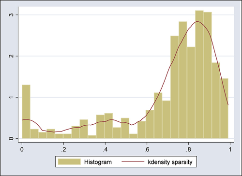
The dependent variable sparsity ($N_z/\mathit{N}$) has a mean of 0.698, implying that the share of zero weights is 69.8% on average. However, the range of sparsity is quite wide, spanning from 0 to 0.991. Moreover, Figure 8 presents a histogram and a kernel density plot of sparsity. Clearly, most empirical studies using SCM have sparse weights. However, there are also some studies characterized by “dense” weights, i.e., there are more positive weights than zero weights. In particular, there are 30 studies (4.56% of the sample) with zero sparsity, i.e., all weights are positive and there is no zero weight.

Figure 8. The distribution of sparsity.

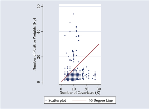
Next, we explore the relation between the number of positive weights ($N_p$) and the number of covariates ($\mathit{K}$). Figure 9 presents a scatterplot along with a 45 degree line. It is clear that most points are located below the 45 degree line satisfying $N_p\le \mathit{K}$, which is largely consistent with Proposition 1. In fact, among 658 SCM studies in the sample, 88.9% of them (585 studies) satisfy $N_p\le \mathit{K}$. For the rest 11.1% of them (73 studies) with $N_p>\mathit{K}$, there are multiple and potentially unstable weights according to Proposition 1.

Figure 9. The numbers of positive weights and covariates.

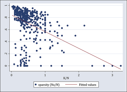
Before conducting regression analysis, Figure 10 provides a scatterplot and a linear fit between the dependent variable sparsity and the key explanatory variable $\left(\mathit{K}/\mathit{N}\right)$. Consistent with Hypothesis 1, they are negatively correlated. The coefficient of correlation is −0.397, which is significant at 1%.

Figure 10. The number of positive weights and the number of covariates.

To test Hypothesis 1 more rigorously, we consider the following regression specification:

(6) $\mathit{sparsit}{y}_{\mathit{ij}}={\beta }_0+{\beta }_1\left(K_{\mathit{ij}}/N_{\mathit{ij}}\right)+{\beta }_2{K}_{\mathit{ij}}+{\beta }_3{N}_{\mathit{ij}}+{\beta }_4\left(K_{\mathit{ij}}\times N_{\mathit{ij}}\right)+u_i+{\epsilon }_{\mathit{ij}},$(6)

where the subscripts “$\mathit{ij}$” refer to paper $\mathit{i}$’s jth SCM study, and $u_i$ represents paper fixed effects, which can be controlled by adding dummies for all but the first papers.⁸ The key explanatory variable $\left(K_{\mathit{ij}}/N_{\mathit{ij}}\right)$ is theoretically motivated by Hypothesis 1, while the rest regressors $K_{\mathit{ij}}$, $N_{\mathit{ij}}$ and $\left(K_{\mathit{ij}}\times N_{\mathit{ij}}\right)$ are typical terms used in reduced-form regressions. We take a general-to-specific approach to model selection, also known as the “sequential t-rule”.⁹ Specifically, we first estimate Equation (6)(6) $\mathit{sparsit}{y}_{\mathit{ij}}={\beta }_0+{\beta }_1\left(K_{\mathit{ij}}/N_{\mathit{ij}}\right)+{\beta }_2{K}_{\mathit{ij}}+{\beta }_3{N}_{\mathit{ij}}+{\beta }_4\left(K_{\mathit{ij}}\times N_{\mathit{ij}}\right)+u_i+{\epsilon }_{\mathit{ij}},$(6) by OLS, then drop the most insignificant variable each time, until all regressors are significant. The results are reported in Table 3.

Table 3. Results of OLS regressions.

Dependent Variable: sparsity	(1)	(2)	(3)	(4)
$\mathit{K}/\mathit{N}$	−0.243**	−0.238***	−0.258***	−0.224***
	(0.0937)	(0.0855)	(0.0902)	(0.0705)
$\mathit{K}$	0.0228	0.0199	0.0175
	(0.0183)	(0.0137)	(0.0134)
$\mathit{N}$	0.00285	0.00199
	(0.00332)	(0.00172)
$\mathit{K}\times \mathit{N}$	−0.000126
	(0.000320)
constant	0.762***	0.783***	0.859***	1.043***
	(0.161)	(0.134)	(0.106)	(0.0529)
paper fixed effects	Yes	Yes	Yes	Yes
N	658	658	658	658
R^2	0.571	0.571	0.570	0.567
Adjusted R^2	0.485	0.486	0.486	0.483

Standard errors clustered at the paper level are in parentheses.

*p < 0.1, **p < 0.05, ***p < 0.01.

As shown in Table 3, the coefficient of $\left(\mathit{K}/\mathit{N}\right)$ is negatively significant at 5% or 1%, and the magnitudes are very stable across different specifications. This lends support to Hypothesis 1, i.e., the sparsity of SCM decreases with the relative number of covariates as a fraction of the number of control units. On the other hand, all other regressors (except the constant term) are insignificant throughout.

However, since the dependent variable sparsity is bounded between 0 and 1, this is an example of limited dependent variable. Thus, a linear regression model may be misspecified, since it places no restriction on the dependent variable. For example, the predicted outcome could take values outside the interval $[0,1]$. Therefore, as a robustness check, we next consider fractional response models such as fractional probit and fractional logit (Papke & Wooldridge, 1996, 2008; Wooldridge, 2010), which are fit by quasi maximum likelihood estimation (QMLE).

The likelihood function for fractional probit (or fractional logit) is exactly the same as that of probit (or logit), except that the dependent variable may take on values in the interval $[0,1]$ instead of just 0 and 1. Moreover, as QMLE, fractional response models are consistently estimated as long as the conditional mean is correctly specified. The results of fractional probit and fractional logit regressions are reported in Tables 4 and 5 respectively, where the results are qualitatively similar to the results from OLS regressions reported in Table 3. Overall, the meta-analysis in this section confirms the negative relation between sparsity and the relative number of covariates, which supports Propositions 1 and 2, and the derived Hypothesis 1.

Table 4. Results of fractional probit regressions.

Dependent Variable: sparsity	(1)	(2)	(3)	(4)
$\mathit{K}/\mathit{N}$	−0.804**	−0.786***	−0.867***	−0.744***
	(0.320)	(0.283)	(0.306)	(0.223)
$\mathit{K}$	0.0700	0.0618	0.0572
	(0.0574)	(0.0423)	(0.0433)
$\mathit{N}$	0.00884	0.00645
	(0.0100)	(0.00494)
$\mathit{K}\times \mathit{N}$	−0.000377
	(0.00116)
constant	0.844*	0.895**	1.115***	1.708***
	(0.441)	(0.371)	(0.331)	(0.167)
paper fixed effects	Yes	Yes	Yes	Yes
N	658	658	658	658
Pseudo R^2	0.151	0.151	0.151	0.150

Standard errors clustered at the paper level are in parentheses.

*p < 0.1, **p < 0.05, ***p < 0.01.

Table 5. Results of fractional logit regressions.

Dependent Variable: sparsity	(1)	(2)	(3)	(4)
$\mathit{K}/\mathit{N}$	−1.276**	−1.257***	−1.405***	−1.217***
	(0.537)	(0.469)	(0.519)	(0.373)
$\mathit{K}$	0.108	0.100	0.0937
	(0.100)	(0.0736)	(0.0758)
$\mathit{N}$	0.0144	0.0120
	(0.0192)	(0.00967)
$\mathit{K}\times \mathit{N}$	−0.000400
	(0.00227)
constant	1.449*	1.495**	1.876***	2.859***
	(0.781)	(0.674)	(0.589)	(0.280)
paper fixed effects	Yes	Yes	Yes	Yes
N	658	658	658	658
Pseudo R^2	0.151	0.151	0.150	0.150

Standard errors clustered at the paper level are in parentheses.

*p < 0.1, **p < 0.05, ***p < 0.01.

6. Discussion

Proposition 1 implies that a necessary condition for a unique solution of the SCM problem is that the number of positive weights is less than or equal to the number of covariates. For applied researchers, this provides an easy check on the possibility of multiple solutions. Specifically, if the number of positive weights exceeds the number of covariates, then one should be concerned with the existence of multiple solutions, which may result in unstable and random weights.

A possible way to resolve the issue of multiple solutions is to change the model specification by adding more covariates, since too few covariates could result in unstable weights, which are symptomatic of multiple solutions. However, too many covariates are not necessarily helpful, since irrelevant covariates with little predictive power over the outcome variable would just get zero or very small weights in the quadratic form. Apparently, getting more relevant covariates is always helpful. Therefore, not only the number of covariates matters, but also their quality.

Another way to fix the problem of multiple solutions is to drop control units that are (nearly) multicollinear. As shown in Figure 5, (nearly) multicollinear control units could also result in multiple solutions. Specifically, one may conduct regressions among $\left\{{\mathbf{x}}_2,\cdots ,{\mathbf{x}}_{\mathit{N}+1}\right\}$ and drop the variable with the highest $R^2$, and so on. Hopefully, by adding more covariates or dropping multicollinear control units, the number of positive weights no longer exceeds the number of covariates, thus relieving the concern over multiple solutions.

7. Conclusion

The optimal weights for synthetic control estimation are often sparse in practice, but little explanation has been offered in the literature except Abadie (2021). To the best of our knowledge, this is the first paper devoted entirely to understanding the sparsity of SCM. Specifically, we make three contributions. First, from the perspective of predictor space, we show that if there is a unique solution, then the number of positive weights are upper-bounded by the number of covariates. Second, we offer a simple alternative explanation about the sparsity of SCM from the perspective of parameter space. Last but not least, we conduct a meta-analysis of empirical studies using SCM in the literature. Consistently with our theoretical finding, regression analysis shows that the sparsity of SCM decreases with the relative number of covariates as a fraction of the number of control units.

An important take-away from this paper is that if the number of positive weights exceeds the number of covariates (which happened for 11.1% SCM studies in our sample), then there are multiple solutions to the synthetic control problem, which may result in unstable and random weights. In this case, applied researchers are recommended to change the model specification by adding more covariates or dropping multicollinear control units until multiple solutions are no longer a concern.

Disclosure statement

No potential conflict of interest was reported by the author(s).

Additional information

Notes on contributors

Qiang Chen

Qiang Chen is a professor at the School of Economics, Shandong University.

Wenjun Li

Wenjun Li is a PhD student at the School of Economics, Shandong University.

Notes

¹ In this paper, we use the terms “covariate” and “predictor” interchangeably.

² One may regress among $\left\{{\mathbf{x}}_2,\cdots ,{\mathbf{x}}_{\mathit{N}+1}\right\}$ and drop the variable with the highest $R^2$, and so on.

³ For illustration purpose, we do not use the options “nested allopt” for more accurate numerical computation, otherwise the algorithm would fail when there is only one covariate (K = 1).

⁴ Note that Abadie et al. (2010) never estimates the one-covariate case.

⁵ Among these 30 studies with all positive weights, the number of covariates ranges from 3 to 14 with a mean of 9, and the number of control units ranges from 4 to 54 with a mean of 17.43.

⁶ See Appendix 2 for a complete list of these papers used in the meta-analysis.

⁷ Note that all 61 papers with multiple SCM studies used the same donor pools throughout, and 49 of them used the same covariates as well, but 12 of them used different covariates due to missing values.

⁸ The paper fixed effects term $u_i$ captures unobserved heterogeneity across papers, which is analogous to the individual fixed effects in the panel data setting. Since $u_i$ may be correlated with the regressors, its omission could result in inconsistent estimation. Moreover, since some paper dummies are significant in the regressions (unreported), the paper fixed effects specification is preferred over the pooled OLS.

⁹ The opposite specific-to-general approach starts from the smallest model possible (i.e., a model with only the constant term), and proceeds by adding the most significant regressor at each step. However, the specific-to-general approach may suffer from omitted variable bias when the model is too small.

Appendix 1.

Figure A1 in Abadie (2021)

Figure A1. Projecting $X_1$ on the convex hull of $X_0$.

Figure A1 in Abadie (2021) is reproduced here for convenience.

Appendix 2.

A list of papers used in the meta-analysis

Abadie, A., Gardeazabal, J., 2003. The Economic costs of conflict: A case study of the Basque Country. The Amer. Econ. Rev 93(1), 113-132.

Abadie, A., Diamond, A., Hainmueller, J., 2010. Synthetic control methods for comparative case studies: Estimating the effect of California’s tobacco control program. J. Amer. Statist. Assoc. 105(490),493–505.

Abadie, A., Diamond, A., Hainmueller, J., 2010. Comparative politics and the synthetic control method. Am. J. Polit. Sci. 59(2), 495–510.

Ando, M., 2015. Dreams of urbanization: Quantitative case studies on the local impacts of nuclear power facilities using the synthetic control method. J. Urb. Econ. 85,68-85.

Adhikari, B., Alm, J., 2016. Evaluating the economic effects of flat tax reforms using synthetic control methods. South. Econ. J. 83(2), 437-463.

Almer, C., Winkler, R., 2017. Analyzing the effectiveness of international environmental policies: The case of the Kyoto Protocol. J. Envi. Econ. Mana. 82,125–151.

Aytug, H., 2017. Does the reserve options mechanism really decrease exchange rate volatility? The synthetic control method approach. Inter. Rev. Econ. Fina. 51,405–416.

Azzolini, D., Guetto, R., 2017. The impact of citizenship on intermarriage: Quasi-experimental evidence from two European Union Eastern enlargements. Demographic Research 36, 1299-1336.

Andersson, J., J.,2019. Carbon taxes and CO₂ emissions. Amer. Econ. J. Econ. Pol. 11(4), 1-30.

Aboal, D., Crespi, G., and Perera, m.,2020. How effective are cluster development policies? Evidence from Uruguay. Wo. Deve. Pers. 18,1-17.

Absher, s., Grier, k., and Grier, r.,2020. The economic consequences of durable left-populist regimes in Latin America. J. Econ. Beha. Org. 177,787–817.

Alcocer, J., J.,2020. Exploring the effect of Colorado’s recreational marijuana policy on opioid overdose rates. Public Health 185,8-14.

Ayala, L., Javier Martín-Román, Navarro, C.,2022. Unemployment shocks and material deprivation in the European Union: A synthetic control approach. Economic Systems 10,1-18.

Bohn, S., Lofstrom, M., and Raphael, S.,2014. DID the 2007 legal Arizona Workers Act reduce the state’s unauthorized immigrant population? The Rev. Econ. Stat. 96(2), 258-269.

Bove, V., and Nisticò, R.,2014. Coups d’état and defense spending: a counterfactual analysis. Public Choice. 161(3/4), 321-344.

Bilgel, F., Galle, B., 2015. Financial incentives for kidney donation: A comparative case study using synthetic controls. J. Heal. Econ. 43,103-117.

Barone, G., David, F., and de Blasio, G., 2016. Boulevard of broken dreams. The end of EU funding (1997: Abruzzi, Italy). Regi. Scie. Urb. Econ. 60,31–38.

Bonander, C., Jakobsson, N., Podestà, F., and Svensson, M., 2016. Universities as engines for regional growth? Using the synthetic control method to analyze the effects of research universities. Regi. Scie. Urb. Econ. 60,198–207.

Brazil, N., 2016. Large-scale urban riots and residential segregation: A case study of the 1960s U.S. riots. Demography 53(2), 567-585.

Borbely, D., 2019. A case study on Germany’s aviation tax using the synthetic control approach. Trans. Res. Part A 126,377–395.

Baxter, A., J., Dundas, R., Popham, F., and Craig, P., 2021. How effective was England’s teenage pregnancy strategy? A comparative analysis of high-income countries. Soc. Scie. & Med. 270,1-9.

Becker, M., Pfeifer, G., and Schweikert, K., 2021. Price effects of the Austrian Fuel Price Fixing Act: A synthetic control study. Energy Economics 97,1-15.

Barber, A., West, J., 2022. Conditional cash lotteries increase COVID-19 vaccination rates. J. Heal. Econ. 81,1-14.

Bonander, C., Ekman.M, and Jakobsson, n., 2022. Vaccination nudges: A study of pre-booked COVID-19 vaccinations in Sweden. Soc. Scie. & Med. 309,1-11

Corral, L., R., Schling, M., 2017. The impact of shoreline stabilization on economic growth in small island developing states. J. Env. Econ. Mana. 86,210–228.

Castillo, V., Garone, L., F., Maffioli, A., and Salazar, L., 2017. The causal effects of regional industrial policies on employment: A synthetic control approach. Reg. Scie. Urb. Econ. 67,25–41.

Chamon, M., Garcia, M., and Souza, L., 2017. FX interventions in Brazil: A synthetic control approach. J. Inter. Econ. 108, 157–168.

Carbo, J., M., Graham, D., J.,2020. Quantifying the impacts of air transportation on economic productivity: a quasi-experimental causal analysis. Econ. Trans. 24,1-13.

Correa, J., Cisneros, E., Börner, J., Pfaff, A., Costa, M., and Rajão, r., 2020. Evaluating REDD at subnational level: Amazon fund impacts in Alta Floresta, Brazil. For. Pol. Econ. 116,1-9.

Chi Yuan-Ying, Wang Yuan-Yuan, and Xu Jin-Hua,2021. Estimating the impact of the license plate quota policy for ICEVs on new energy vehicle adoption by using synthetic control method. Energy Policy 149(2),1-13.

Chen Xing, Lin Boqiang,2021. Towards carbon neutrality by implementing carbon emissions trading scheme: Policy evaluation in China. Energy Policy 157,1-12.

Cappelli, F., Caravaggio, N., and C. Vaquero-Pi˜neiro, 2022. Buen Vivir and forest conservation in Bolivia: False promises or effective change? For. Pol. Econ. 137,1-15.

Chen Jiandong, Huang Shasha, Shen Zhiyang, Song Malin, and Zhu Zunhong, 2022. Impact of sulfur dioxide emissions trading pilot scheme on pollution emissions intensity: A study based on the synthetic control method. Energy Policy 161,1-11.

Di Xiang, Lawley, C., 2018. The impact of British Columbia’s carbon tax on residential natural gas consumption. Energy Economics 80,206–218.

Duarte, R., ´Alvaro García-Riazuelo, Luis Antonio S´aez, and Sarasa,C., 2022. Economic and territorial integration of renewables in rural areas: Lessons from a long-term perspective. Energy Economics 110,106005.

Eren, O., Ozbeklik, S., 2016. What do right-to-work laws do? Evidence from a synthetic control method analysis. J. Pol. Anal. Mana. 35(1), 173-194.

Eliason, P., Lutz, B., 2018. Can fiscal rules constrain the size of government? An analysis of the “crown jewel” of tax and expenditure limitations. J. Pub. Econ. 166,115–144.

Ezequiel Garcia-Lembergman, Rossi, M., A., and Stucchi R., 2018. The impact of export restrictions on production: A synthetic control approach. Economía 18(2),147-173.

Fremeth, R., A., Holburn, L., F., G., and Richter, K., B., 2016. Bridging qualitative and quantitative methods in organizational research: Applications of synthetic control methodology in the U.S. automobile industry. Organization Science 27(2), 462-482.

Freire, D., 2018. Evaluating the effect of homicide prevention strategies in São Paulo, Brazil. Lat. Amer. Res. Rev. 53(2), 231-249.

Grindal, T., Martin R. West, John B. Willett and Yoshikawa, H., 2015. The impact of home-based child care provider unionization on the cost, type, and availability of subsidized child care in Illinois. J. Pol. Anal. Mana. 34(4), 853-880.

Gharehgozli, O., 2017. An estimation of the economic cost of recent sanctions on Iran using the synthetic control method. Economics Letters 157,141–144.

Guo Jing, Zhang Zhengyu, 2019. Does renaming promote economic development? New evidence from a city-renaming reform experiment in China. China Economic Review 57,1-27.

Geloso, V., Pavlik, J., B., 2021. The Cuban revolution and infant mortality: A synthetic control approach. Exp. Econ. Hist. 80,1-9.

Gabriel Fuentes Cordoba,2022. The impact of the Panama Canal transfer on the Panamanian economy. Economics Letters 211,1-5.

Geloso, V., J., Grier, K., B., 2022. Love on the rocks: The causal effects of separatist governments in Quebec. Euro. J. Polit. Econ. 71,1-14.

Guan Huaping, Guo Binhua,2022. Digital economy and demand structure of skilled talents —analysis based on the perspective of vertical technological innovation. Tele. Infor. Rep. 7,1-8.

Hope, D., 2016. Estimating the effect of the EMU on current account balances: A synthetic control approach. Euro. J. Polit. Econ. 44,20–40.

Hu Hui, Zhu Yu-Qi, Li Si-Yue, and Li Zheng, 2021. Effects of green energy development on population growth and employment: Evidence from shale gas exploitation in Chongqing, China. Petroleum Science 18,1578-1588.

He Peiming, Zhang Jiaming, and Chen Litai, 2022. Time is money: Impact of China-Europe Railway Express on the export of laptop products from Chongqing to Europe. Transport Policy 125,312–322.

Joseph, J. Sabia, Richard, V. Burkhauser, and Ben., 2012. Are the effects of minimum wage increases always small? New evidence from a case study of New York state. ILR Review 65(2), 350-376.

Jones, B., A., 2018. Spillover health effects of energy efficiency investments: Quasi-experimental evidence from the Los Angeles LED streetlight program. J. Envi. Econ. Mana. 88,283–299.

Jakus, P., M., Akhundjanov, S., B., 2019. The Antiquities Act, national monuments, and the regional economy. J. Envi. Econ. Mana. 95,102–117.

Jarrett, U., Mohaddes, K., and Mohtadi, H., 2019. Oil price volatility, financial institutions and economic growth. Energy Policy 126,131–144.

Jones, B., A., Goodkind, A., L., 2019. Urban afforestation and infant health: Evidence from MillionTrees, NYC. J. Envi. Econ. Mana. 95,26-44.

Kennedy, R., 2014. Fading colours? A synthetic comparative case study of the impact of “Colour Revolutions”. Comparative Politics 46(3), 273-292.

Karlsson, M., Pichler, S., 2015. Demographic consequences of HIV. J. Pop. Econ. 28(4), 1097-1135.

Keller, m., 2022. Oil revenues vs domestic taxation: Deeper insights into the crowding-out effect. Resources Policy 76,1-26.

Lacono, R., 2016. No blessing, no curse? On the benefits of being a resource-rich southern region of Italy. Res Econ 70,346–359.

Luechinger, S., Roth, F., 2016. Effects of a mileage tax for trucks. J. Urb. Econ. 92, 1–15.

Lindo, J., M., Packham, A., 2017. How much can expanding access to long-acting reversible contraceptives reduce teen birth rates? Amer. Econ. J. Econ. Poli. 9(3), 348-376.

Lin Boqiang, Chen Xing, 2018. Is the implementation of the increasing block electricity prices policy really effective? - Evidence based on the analysis of synthetic control method. Energy 163,734-750.

Lee, K., Melstrom, R., T., 2018. Evidence of increased electricity influx following the regional greenhouse gas initiative. Energy Economics 76,127–135.

Li Xiaolong, Wu Zongfa, and Zhao Xingchen,2020. Economic effect and its disparity of high speed rail in China: A study of mechanism based on synthesis control method. Transport Policy 99,262–274.

Lee Wang-Sheng,2021. Comparative case studies of the effects of inflation targeting in emerging economies. Ox. Econ. Pap. 63(2), 375-397.

Lattanzio, G.,2022. Beyond religion and culture: The economic consequences of the institutionalization of sharia law. Emer. Mark. Rev. 52,1-19.

Leroutier, M., Carbon pricing and power sector decarbonization: Evidence from the UK. J. Envi. Econ. Mana. 111,1-22.

Lin Lee-Kai,2022. Effects of a global budget payment scheme on medical specialty workforces. Soc. Scie. & Med. 309,1-12.

Leng Xuan, Zhong Shihu, and Kang Yankun,2022. Citizen participation and urban air pollution abatement: Evidence from environmental whistle-blowing platform policy in Sichuan China. Scie. Tot. Envi. 816(4),1-13.

Munasib, A., Rickman, S., D., 2015. Regional economic impacts of the shale gas and tight oil boom: A synthetic control analysis. Reg. Scie. Urb. Econ. 50,1–17.

Man-Keun Kim, Kim, T., 2016. Estimating impact of regional greenhouse gas initiative on coal to gas switching using synthetic control methods. Energy Economics 59,328–335.

Maguire, K., Munasib, A., 2016. The disparate influence of state renewable portfolio standards on renewable electricity generation capacity. Land Economics 92(3), 468-490.

Mäkelä, E., 2017. The effect of mass influx on labor markets: Portuguese 1974 evidence revisited. Euro. Econ. Rev. 98,240–263.

Mohan, P., 2017. The economic impact of hurricanes on bananas: A case study of Dominica using synthetic control methods. Food Policy 68,21–30.

Marchesi, S., Masi, T.,2020. Sovereign rating after private and official restructuring, Economics Letters 192,1-7.

Monastiriotis, V., Zilic, I.,2020. The economic effects of political disintegration: Lessons from Serbia and Montenegro, Euro. J. Polit. Econ. 65,1-15.

Marinello, S., Leider, J., Pugach, O., and Powell, l., m.,2021. The impact of the Philadelphia beverage tax on employment: A synthetic control analysis. Econ. Hum. Biol. 40,1-9.

Matti, j., Yang Zhou,2021. Money is money: The economic impact of BerkShares, Ecological Economics 192,1-18.

Nowrasteh, A., Forrester, A., C.,2020. How U.S. travel restrictions on China affected the spread of COVID-19 in the United States. Cato Institute 8(58), 2-32.

Olper, A., Curzi, D., and Swinnen, J.,2017. Trade liberalization and child mortality: A synthetic control method. World Development 110,394–410.

Pinotti, P., 2015. The economic costs of organized crime: Evidence from southern Italy. The Econ. J. 125(586), F203-F232.

Puzzello, L., Pedro Gomis-Porqueras, 2018. Winners and losers from the €uro. Euro. Econ. Rev. 8,129–152.

Panagiotoglou, D., 2022. Using synthetic controls to estimate the population-level effects of Ontario’s recently implemented overdose prevention sites and consumption and treatment services. Inter. J. Dru. Poli. 110,1-11.

Pavlik, J., B., Jahan, I., and Young, A., T., 2022. Do longer constitutions corrupt? Euro. J. Polit. Econ. xxx,1-39.

Reimer, M., N., Guettabi, M., and Audrey-Loraine Tanaka, 2017. Short-run impacts of a severance tax change: Evidence from Alaska. Energy Policy 107,448–458.

Rickman, D., S., Hongbo Wang, and Winters, J., V., 2017. Is shale development drilling holes in the human capital pipeline? Energy Economics 62,283–290.

Rieger, M., Wagner, N., and Bedi, A., S., 2017. Universal health coverage at the macro level: Synthetic control evidence from Thailand. Soc. Scie. & Med. 72,46-55.

Roesel, F., 2017. Do mergers of large local governments reduce expenditures? – Evidence from Germany using the synthetic control method. Euro. J. Polit. Econ. 50,22–36.

Reimer, M., N., Haynie, A., C., 2018. Mechanisms matter for evaluating the economic impacts of marine reserves. J. Envi. Econ. Mana. 88,427–446.

Rickman, D., S., Hongbo Wang, 2018. Two tales of two U.S. states: Regional fiscal austerity and economic performance. Reg. Scie. Urb. Econ. 68,46–55.

Rieger, M., Wagner, N., Mebratie, A., Alemuc, G., Bedi, A., 2019. The impact of the Ethiopian health extension program and health development army on maternal mortality: A synthetic control approach. Soc. Scie. & Med. 232,374–381.

Rickman, D., Hongbo Wang, 2020. What goes up must come down? The recent economic cycles of the four most oil and gas dominated states in the US. Energy Economics 86,1-16.

Smith, B., 2015. The resource curse exorcised: Evidence from a panel of countries. J. Deve. Econ. 116,57–73.

Singhal, S., Nilakantan, R., 2016. The economic effects of a counterinsurgency policy in India: A synthetic control analysis. Euro. J. Polit. Econ. 45,1–17.

Sheridan, P., Trinidad, D., McMenamin, S., Pierce, J., P., and Benmarhnia, T., 2020. Evaluating the impact of the California 1995 smoke-free workplace law on population smoking prevalence using a synthetic control method. Prev. Med. Rep. 19,1-5.

Sadeghi, a., Kibler, e.,2022. Do bankruptcy laws matter for entrepreneurship? A synthetic control method analysis of a bankruptcy reform in Finland. J. Bus. Vent. Ins. 18,1-9.

Tveter, E., 2018. Using impacts on commuting as an initial test of wider economic benefits of transport improvements: Evidence from the Eiksund Connection. Cas. Stu. Trans. Poli. 6, 803–814.

Wang Bo, Li Fan, Feng Shuyi, and Tong Shen, 2020. Transfer of development rights, farmland preservation, and economic growth: a case study of Chongqing’s land quotas trading program. Land Use Policy 95,1-17.

Wang Lianfen, Cui Lianbiao, Weng Shimei, and Liu Chuanming, 2021. Promoting industrial structure advancement through an emission trading scheme: Lessons from China’s pilot practice. Com. & Indus. Eng. 157,1-12.

Wang Xu, Liu Chao, Wen Ziyu, Long Ruyin, and He Lingyun, 2022. Identifying and analyzing the regional heterogeneity in green innovation effect from China’s pilot carbon emissions trading scheme through a quasi-natural experiment. Com. & Indus. Eng. 174,1-15.

Xin Mengwei, Amer Shalaby, Feng Shumin, and Hu Zhao,2021. Impacts of COVID-19 on urban rail transit ridership using the synthetic control method. Transport Policy 111(9), 1–16.

Yu Qin, and Wang Fei, 2017. Too early or too late: What have we learned from the 30-year two-child policy experiment in Yicheng, China? Demographic Research 37(7), 929-956.

Zhou Yang, 2018. Do ideology movements and legal intervention matter: A synthetic control analysis of the Chongqing Model. Euro. J. Polit. Econ. 51(1), 44–56.

Zhang Haoran, Liu Yu, 2022. Can the pilot emission trading system coordinate the relationship between emission reduction and economic development goals in China? J. Cle. Prod. 363(8), 1-13.

Zhang Cheng, Zhou Xinxin, Zhou Bo, and Zhao Ziwei, 2022. Impacts of a mega sporting event on local carbon emissions: A case of the 2014 Nanjing Youth Olympics. Ch. Econ. Rev. 73(6), 1-17.

References

- Abadie, A. (2021). Using synthetic controls: Feasibility, data requirements, and methodological aspects. Journal of Economic Literature, 59(2), 391–20. https://doi.org/10.1257/jel.20191450