Automated extraction of hydrographically corrected contours for the conterminous United States: the US Geological Survey US Topo product

ABSTRACT

The US Topo is a new generation of digital topographic maps delivered by the US Geological Survey (USGS). These maps include contours in the traditional 7.5-min quadrangle format. The process for producing digital elevation contours has evolved over several years, but automated production of contours for the US Topo product began in 2010. This process, which is quite complex yet fairly elegant, automatically chooses the proper USGS quadrangle, captures the corresponding 1/3 as grid points from the national elevation data set (3D Elevation Program), and adjusts elevation data to better fit water features from the National Hydrography Dataset. After additional processing, such as identifying and tagging depressions, constructing proper contours across double-line streams, and omitting contours from water bodies, contours are automatically produced for the quadrangle. The resulting contours are then compared to the contours on the original (legacy) topographic map sheets, or to the 10-m contours from the original map sheets. Where the elevation surface used to generate the contours has been derived from the previously published contours for a quadrangle, the generated contours match the legacy contours quite well. Where newer elevation sources, such as lidar, originate the elevation surface, generated contours may vary significantly from the previous cartographically produced contours due to more accurate representations of the surface, and less reliance on cartographic interpretation.

KEYWORDS:

• US Topo
• contours
• The National Map
• lidar
• hydrography

Introduction

The US Geological Survey (USGS) was established by Congress in 1879 with the charge of surveying the geography and geological resources of the Nation. This mission was carried out, in large part, through the methodical construction of topographic maps. Samuel F. Emmons, Geologist-in-Charge of one of four mapping districts established west of the 101st meridian, reported that accurate topographic maps were necessary tools for geological survey parties because the lack of such maps “results in great loss of time, and renders one liable to annoying misconceptions and delays” (Evans and Frye 2009).

Experience gained from topographic surveys conducted prior to 1879 revealed that contours were superior to other methods, such as hachures and hill shading, for depicting vertical relief. Contours provided terrain elevations that could be used to determine slope, and they were less prone to artistic misrepresentation, less costly, and less likely than other methods to obscure other map features (Evans and Frye 2009). Even so, the production of contours by humans, initially by plane table surveys in the field and later through photogrammetric methods, was not without artistic influence or application of “cartographic license” aimed at improving map readability and intuitive perception of terrain features. In fact, mapping standards and technical instructions developed by the USGS over the years provided guidance on the degree of contour and terrain generalization appropriate for various map scales as well as specific instructions for depicting contour position and shape relative to other map features (U.S. Geological Survey 2003).

Contour positions were adjusted when necessary to avoid cartographic conflicts with feature symbols such as roads (U.S. Geological Survey 2003). Instructions also prescribed adjustment of contour position and shape to ensure stream channels depicted by contour turnbacks were positionally registered to streams and that contours did not overlap the shoreline of theoretically level water bodies. Contours crossing double-line streams remained continuous for the benefit of the map reader, but because the morphology of the stream bed was unknown, the contour was merely drawn straight and perpendicular to the stream flow direction (U.S. Geological Survey 2003).

With completion of the 1:24,000 series map production for the conterminous United States (CONUS) and Hawaii in the 1990s, the USGS turned its focus to completing national coverage of its digital thematic data sets. Systematic digitization of USGS topographic maps began in the 1970s. The digitized map features were grouped by feature categories and output as a series of digital line graph (DLG) data sets. Beginning in the 1980s, the contour DLGs were used to produce raster digital elevation models (DEMs). However, tagged vector files, a less costly non-topological alternative to the DLG, eventually became the primary source for DEM production as a means of accelerating nationwide coverage (Gesch 2007).

In the late 1990s, the USGS began development of the National Elevation Dataset (NED) – a nationally seamless data set of DEM data. The NED was produced by vertically aligning the edges of geographically adjacent DEM tiles to produce logically seamless nationwide digital terrain models at several horizontal resolutions. These DEM “layers” ranged in resolution from 1/3 to 2 arc-seconds (as) of longitude and latitude. The 1:100,000-scale DLG hydrographic features, and later 1:24,000-scale DLGs, were integrated into a national data set referred to as the National Hydrography Dataset (NHD). With the turn of the twenty-first century, applications specific to each data set increased, and demand for accelerated production and update of each product type took divergent paths. Updates to terrain data and hydrographic features were produced at different times and often from different sources which led to positional misregistration between features in the national elevation and hydrography data sets.

In 2009, the USGS launched an ambitious “US Topo” program for publishing updated topographic map information over the CONUS and Hawaii. US Topo production requires contour generation for 54,060 maps, approximately 18,000 maps annually, on a refresh cycle of every 3 years. The digital US Topo is produced from the thematic data layers of The National Map using entirely digital processes. The 1/3 as seamless DEM layer is the elevation source for automated production of contours and the NHD is the source of hydrographic features for the US Topo.

Although many cartographic specifications prescribed for the paper topographic maps were modified to enable automated mass production and to enhance readability of the digital US Topo, proper horizontal registration and relative positioning of all thematic features were still considered necessary qualities. Investigations into positional registration between the hydrography and elevation data sets revealed suitable vertical integration for meeting requirements for 1:24,000-scale mapping, but, because the NHD and NED had been updated using disparate sources from different dates, unacceptable isolated positional discrepancies did exist. To ensure proper registration between the contours generated from the NED data and the hydrography features from the NHD, the decision was made to use the NHD vector features in the automated production of contours. This process maintained the traditional cartographic representation in which contours do not enter water bodies or turn back in the characteristic V-shape channels along streams. Generating straight-lined contours across double-line streams is a more difficult challenge that was not pursued through automation; therefore this requirement for traditional topographic mapping was not enforced for the US Topo. Additionally, the program required that water body level estimates were generated for future NHD use, rather than simple masking of water bodies from the DEM.

In order to produce 18,000 maps a year, a requirement of the National Geospatial Program, automation of this integration process was absolutely required. These are 18,000 individual maps that, in aggregate, cover approximately 1/3 of the CONUS and Hawaii, and parts of Alaska. The entire Nation, except Alaska, is updated on a 3-year cycle. This is a substantial task considering each map contains unique content and requires individual quality inspection and correction where necessary by a staff of less than 10 people.

For stream-burning, many software packages offer some form of hydrologic enforcement of DEMs. These include ArcHydro, StreamStats, and ANUDEM, among many others. For lake leveling, automated routines were just forming that were useful in hydro-flattening lidar-derived DEMs to meet the USGS specifications. ANUDEM itself has the capability to at least smooth the DEM, given water bodies as input, and the elevation of the lake boundary is made to conform to the elevation of any upstream and downstream lake, while being consistent with any neighboring DEM values (Hutchinson 2011). However, these algorithms leave several requirements unmet. For example, although ANUDEM does flatten water bodies, the selection of the level is problematic in the face of bad or mismatched elevation values. Additionally, the level must not equal a value on the contour interval.

Here, we detail the process utilized to automatically produce hydrographically corrected contours for the USGS US Topo program. Contours are labeled automatically through the graphics program of the US Topo, not in contour generation, although the label values are supplied through the process explained here. A shaded relief layer, delivered with later versions of the US Topo, is also generated by the graphics program from the 1/3 as seamless layer and is seen in the background of some of the following figures. As all output from the USGS topographic mapping programs meet the standard criteria for accuracy, contours are compared for their visual differences, as opposed to their numerical differences. These differences are important since the purpose of contours is to provide a cartographic, and hence visual representation of elevation data.

Data

Quadrangle and international boundaries

The production unit of contours for the US Topo is by design the USGS 7.5′ quadrangle (quad). The official 7.5′ quadrangle index map was used to define production areas, and contours were generated for one quad at a time since tile seamlessness was not originally required by the US Topo program. International boundaries were employed to trim back contours to only areas which would be retained on the final US Topo maps.

Quadrangle metadata

The quadrangle index map contains not only quad boundaries, but quite a bit of tabular information pertaining to each quad. Attributes (fields) in the table include information such as contour interval, unit, production method and type, and the resolution of the elevation data used to create the DEM. These are used to complete some of the metadata and determine the contour interval at which to generate contours. The legacy (original) interval acts as a minimum contour interval for a US Topo map, although the actual interval used may be larger where vertical accuracy of the source data is inadequate or smaller in flat areas with lidar coverage.

Elevation data

The elevation dataset providing values for contour generation is now referred to as the 3D Elevation Program 1/3 as seamless layer (Arundel et al. 2015). This data set was chosen because it was (and still is) the highest resolution elevation data set containing national seamless coverage. It is important to note that the collection method, resolution and type of the source data, and the DEM production method of the input data for the construction of the 1/3 as DEM all vary from quadrangle to quadrangle, and often even within quadrangles. At present, about three-fourths of the contiguous US is comprised of DEMs from contour source and one-fourth from mostly lidar source.

Hydrography data

The hydrographic features displayed on the US Topo are contained in the high-resolution National Hydrography Dataset. The feature types requiring integration with elevation data are extracted and placed in separate feature classes: NHDFlowline (connectors, streams, rivers, and artificial paths), NHDArea (complex channels, bays, inlets, spillways, generic flows, intermittent flows, and perennial flows), and NHDWaterbody (lakes and reservoirs, excluding swamps, marshes, playas, and ice masses).

Land region data

NHD Coastlines have been extracted and tied together with international boundaries and some data from Canada and Mexico to generate a series of polygons demarking land area. Land areas are required because it is the only way that ANUDEM can differentiate between land areas which have drainage enforcement and coastal waters which should not. Instead, coastal waters should be used as drainage sinks at sea level.

Methodology

Basic approach

NHD flowlines

For depressing streams into the elevation data in order to align contour turnbacks, we used the software package ANUDEM, which was developed by M. Hutchinson at Australian National University (ANU) for producing gridded DEMs from topographic data sets (Hutchinson 2008). This set of tools was chosen because of (1) the USGS R&D team’s familiarity with ANU software, (2) extensive ANUDEM tool options, (3) successful results reported in differing terrains, and (4) the ability of the software to use a simple command file, rendering it easy to call from another program. The program uses a drainage enforcement algorithm to impose drainage from input streamlines, cliff lines, lake boundaries, and other data.

ANUDEM’s drainage enforcement algorithm imposes a global drainage condition on the values it fits to the DEM grid that automatically removes spurious sinks or pits, directly incorporates drainage constraints from input streamline data (NHD Flowlines), and ensures the compatibility of lake boundaries with the elevations of connecting streamlines (Hutchinson 1989). Drainage enforcement using input streamline data in ANUDEM is used when more accurate placement of streams is required than what can be calculated automatically by the program. Using the NHD Flowlines to create US Topo contours may be having the opposite effect (less accurate placement of streams) where the stream data predate the elevation data in which the drainage is enforced.

ANUDEM uses smoothing splines to estimate values where they are unknown from the known data points (Hutchinson 1989). The smoothing spline can be fit perfectly with the knots at every data point, but this introduces noise, as the spline then follows every detail in the data. A roughness penalty can be imposed on the smoothing spline, which allows knots to diverge from data points by the penalty value used. A higher roughness penalty results in a smoother, but a poorer, fit of the spline to the data. ANUDEM solves the interpolation problem by minimizing, while not altogether removing, the roughness penalty. The roughness penalty is an exposed variable, and so the value can be set to a minimum default value, suggested for contour-based data, or set higher for spot heights. Due to differences in input source data from quad to quad across CONUS, a single value that best represented terrain in most of the quadrangles was used. However, using a single value for all terrain types resulted in poorer contour representation in some areas.

NHD waterbodies

Although ANUDEM does have some water body leveling tools, they alone did not meet the needs of the US Topo product. Inclusion of the water bodies in ANUDEM permits the connection of some pieces of the stream network and lets the program take into account the fact that there are flat areas with a constant elevation within the water body. However, there were two issues. First, when a water body falls too close to an elevation which is a multiple of a contour interval, stair-stepping around one side of the water body is highly likely. Second, the NHD may not perfectly match the corresponding terrain feature in the elevation data in size, shape, or location, or any combination of the three. ANUDEM will settle on a minimum elevation value relative to the water body boundary, and when the boundary goes over dikes and dams or through depressions, suboptimal results occur due to the sensitivity of the minimum. Statistically, the minimum has a breakdown point of zero, meaning that a single extraneous point can arbitrarily affect the outcome. To be precise, a single data value can only arbitrarily lower the minimum. If a water body “flows” over a dam due to its positioning, ANUDEM will set the elevation of the water body to the elevation at the foot of the dam. An additional pass is employed to reset the level of water bodies. This pass takes a dense set of points along each water body boundary which are then used to interpolate possible elevations for the water body. After scrubbing the elevation values gathered from these points for outliers using robust statistical methods, an elevation is chosen which minimizes an error metric given the set of elevation points. This metric is the same used with a weighted least squares scheme. The weights are normally 1.0 except for where an elevation point is beneath a proposed elevation level, and then the weight is 1.5. Should a level fall within 1/100th of a contour interval to a multiple of a contour interval, it is pushed out to that distance.

NHD areas

Areas (double-line streams) can present a burdensome problem. In the case of DEMs created from the legacy quadrangle contours, area-crossings by US Topo contours directly produced by commercial software most often contain the desired presentation. Where DEMs were created from higher-resolution data sources like lidar and ifsar, contours crossing Areas require either a customized automated or manual treatment. Some development towards treating double-line stream crossings is underway; however, it is a low priority in the National Geospatial Program.

Automation

The Automated System for Contouring Enhanced NED Data (ASCEND) is the application that implements many different procedures to produce contours for the US Topo. The software development began in August of 2009 and continues today. The basic goal of ASCEND is trifold:

• To integrate the 1/3 as NED with NHD features such that contours do not cross into water bodies, and NHD Flowlines are “burned” into the surface to align stream reentrants;

• To generate cartographically pleasing contours that are as representative as possible of the original published topographic map; and

• To produce contours for ~18,000 7.5′ US Topo maps per year.

The software was developed in-house to accomplish these very specific goals, as no algorithm existed to accomplish the same. The system, in addition to the datasets outlined above, takes a number of user provided operational parameters:

• An overedge buffering distance with a default of 0.01 decimal degrees (dd). This specifies how much area surrounding the quad is to be included in processing, this is intended to reduce edge matching issues.

• The vertical standard error (VSE) which is the amount (standard deviation) of random (nonsystematic) vertical error in elevation values. The VSE, defaulting to 0.3 feet, is given to ANUDEM.

• The minimum enclosed area with a current default of 2 × 10⁻⁸ dd², is used to define what small is. It is important to procedures to reduce map clutter, is used in preprocessing polygon to raster conversions and is a parameter in the calculation of some tolerances.

• A number of operation flags. The operational flags permit skipping or forcing various pieces of the processing as required for testing or by operations.

These basic steps are then executed:

1. Extract input data and generate initial metadata tables

2. Process the raster in preparation for contour generation

3. Generate the contours and initial metadata

4. Clean up the contours

5. Output final contours and tables of metadata.

Input extraction and initial metadata generation

Input extraction begins by selecting the appropriate quad boundary with any attached parameters and metadata fields (Figure 1). International areas are subtracted from the quad boundary to form a region to which contours are clipped. The quad envelope is then expanded by the defined overedge buffering value. This creates a processing area over which calculations and generation for the quadrangle are performed. The NED rasters (~10 m resolution), in their native coordinate system (Geographic), are clipped to the processing area and the various (disjoint) pieces are appended together.

Figure 1. Preprocessing steps: (a) the appropriate quad boundary is selected (along with its attribute tables and metadata fields), (b) international areas are subtracted from the quad boundary to create area for generating contours, and (c) the quad envelope is expanded by the defined overedge buffering value (C).

NHD features, also in their native coordinate system (Geographic), are clipped to the processing area (Figure 2). Artificial paths are deleted from the input flowline features depending on the particular operational flags given or if the primary input NED has a resolution of 10 (m), 13 (1/3 as) or 30 (m) (as a proxy to identify data created from the legacy contours, which should have “correct” crossings across double-line streams that will be removed with the stream burning process). Land area polygons are clipped to the processing boundary, have the area of NHD estuaries removed, and are dissolved together to generate a quad-specific land-area polygon. As most of the metadata is constant, the two primary metadata tables (Meta_DatasetDetails and Meta_ProcessDetails) are generated upfront.

Figure 2. Preprocessing steps: (a) Clipping of the NHD features to the processing area, (b) removal of the artificial paths based on resolution, and (c) land area polygons are clipped to the processing boundary, NHD Area estuaries are removed, and areas are dissolved together.

Raster processing

ANUDEM is executed to calculate a first-pass hydro-enforcement surface based on the user input parameters. To this end, the input NED is converted to a series of XYZ points with the XY coordinates in decimal degrees and the elevations values converted to feet. The NHD features (Waterbodies, Flowlines, and Areas) and land area polygon are converted to a format which ANUDEM understands. This format is roughly the ASCII Ungenerate format except that polygons are first exploded to their polyline rings (both interior and exterior rings). When ungenerated in this manner, ANUDEM will handle areas enclosed completed by NHD polygons properly. There are a number of parameters which affect the process:

• Discretization error factor: “The discretization error is due to the method of incorporating elevation data onto the grid. It is scaled by the program [ANUDEM] depending on the local slope at each data point and the grid spacing” (Hutchinson 2007). To reduce excessive drift but still permit enough leeway to permit ANUDEM’s process to converge, a factor of 0.05 was required instead of 1.0 or 0.25 suggested by the ANUDEM documentation.

• VSE: “The VSE may be set to a small positive value if the data have significant random (non-systematic) vertical errors, with uniform variance” (Hutchinson 2007). Should this be set to zero, ANUDEM will not remove invalid drainage sinks. The elevation data are not exact and there are invalid drainage sinks, so a nonzero value was required, but choosing a single constant was not straightforward as there are so many different source types. This value required reduction over time (0.3 ft is now default) to decrease unnecessary deviation from the original DEM.

• Stream and cliff line error: The allowable movement of those lines to prevent spurious intersection between the two feature types.

• Roughness penalty: Adds a fixed amount to the default total curvature penalty, which inversely affects how much surface smoothing occurs. A value of 0.1 was established through trial and error to help with over-smoothing the elevation grid.

• Profile curvature: “A locally adaptive penalty that can be used to partly replace total curvature” (Hutchinson 2007). Setting this to a value greater than zero enables the partial usage of a locally adaptive roughness penalty. It was intended that this would permit greater flexibility in modeling landscape features, such as breaklines and cliffs (Hutchinson 2000). The manual cautioned against convergence issues if the value is set too high. Since we did not have time to experiment with these issues, its value is currently zero, thereby disabling profile curvature.

• First elevation tolerance: This is used in determining surface drainage. This allows ANUDEM to ignore data points that obstruct surface drainage within this tolerance or whose removal will prevent the creation of saddle points in the process of enforcing drainage. It is recommended that for point data sets, this be set to the standard error of the points’ height. We use a value of 1.6 ft.

• Second elevation tolerance: Establishes the height of barriers above which ANUDEM should prevent drainage, it is set to 10-ft tolerance.

ASCEND monitors the progress of ANUDEM. If it crashes, this is determined via the operating system. If ANUDEM runs for too long (determined by the user), it is assumed that the subprocess is hung and ASCEND aborts it. Either of these conditions is noted in a log that is raised as a warning when a run completes. So, while the failure is noted, the contour generation process is completed by using the original input DEM (in feet). Most of the exhibited ANUDEM failures were fixed as of version 5.3 of the software. Successful completion of ANUDEM creates an interpolated surface which should match the original fairly closely and lines up with the NHD. Before continuing, the raster is resampled to four times its original resolution (~10 m pixels become ~2.5 m pixels) as an effort to narrow the effect of processes like elevation burning and applying focal statistics (smoothing using a 3 × 3-neighborhood moving average).

Next, the raster is treated for water bodies in order to ensure the level of the water body fits into the terrain. Water body leveling is still required outside of ANUDEM in the event that ANUDEM does not properly execute. There have been various ways to handle this using different raster statistics like maximum or mean, and varying which elevation values are used (e.g. the whole water body or just an area along the water body boundary). Wide area flows were incorporated into this process, but the results were mixed, so until a process is developed to properly divide them into smaller regions (for contour crossings), wide area flows are no longer used.

The current water body leveling process first constructs the possible areas which might be leveled and burned in. These leveling zones are rasterized and expanded by a single pixel. At this point 1 pixel in the working DEM is 1/4 of the dimension of the original pixel. In the case of 1/3 as input DEMs, the raster pixels will have been resampled to 1/12 as. Hence, 1/12 as is the approximate size of the buffering used. While not all of these zones are ultimately burned, they are included for the expansion in order to make use of the non-intersecting properties of raster zonal expansion. The final list of areas to level is constructed from the leveling zones by generating preliminary contours and selecting those areas that intersect the preliminary contours. Water body levels are estimated by buffering each vector water zone boundary by approximately a raster pixel and introducing a dense set of points along each buffered water body boundary. The elevation at each point is then interpolated using bilinear interpolation to generate the set of elevation values to be used in the level estimate. The water level estimation is described further in the following paragraphs. Finally, a restricted focal mean is applied to the DEM pixels not falling spatially within a leveling zone to smooth transitions along the original pixel boundaries while ensuring that relatively narrow sections of burned water zones are not undone.

Water body level estimation

For a given water body, ASCEND uses the list of densified vertices (V_i), and for each V_i, generates a corresponding elevation P_i at that point using bilinear interpolation. The densification of polygon vertices is performed in such a way that a straight line across a pixel should contain about five vertices. This is a simple way to give more weight to elevation values which occur over a greater length of the water body perimeter with the path of the perimeter and interpolation taken into account. The use of bilinear interpolation for calculation of the P_i should soften the effect of slight positional errors for individual pixels. The collection of P_i is then clipped to those elevations between the 5th and 95th percentiles. Next, some measure of scale is calculated as the value σ from the resulting collection of P_i. Elevations for a water body deviating from some representative value μ of the P_i collection by more than 3σ will also be discarded. Ultimately there are two goals at this point:

1. Make the values for μ and σ stable against the presence of potentially significant error.

2. Retain enough of the information about the water body elevations along its boundary to have some feel about when depressions about a water body might be introduced.

The median is used to determine μ as a location indicator due its high robustness against rather significant amounts of data error. For similar reasons, the value σ is derived from known robust scale functions. Robust scale functions have a tendency to return to zero where large portions of the data have the same value. Should there be a misalignment which causes a significant portion of the water body boundary to fall into an area that has already been made flat by the DEM producer or by having been generated from the Digital Raster Graphic of the legacy map sheet, the scale functions would set σ to zero. In such cases, the weeding rule described above would retain the elevation values that are only equal exactly to the μ, counter to goal (2). Presently, the average of two robust scale functions is used to determine σ because the two will misbehave on different classes of data. In the event that both are tending toward zero, a fraction up to 1/2 of the standard deviation is used. The two scale functions used are known as the Median Absolute Deviation (MAD) and the Interquartile Distance (IQD). These are as follows for a set of scalars (P):

(1)

(2)

where (P)_(0.xx) refers to the xxth percentile, i.e., (P)_(0.50) would be the 50th percentile or the set median and b is some calibration constant (Huber and Ronchetti 2009). ASCEND calibrates both scale functions so that when the dataset P is distributed by a standard normal distribution (mean of 0 and variance of 1), the values for μ and σ are the same values as the arithmetic mean and standard deviation respectively. For the MAD the calibration constant is

(3)

where Φ⁻¹ calculates percentiles of the standard normal distribution (Huber and Ronchetti 2009). To calibrate the IQD with the standard normal, b[Φ⁻¹(0.75) − Φ⁻¹(0.25)] must equal one. Hence:

(4)

The level for a given area is set to the elevation which minimizes a function of the proposed water elevation and the P_i values which are a distance no greater than 3σ from (P_i) _(0.50). This function operates as a kind of error metric. Currently, this metric is the weighted sum of the absolute deviations from a proposed elevation level where a given point is given a weight of 1.5 if it is below the water level and 1.0 otherwise. Other more robust metrics were considered but yielded similar results at a higher computational cost.

Contours around water bodies often form stair-stepping along pixel boundaries when a water elevation level coincides with a contour elevation. Thus, if an area’s elevation is a multiple of the contour interval, the elevation needs to be pushed away. When a level falls within 1/100th of a contour interval, it is pushed out to that distance such that the side of the contour on which an area appears does not change. Following level estimate and adjustment for all marked water zones, the rasterized zones are used to burn associated level estimates directly to the elevation DEM.

Contour generation

Esri’s CreateContours_sa tool is used to generate the initial raw contours. Two primary cleanup values are immediately generated: a smoothing length and a weed tolerance. There had been some issue with some “micro stair stepping” in flat areas along the 2.5-m pixel boundaries and with the production of overly dense polylines; the latter were a matter of concern for storage and both yielded jagged and coalesced contours on a 1:24,000 map. The weed tolerance is calculated relative to the input raster’s cell size: 1/8 of the current pixel size. Thus, starting from 1/12 as, the process yields a weed tolerance of 1/96 as or around 0.3 m (depending on latitude). The smoothing distance is taken to be 20 times the weed tolerance or about 6.25 m (20.5 ft). The smoothing is done first, so as to not undo the vertex weeding, with Esri’s SmoothLine_cartography tool using the Paek method (Bodansky, Gribov, and Pilouk 2002). This effectively fits polynomial curve segment mid-points along distances equal to the selected smoothing length. After smoothing, Esri’s SimplifyPolyline tool is applied with the above weed tolerance. This tool implements a modified version of the algorithm by Douglas and Peucker (1973). For any vertex on a contour line to be potentially removed (weeded out), it will have to be closer than this tolerance to some preliminarily simplified polyline. ASCEND ensures that there are no multipart line features which are left unsplit. Depressions are flagged by examining the rotational direction of vertices in enclosed contours. This is possible due to the way Esri’s contouring tool generates the initial contours. Missing shape length and area data are reapplied where applicable, and some metadata are added to the contour features.

Contour cleanup and final metadata generation

First, coastlines are removed. This is first done by a heuristic, where 0-ft contours are removed only when there are no negative contours. This would fail in several coastline quadrangles, so when land-area information is provided, 0-ft contours that intersect the quad’s land-area polygon boundary within the processing area are removed. Enclosed contours that do not contain an area of at least the defined minimum area and are not above 8000 ft are removed. Depressions which appear completely within a water body or stream are removed as follows:

1. Find the radius of a circle with (default or reset) minimum area (sqrt(a/P_i))

2. Buffer water bodies and double-line streams by this radius

3. Buffer streams by twice this value (the corresponding diameter)

4. Merge the various regions

5. Remove any enclosed contour which falls completely within these regions.

Geometry errors are repaired if needed. Contours are clipped to the contour area. The BPFeatureToMetadata table is constructed as an index from the contour Globally Unique Identifiers (GUIDS) into the other metadata tables and the process concludes with fields no longer needed in the contour feature class being removed. The final result is copied to the Elev_Contour feature in the quad’s file geodatabase.

Area crossings

While Area (double-line stream) conditioning was often a significant issue, time and money constraints prevented the team from developing an automated treatment. Contours requiring modification to represent double-line stream crossings were edited by hand.

Results and discussion

Although systematic, large-scale comparison of US Topo contours to the legacy contours remains wanting, we have compared them in select areas during model development, and regularly as the US Topo program has evolved. Here we will present a visual comparison of quads from different source data across the physiographic divisions (Figure 3).

Figure 3. Location of 32 analysis quadrangles (brown dots) within the eight physiographic divisions.

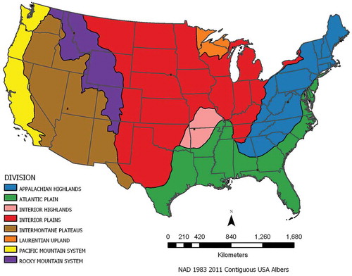
An effective method of comparing US Topo contours is to view them at the intersection of four quadrangles using background imagery of the legacy 7.5′ topography, which shows the legacy contours in a light gray. One set of four quadrangles was chosen for each of the physiographic divisions (Fenneman 1917). Two criteria were used when choosing quadrangles for analysis: quads containing differing source elevation data, and quads spanning state borders, where possible. The contours themselves were not viewed or considered in the selection of quads. In the following figures, contour depressions are displayed with red – instead of brown – lines to make them easier to detect.

In the Rocky Mountain System, source data for the southern quadrangles are DEMs from higher-resolution (lidar, in this case) elevation data (hereafter referred to as HR contours). In fact, the lidar project from which they were derived extends into the northern quads up to the state border. North of the border line, contours were produced from 10 m DEMs derived mainly by digitizing legacy contours (hereafter referred to as 10 m contours) (Figure 4). Note how closely the 10-m contours match legacy contours as compared to those derived from lidar. US Topo contours edge-match better than the legacy contours did. This is due to the small overlap used when creating contours, then clipping them back to the quadrangle boundary. In general, legacy contours and 10 m contours tend to look more simplified and smoother than HR contours (Figure 4 – compare (a) to (b)), although the number of vertices (relative to the cell size of the input data), which determines level of simplification, is the same for all US Topo contours. In steeper areas like the Rocky Mountain System, this results in a very different overall characteristic of the US Topo contours relative to legacy contours.

Figure 4. Comparison of US Topo contours at the intersection of four quadrangles in the Rocky Mountain System. Background imagery is the legacy 7.5’ topography (legacy contours are gray). Source data for the southern quadrangles are lidar-derived DEMs, while the northern quadrangles (north of bold black line) were produced from 10 meter DEMs derived from digitized legacy contours.

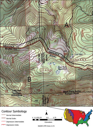
ASCEND’s NHD high-resolution water body treatment can be quite effective at integrating elevation and hydrography, especially in simple hydrological terrain (Figure 5). In the Ranger Peak quadrangle of Idaho the US Topo contours (lidar-based) only vaguely resemble the legacy contours.

Figure 5. Contour water body treatment in the Rocky Mountain System, Ranger Peak quadrangle (lidar source data). Background imagery is the legacy 7.5’ topography. NHD high-resolution Water body treatment of simple structures is quite effective within the same quadrangle. US Topo and legacy contours differ quite obviously here.

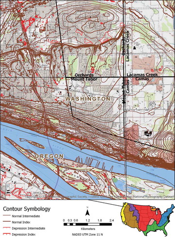
In the Pacific Mountain System, source data for the southern quadrangles are lidar-derived DEMs, while the northern quadrangles were produced from both lidar and 10 m DEMs, particularly in the north eastern quadrant (Figure 6). The area is marked by numerous depressions and greater detail, particularly in the HR contours, even though the source data for all quads is the same resolution. The “artistic” representation of terrain on the legacy quads is mirrored by the contours created from the 10-m DEMs.

Figure 6. Comparison of US Topo contours at the intersection of four quadrangles in the Pacific Mountain System. Background imagery is the legacy 7.5’ topography (legacy contours are gray). Source data for the area west and south of the bold black line are lidar-derived DEMs, while the contours inside the bold black lines were produced from both lidar and 10 meter DEMs.

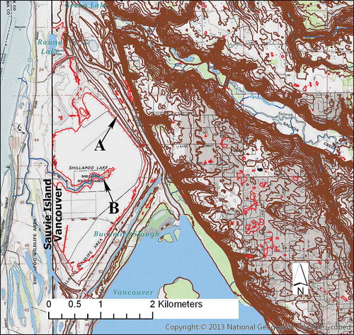
Complex elevation and water features along the Columbia River in the Pacific Mountain System create interesting challenges (Figure 7). Lidar source data in the Vancouver quadrangle result in overly intricate and coalesced contours. Although Shillapoo Lake, seen in the legacy quadrangle, has disappeared from the NHD, a depression of the same size and shape signifies the location (Figure 7(a)). A new stream, burned into the lake bed by ANDUDEM, complicates the contours even further (Figure 7(b)).

Figure 7. Representation of complex elevation and water features along the Columbia River in the Pacific Mountain System. Lidar source data in the Vancouver quadrangle result in overly intricate and coalesced contours. Although Shillapoo Lake, seen in the legacy quadrangle, has disappeared from the NHD, a depression of the same size and shape signifies the location (A). A new stream, burned into the lake bed by ANDUDEM, complicates the contours even further (B).

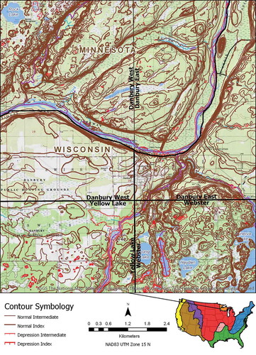
In the Laurentian Upland, US Topo HR contours represent glacial terrain more accurately than legacy or 10 m contours (Figure 8). Again, note the generally smoother appearance of the 10 m contours.

Figure 8. Comparison of US Topo contours at the intersection of four quadrangles in the Laurentian Upland. Background imagery is the legacy 7.5’ topography. Source data for the quadrangles north of the bold black line are lidar-derived DEMs, while the southern quadrangles and the southern portion of the northern quadrangles were produced from 10 meter DEMs derived from digitized legacy contours.

In the Black Lake quadrangle of the Laurentian Upland, HR contours depict subtleties in the terrain not depicted in the legacy contours. Small depressions opposite a stream along a railroad grade are not only represented in the higher resolution elevation data, they were saved by the automated routine that deletes tops and depressions below the desired threshold (Figure 9(a)). The legacy map is missing these depressions and the contour along the stream channel extends further upstream, possibly due to an inability of the compiler to precisely resolve the ground in the original stereo imagery, vertical accuracy differences between elevation collection technologies, or ground subsidence over time (Figure 9(b)).

Figure 9. High-resolution contours depict subtleties in the terrain not depicted in the legacy contours. Small depressions are not only represented in the higher resolution elevation data, they were saved by the automated routine that deletes tops and depressions below the desired threshold (A). The same contours are missing from the legacy map (B).

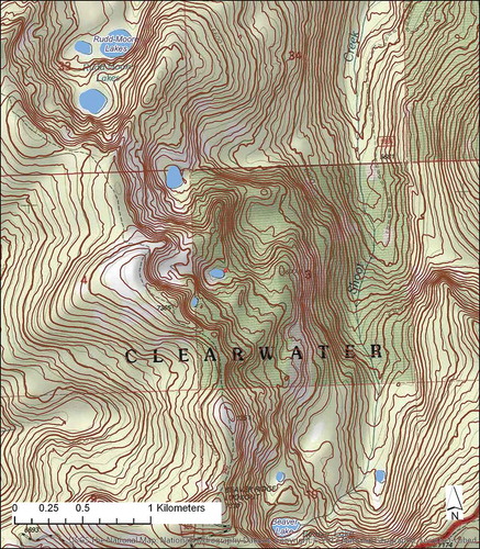
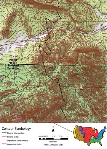
In the Intermontane Plateaus, HR contours appear more chaotic and less uniform than do the 10-m contours (Figure 10). The irregular contours correctly give the impression of a more chaotic terrain, particularly north of Leach Canyon. HR contours are less uniform and rounded, more accurately representing the terrain than legacy contours created with human cartographic license. Note that Kanarraville has a larger contour interval than the other three quadrangles.

Figure 10. Comparison of US Topo contours at the intersection of four quadrangles in the Intermontane Plateaus in Utah. Background imagery is the legacy 7.5’ topography. Source data for the eastern quadrangles are lidar-derived DEMs, while the western quadrangles west of the black line were produced from 10 meter DEMs derived from digitized legacy contours.

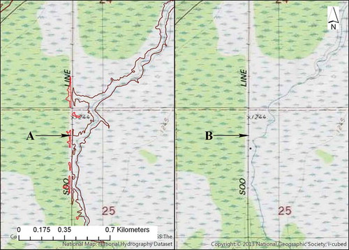
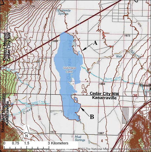
Quichipa Lake displays challenges encountered during contour automation when water bodies cross quad boundaries of Cedar City NW and Kanarraville, UT in the Intermontane Plateaus (Figure 11). The elevation data are more current and accurate than the hydrography data, resulting in unsatisfactory contour representation of the terrain. The contour at Figure 11(a) is missing from the southern quadrangle due to change in contour interval. However, the contour at Figure 11(b) fails to appear opposite the border because elevation data were collected at a lower lake level. The matching contour was created inside the water body, and hence was subsequently removed by ASCEND.

Figure 11. Contour automation is challenging where elevation and hydrography data integrate poorly along the Cedar City NW and Kanarraville quadrangles in Utah. The elevation data are more current and accurate than the hydrography data, resulting in unsatisfactory contour representation of the terrain. The contour at A is missing from the southern quadrangle due to change in contour interval. However, the contour at B fails to appear opposite the border because elevation data were collected at a lower lake level. The matching contour was created inside the water body, and hence was subsequently removed by ASCEND.

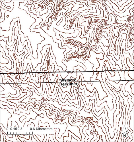
In the Interior Plains, the less uniform contours from lidar (south of bold black line) provide a more accurate depiction of the true landscape than the generalized human-drawn contours (north) (Figure 12).

Figure 12. Comparison of US Topo contours at the intersection of four quadrangles in the Interior Plains. Source data for the quadrangles south of the bold black line are lidar-derived DEMs, while contours north of the bold black line were produced from 10 meter DEMs derived from digitized legacy contours.

A larger scale view of the area demonstrates how well ASCEND algorithms can, in this case, produce contours to match the legacy or 10-m contours (Figure 13). In fact, it would be almost impossible to discern the line between the differing data sources.

Figure 13. ASCEND algorithms can – as in this case – produce contours that match the 10-m contours (south of bold black line) quite well.

The Interior Highlands demonstrate how well ASCEND can represents contours along water bodies even at the intersection of four quadrangles (Figure 14). Recall that each quadrangle is generated separately, and at state boundaries may even be run at different times, in different states, with different versions of the software. Note here how closely the HR contours (west of bold black line) resemble the 10-m contours (east).

Figure 14. Comparison of US Topo contours at the intersection of four quadrangles in the Interior Highlands. Background imagery is the legacy 7.5’ topography. Source data for the western quadrangles, and the western part of the eastern quadrangles are lidar-derived DEMs, while the eastern sides of the eastern quadrangles were produced from 10 meter DEMs derived from digitization of legacy contours.

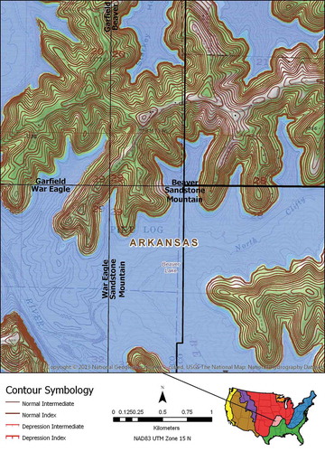
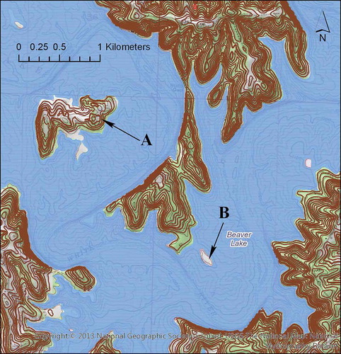
Contours on big islands are handled correctly by the software (Figure 15(a)), but sometimes the software fails to produce contours on small islands (Figure 15(b)). This is due to misalignment between the hydrography and elevation data.

Figure 15. Contours on big islands in the War Eagle quadrangle are handled correctly by ASCEND (A), but sometimes the software fails to produce contours on small islands due to hydrography and elevation misalignment (B). The contour seen in B exists in the legacy Topo, but ASCEND did not create a contour in the same position due to the encroachment of the lake. Contours seen below the water are bathymetry contours from the legacy quadrangle.

Most of the northern quadrangle contours (north of the bold black line) in Atlantic Plain swampland derive from 10 m source data, and here depressions are much less frequent than in the southern quadrangles derived from lidar (Figure 16). More depressions were likely introduced by the higher resolution data.

Figure 16. Comparison of US Topo contours at the intersection of four quadrangles in the Atlantic Plain. Background imagery is the legacy 7.5’ topography. Source data for the southern quadrangles and the southern part of the northern quadrangles are lidar-derived DEMs, while the northern quadrangles north of the bold black line were produced from 10 meter DEMs derived from digitized legacy contours.

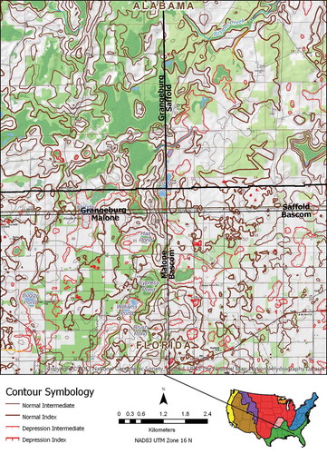
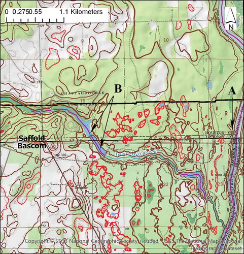
Contours along the borders of the Saffold and Bascom quadrangles display elevation and hydrography interactions in complex terrain. The Chatahoochee River is a double-line stream in the NHD, which is connected to the network via an artificial path (purple line) (Figure 17(a)). Irwin Mill Creek is a perennial stream along the turquoise line but is represented as small lakes in certain places, which are also connected to the network via artificial paths (Figure 17(b)).

Figure 17. Contours along the borders of the Saffold and Bascom quadrangles display elevation and hydrography interactions in complex terrain. The Chattahoochee River is a double-line stream in the NHD, which is connected to the network via an artificial path (purple line) (A). Irwin Mill Creek is a perennial stream along the turquoise line, but is represented as small lakes in certain places, which are also connected to the network via artificial paths (B).

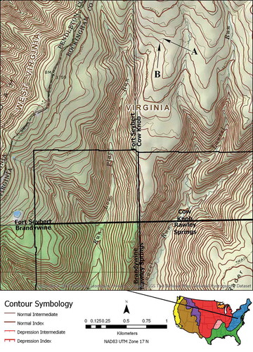
In the Cow Knob quad of the Appalachian Highlands, rugged terrain demonstrates a drawback to automating contours for the nation, where the smoothing of the elevation data required to reduce noise in very steep terrains leaves contours in flatter areas less detailed than desired (Figure 18). Compare the legacy contours (Figure 18(a)) to their US Topo lidar-derived counterparts (Figure 18(b)). The smoothness is controlled by a parameter that can be varied from one quadrangle to next, but not within one. This smoothing is not an issue in the 10 m data, as the contours are based on a degree of line work generalization chosen by the original cartographer. Decreasing the smoothness of the lidar-derived contours would likely have resulted in contours more similar to the legacy contours.

Figure 18. Comparison of US Topo contours at the intersection of four quadrangles in the Appalachian Highlands. Background imagery is the legacy 7.5’ topography. Rawley Springs and adjoining portions of the other three quadrangles (inside bold black lines) were produced from 10 meter DEMs derived from digitized legacy contours, while the source data for the remaining contours are lidar-derived DEMs.

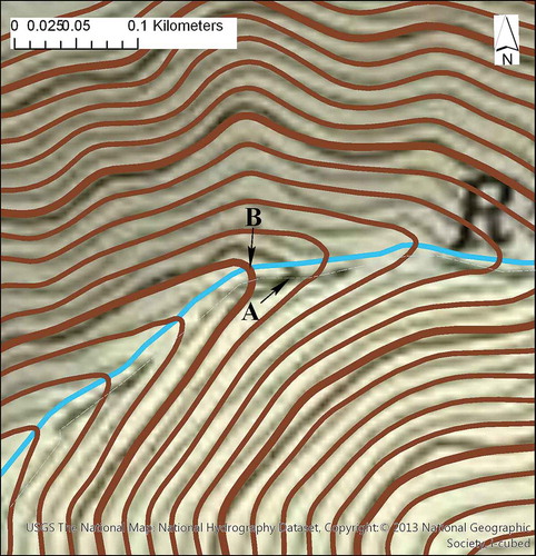
Often the biggest differences between legacy and US Topo contours, despite data source resolution, fall along NHD Flowlines, where they have been burned into the DEM. Although in some cases this may result from the parameters used in ANUDEM, typically it is due to changes in the Flowlines themselves as stored in the NHD. Change in stream locations, and realignment of contours are clearly shown in the Cow Knob quadrangle of the Appalachian Highlands (Figure 19). Such a change results in the difference in location between the legacy contour at Figure 19(a), as compared to the realigned US Topo contour at Figure 19(b). The difference in US Topo contours relative to the legacy contours in the area that lies North – Northeast from A to B is due to the smoothing of the surface required to effectively burn the stream into the DEM surface.

Figure 19. Realignment of US Topo contours along updated NHD flowlines (streams) in the Cow Knob quadrangle of the Appalachian highlands. Note the difference in location between the legacy stream and contour at (A), as compared to the realigned stream (turquoise line) and US Topo contour at (B).

One challenge in automating contour production that occurs often enough to be a concern, namely: stream trenching from inverted stream gradients, was not represented in any of the randomly selected areas. In order to demonstrate this challenge, a quad containing examples of this issue was sought and found in the Interior Plains. In the Bristol quadrangle in northeastern Indiana, contours incorrectly enclose a stream instead of turning back along it (Figure 20(a)). This phenomenon is caused by NHD flowlines that are inverted relative to the surrounding terrain either because their flow direction is wrong, or the spatial alignment between the elevation and hydrography fails to agree. ANUDEM burns in these streams based on the from–to nodes, which results in contours following the stream instead of crossing it. This happens more frequently when the source data are lidar as is the case for this quadrangle. To correct this problem, the NHD direction-of-flow is either manually flipped, as in this case, or removed altogether, and then the quadrangle is reprocessed through ASCEND (Figure 21). Major general successes in automating contour production for CONUS include water body treatment in simpler terrain, turnback realignment, and simplification and presentation of the US Topo contours. Challenges to automation include representing terrain at the same degree of smoothness throughout CONUS, complex terrain/NHD feature interaction, poor spatial alignment between elevation and hydrography data, and HR source data artifacts.

Figure 20. Contours sweeping around NHD flowlines instead of crossing them in inverted stream gradients (A) in the Bristol, IN quadrangle present challenges to automation of contours for the entire U.S., but especially when the source data are lidar, as is the case for this quadrangle.

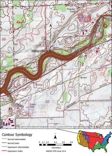
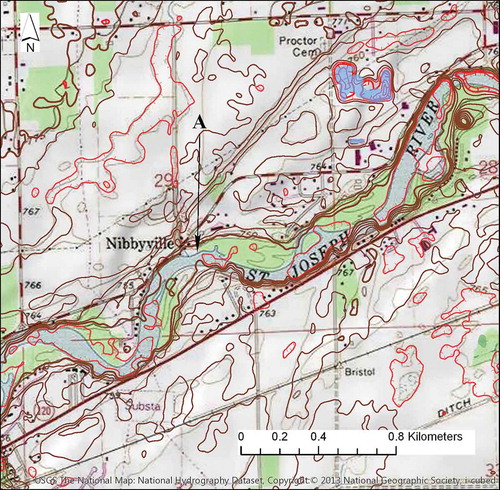
Figure 21. Corrected contours (A) after the inverted NHD Flowline direction was flipped, and the quadrangle was reprocessed by ASCEND.

Conclusion

Developing an automation package to produce contours for over 54,000 7.5′ topographic quadrangles for the CONUS has been a tremendous – yet rewarding – challenge. Great diversity in US terrain and in-source characteristics of national hydrographic and elevation data sets lead to complex and variable interactions between water features and contours that in reality could benefit from differing algorithms from one geographic region to the next. Clearly, much more research is warranted in this direction than was available in preparation for the US Topo program.

Undoubtedly, better alignment of the elevation and hydrography data would improve output from automated generation of contours. Improving the positional registration of corresponding features between these data sets is the goal of an ongoing USGS project referred to as Elehydro.

ASCEND has numerous parameters whose effect on contours has remained unexplored due to time constraints. Experimentation with these parameters would likely lead to improved positional integration of these two categories of US Topo features. For example, the water body leveling statistic sacrifices robustness in attempt to circumvent issues with other flattening processes by averaging the MAD with the IQD, the output of which is more affected by incorrect values. Instead of calculating the average of the two, it may make sense to start with the MAD and fall back on the IQD should the former reduce to zero. Another option would be to impose a minimum based on a tolerance relative to the median. Additional alternatives may also be considered.

The user community will need time to adjust to the less uniform, less rounded and more jagged contours generated directly from high-resolution elevation data, as compared to the legacy contours that were carefully hand-crafted by an army of cartographers to enhance topographic expression. However, it is important to consider that this new appearance is not flawed, but merely different. In fact, it is a more accurate representation of the true subtleties of the national terrain.

Acknowledgments

We would like to acknowledge the input from anonymous reviewers whose feedback helped to greatly improve the paper. This work was supported by the staff of the National Geospatial Technical Operations Center of the U.S. Geological Survey.

Disclosure statement

No potential conflict of interest was reported by the authors.

References

- Arundel, S. T., L. A. Phillips, A. J. Lowe, J. Bobinmyer, K. S. Mantey, C. A. Dunn, E. W. Constance, and E. L. Usery. 2015. “Preparing The National Map for the 3D Elevation Program – Products, Process and Research.” Cartography and Geographic Information Science 42 (sup1): 40–53. doi:10.1080/15230406.2015.1057229.
- Bodansky, E., A. Gribov, and M. Pilouk. 2002. “Smoothing and Compression of Lines Obtained by Raster-to-Vector; Conversion.” In Graphics Recognition: Algorithms and Applications, edited by Dorothea Blostein and Young-Bin Kwon, 256–265. Heidelberg: Springer. doi:10.1007/3-540-45868-9_22.
- Douglas, D., and T. Peucker. 1973. “Algorithms for the Reduction of the Number of Points Required to Represent a Digitized Line or Its Caricature.” The Canadian Cartographer 10 (2): 112–122. doi:10.3138/FM57-6770-U75U-7727.
- Evans, R. T., and H. M. Frye. 2009. History of the Topographic Branch (Division). (Circular 1341) Reston, VA: U.S. Geological Survey.
- Fenneman, N. M. 1917. “Physiographic Subdivision of the United States.” Proceedings of the National Academy of Sciences of the United States of America 3: 17–22. doi:10.1073/pnas.3.1.17.
- Gesch, D. B. (U.S. Geological Survey). 2007. “The National Elevation Dataset.” In Digital Elevation Model Technologies and Applications: The DEM Users Manual, edited by D. Maune, 99–118. 2nd ed. Bethesda, MD: American Society of Photogrammetry and Remote Sensing.
- Huber, P. J., and E. M. Ronchetti. 2009. Robust Statistics. Hoboken, NJ: Wiley.
- Hutchinson, M. F. 1989. “A New Procedure for Gridding Elevation and Stream Line Data with Automatic Removal of Spurious Pits.” Journal of Hydrology 106 (3–4): 211–232. doi:10.1016/0022-1694(89)90073-5.
- Hutchinson, M. F. 2000. “Optimising the Degree of Data Smoothing for Locally Adaptive Finite Element Bivariate Smoothing Splines.” ANZIAM Journal 42: 774–796. doi:10.21914/anziamj.v42i0.621.
- Hutchinson, M. F. 2007. ANUDEM. Canberra: Australian National University.
- Hutchinson, M. F. 2008. “Adding the Z-Dimension.” In Handbook of Geographic Information Science, edited by J. P. Wilson and A. S. Fotheringham, 144–168. Malden, MA: Blackwell.
- Hutchinson, M. F. 2011. ANUDEM Version 5.3 User Guide. Canberra: CRES 2006.
- U.S. Geological Survey. 2003. “Part 7–Hypsography,Standards for USGS and USDA Forest Service Single Edition Quadrangle Maps. Draft for Implementation.” [map]. Primary Series Quadrangle Map Standards, U.S. Geological Survey. http://nationalmap.gov/standards/qmapstds.html