Motion of animated streamlets appears to surpass their graphical alterations in human visual detection of vector field maxima

ABSTRACT

Animations have become a frequently utilized illustration technique on maps but changes in their graphical loading remain understudied in empirical geovisualization and cartographic research. Animated streamlets have gained attention as an illustrative animation technique and have become popular on widely viewed maps. We conducted an experiment to investigate how altering four major animation parameters of animated streamlets affects people’s reading performance of field maxima on vector fields. The study involved 73 participants who performed reaction-time tasks on pointing maxima on vector field stimuli. Reaction times and correctness of answers changed surprisingly little between visually different animations, with only a few occasional statistical significances. The results suggest that motion of animated streamlets is such a strong visual cue that altering graphical parameters makes only little difference when searching for the maxima. This leads to the conclusion that, for this kind of a task, animated streamlets on maps can be designed relatively freely in graphical terms and their style fitted to other contents of the map. In the broader visual and geovisual analytics context, the results can lead to more generally hypothesizing that graphical loading of animations with continuous motion flux could be altered without severely affecting their communicative power.

KEYWORDS:

• Animation
• streamlet
• graphical loading
• vector field
• map
• experiment
• visual search

1. Introduction

Animation has become a ubiquitous illustration technique in cartography as well as in visual (e.g. Thomas & Cook, 2006) and geovisual analytics (e.g. Keim et al., 2008; Teufert, 2004). Animation is typically used for illustrating spatio-temporal phenomena, such as moving objects (e.g. Maggi, Fabrikant, Imbert, & Hurter, 2016) and environmental events (e.g. Saint-Marc, Villanova-Oliver, Davoine, Capoccioni, & Chenier, 2017), and sometimes also non-temporal spatial phenomena (Peterson, 1996). Despite the omnipresence of animation in people’s current everyday lives, the quality of many geospatial animations remains low in readability, interpretability, and informational efficiency because thorough golden practices and design principles have not yet been established if created at all, and, even less, taken in use. Compared to the design principles of traditional geovisualization, mostly developed through centuries by cartographic work (see Bertin, 1967; Imhof, 1965; MacEachren, 1995), principles of designing geospatial animations still seem to be on their initial steps in spite of having been a topic in research literature for decades (Campbell & Egbert, 1990; Resch, Hillen, Reimer, & Spitzer, 2013). This slow evolution of design may be due to the facts that (1) animation is technically more complicated to produce, which leads to the need to control a higher number of visualization parameters, and (2) animations are cognitively much more challenging for people to read than static images (Harrower, 2007), which requires more careful design in order to ensure the transfer of the desired information. Moreover, appropriate use cases for animation can be challenging to identify, and trying to apply animation for inappropriate cases may lead to focusing on misleading factors of design (e.g. Lowe, 2003, 2004).

A common task in visual analytics is looking for patterns in massive spatio-temporal data (e.g. Keim et al., 2008; Maciejewski et al., 2010). Seeking for patterns may be focused on objects alone or on the movement of objects (e.g. Ferreira, Poco, Vo, Freire, & Silva, 2013; Willems, Van De Wetering, & Van Wijk, 2009). It can also concentrate on more complicated spatial reasoning tasks with goals not directly related to objects themselves but rather to their impact on the behavior of some other object or phenomenon (Pyysalo & Oksanen, 2013). The article of Pyysalo and Oksanen described a concept of a three-layer situational awareness map: in the visual hierarchy, the background map was at the bottom, the topical thematic layer on the top, and between them was a supporting middle layer that facilitated spatial reasoning about the thematic layer. The present study is based on the idea of making the supporting middle layer animated, which can be expected to support spatial reasoning.

In order to get more empirical grip on how the appearance of animations on geovisualizations and maps may affect human reading, we conducted an empirical reaction-time study with search tasks on two-dimensional geovisualizations of vector fields. We visualized vector fields using animated streamlets that are gradually disappearing line particles along streamlines of a vector field. We chose this type of animation for our study of parameter changes because animated streamlets have been previously evaluated as the most communicative form among the common animation methods of vector fields (Ware, Bolan, Miller, Rogers, & Ahrens, 2016). Animated streamlets have also become commonly used in popular vector field visualizations, such as weather maps on TV and video channels, which makes understanding their use of foremost interest. We implemented our animations using one of the earliest comprehensive applications of animated streamlets for wind maps by Viégas and Wattenberg (2012), that is widely recognized for its high visual and cartographic quality.

The exact research question of the study was to determine how the appearance of animated streamlets affects performance in visual search tasks of maxima on two-dimensional vector fields. An explorative aim was to study the usage of different kinds of animation parameters in a visual analytics context, and to contribute to the gradually enlargening set of guidelines for creating more user-friendly geospatial animations for geovisual analytics and beyond.

This article continues with a literature review of geospatial animation in general and in cases of vector fields similar to our study in Section 2. Section 3 introduces the experimental setup of the study in terms of design, techniques, participants, and analytical methods. Section 4 introduces the results of the experiments with initial analyses, and Section 5 discusses the results as they relate to previous knowledge as well as shortcomings and generalizability of the study. Lastly, Section 6 concludes the presented study and looks at necessary future research on cartographic animation.

2. Related research

The history of animation dates back to the first half of the nineteenth century, but geospatial animation emerged only a century later on maps in movies of 1930s and 40s (Campbell & Egbert, 1990). Since then, geospatial animation in cartography was used and studied on a steady but relatively quiescent pace until the appearance of the personal computer, which launched a new era for geospatial animation in the 1990s (e.g. Campbell & Egbert, 1990; DiBiase, MacEachren, Krygier, & Reeves, 1992; Dorling, 1992; Koussoulakou & Kraak, 1992). In the new millennium, visual and geovisual analytics quickly emerged with a novel perspective on visualization, taking animation as a central means of dynamic geovisual representation (Thomas & Cook, 2006). The volume of visual analytic and geospatial animations has had an immense growth since then and animation design issues have been considered widely in geovisual analytics and cartographic literature (e.g. Castronovo, Chui, & Naumova, 2009; Harrower, 2007; Harrower & Fabrikant, 2008; Resch et al., 2013; Shipley, Fabrikant, & Lautenschütz, 2013). However, empirical research on quality and usability of animated graphics in geovisualization has been much less intense. In the following paragraphs, we present a few experiments that provide some empirical evidence on the usability of animation in visualizing geodata.

With regard to usefulness of geospatial animation from the cartographic viewpoint, animated maps have been widely debated in literature in contrast to static small-multiple maps, and several comparative usability experiments have been conducted. Qualitative evidence in the form of questionnaires, interviews, and group discussions about animation experiments supports the superiority of animation for overviews of spatio-temporal phenomena (Boyandin, Bertini, & Lalanne, 2012; Koussoulakou & Kraak, 1992; Slocum, Sluter, Kessler, & Yoder, 2004). Some quantitative evidence shows animation allowing for faster and more accurate observation of spatio-temporal phenomena and enabling the perception of motion, unlike small-multiple maps (Griffin, MacEachren, Hardisty, Steiner, & Li, 2006). The very same and other studies also provide evidence on small-multiples to be favorable over animation for comparing distant moments of time because people cannot easily hold separate moments in their long-term memory, whereas small-multiples allow for visual comparison of those moments directly (Boyandin et al., 2012; Fabrikant, Rebich-Hespanha, Andrienko, Andrienko, & Montello, 2008; Slocum et al., 2004). The results of unfavorable use cases of animation also appear in these studies, often related to insufficient sets of interactive tools (e.g. Boyandin et al., 2012; Cinnamon et al., 2009; Slocum et al., 2004). All the studies conclude about the need of careful design of animations for the desired purpose.

The challenging nature of designing and reading animations has been distinctively illustrated by the experiments of Lowe (2003, 2004), who studied animation as a means of conveying geospatial education and used complex interactive weather maps as his stimuli. His experiment with novice students in meteorology shows that untrained people tend to focus on local and visually appealing features rather than look at the whole of the map or concentrate on features with high substantial relevance. These results reflect (1) the problem of split attention on animations, which occurs when the viewer should follow multiple spatially separate features simultaneously, inconveniently with his or her processing capabilities (Mayer, 2002) and (2) the visuo-perceptive process of focusing reflexively on salient features when high-level mental models for interpreting a complex visualization do not exist (Mayer, Dorflinger, Rao, & Seidenberg, 2004). According to this experiment, changes in position provide for the most salient visual cues in animation, whereas changes in form are not easily recognized. Lowe concludes by stating that animations for novices should be designed with proactive indication of substantially central content and cases of split attention should be avoided.

Vector fields have been a compelling target for animation due to their spatial ubiquity that enforces the animator to use a symbolized representation of a continuous field, and due to common appearance of vector fields in nature and techniques, such as flows of water, air, and electro-magnetism. The development of flow field visualization in computer graphics has led to the creation of animation techniques like dynamic arrows as pathlets or streamlets (see Jobard, Ray, & Sokolov, 2012), animated orthogonal particles, and animated streamlets (see Ware et al., 2016). Ware et al. (2016) carried out two usability experiments on the effectiveness of the last two animation methods against two more traditional static representation methods, measuring both accuracy of flow pattern recognition and reaction times in a task of flow tracking. Their results rated animated streamlets the most effective representation of the attempted ones in both tasks, followed by static equally spaced streamlines, animated orthogonal particles and last, the traditionally frequently used static arrow grid.

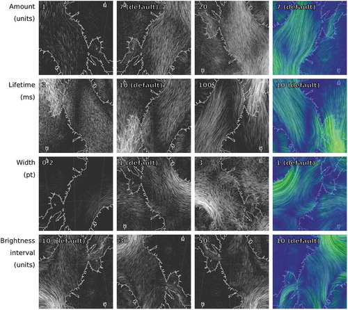
Animated streamlets are line particles that move along streamlines of a vector field and indicate the local strength and direction of the field by their graphical style of animation. When high numbers of these line particles are systematically placed on a vector field, an effective visualization of the structure of the field occurs (see Figure 1). In the animation solution of Viégas and Wattenberg (2012), strength of a vector field is illustrated by velocity, brightness, and color of the animated streamlets.

Figure 1. Static frames of the animated stimuli in the search tasks of the experiment. Increasing the “Brightness interval” causes visible borders between the strengths of the vector field. Animated stimuli are visible as supplemental material in the Figshare web service.

In our literature review, we have not become aware of previous empirical experiments about the effects of changing graphical appearance of vector field animations. This seems to be a gap in the previous research (e.g. Shipley et al., 2013), which we begin to fill with the study presented in this article.

3. Materials and methods

The empirical experiment of the study was carefully designed according to the exact research question of the study. We piloted the experiment with $10$ participants in a laboratory environment before proceeding to the actual experiment that grew to include a total of $73$ new participants in laboratory and web environments. The pilot experiment indicated several weaknesses in the original design, so we enhanced the design for the actual experiment. For example, new clearly single-maximum wind fields were selected as stimuli in order to minimize ambiguousness while responding and a new geographical region was chosen that was more difficult to recognize.

For the actual experiment, laboratory sessions were conducted first. Observations by an experimenter revealed some difficulty in the interpretation of the task assignments and lead to ignoring several tasks from analysis. Therefore, task assignments were clarified and challenging parts were highlighted in the textual instructions in order to avoid faulty performance as much as possible. The substantial content of the task assignments did not change.

3.1. Participants

A total of $73$ persons took part in the experiment, of whom $32$ were in the laboratory and $41$ were in the web environment. Laboratory participants were employees of the National Land Survey of Finland and web participants were invited through email lists of geoinformatic, cartographic and visualization research and development communities (Table 1). Hence, participants can be considered technologically skillful and reliable experimentees.

Table 1. Background information of the participants.

Email lists	AGILE 2016 Code Loves Maps workshop
(call for participation)	International Cartographic Association, Commission on GeoVisualization,
	Finnish Lynet visualization workshop
	Cartographic Society of Finland
Total number of participants	$73$
Age (min–median–max)	$24$–$34$–$72$
Women: Men	$43$: $30$
Wind field experience	$1$
Glasses	$40$
Vision disorder	$3$

Collected background information of the participants are listed in Table 1. One self-reported indication of experience on wind fields and the three vision disorders were such that they did not affect the performance in the experiment.

3.2. Software, conditions, and stimuli

The experimental procedure was programmed in the Tatool Web software for online experiments (von Bastian, Locher, & Ruflin, 2013), which allowed for running the experiment both in laboratory and web environments. Instances of Tatool Web were installed on a laptop for laboratory sessions and on a cloud server for web sessions. In the laboratory, an external mouse was used and an experimenter guided the sessions. The experimenter was available for the participants but only briefly answered to their possible questions after the initial guidance was given. In the web sessions, participants were instructed to use only external mice and keyboards and to avoid touch devices.

The map animation stimuli were created using the earth web software that renders static vector fields in a web browser on a virtual globe using transparent, gradually disappearing animated streamlets (see http://earth.nullschool.net). The software and wind data were installed on a local server on a laptop and screen recordings were taken and processed to finished videos for the experiment. Animation stimuli were created that depict static vector fields of wind ($10$ s, $350$ x $350$ px, see Figure 1).

The wind data for the animation stimuli were from the Global Forecast System of the NOAA. The coastline data on the animations was from Natural Earth. In addition, a lightly rendered geographical grid with latitudes and longitudes was present in the animations. All these data are rendered by the earth software by default.

Wind fields for the stimuli were selected so that single areas of correct answers were easily identifiable. Four unique wind fields were acquired for each of the studied four animation parameters. Geographical regions for the stimuli were chosen remote and difficult to recognize for expected participants so that recognizing the area would not occur and affect the performance of the tasks. The region of the Labrador Sea was chosen due to its remote location, sparse population, and expectedly low awareness of participants about the area. We asked participants of the pilot study if they recognized the region and got only responses in the negative. In addition, stimuli were flipped between tasks for preventing recognition of the region.

3.3. Experimental design

The experiment was designed for studying the effects of animation parameters of animated streamlets as independent variables. Four parameters were studied: (1) the amount of streamlets (or density); (2) the lifetime of a streamlet (or length); (3) the width of a streamlet; and (4) the brightness interval in streamlets that may cause visual isoline borders denoting the intensity levels of the field (or the strength of posterization).

Graphically distinct low, medium, and high values of each parameter were selected and rendered in gray-scale animations so that trends in dependent variables along value ranges would be observable. In order to study the effect of color in animations, a colored version of each wind field was included in the trials, in which color hue represented the wind speed. Hence, the experiment contained $16$ map animation stimuli in total for the actual trials (see Figure 1). The selected parameter values contain default values of the earth software. Default parameter values were also utilized in the colored animations.

We tested two typical kinds of tasks in the experiment that require careful observation of the strength of a vector field: (1) finding the area of highest intensity (animation-only search) and (2) finding the area of highest intensity on a coastline (animation-static search). For these tasks, two dependent variables were measured: reaction time and correctness of answer. The correct answer for the area of highest intensity was defined as pointing at any location inside an area of highest intensity level as seen in the animation with the high brightness interval $50$, extended by a pointing inaccuracy buffer of $15$ pixels (Figure 2). For the area of highest intensity on a line, the same level of highest intensity was cut with buffers of $15$ pixels out of lines in order to define the correct answer (Figure 2). Both of the search tasks were primed by training trials with three separate animation stimuli from a different region than in the actual trials, in order to get the participants accustomed to the task and to perform at their true performance level in all actual trials.

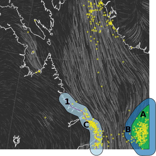
Figure 2. Answers to and areas of correct answer for the “amount of streamlets” stimuli (visualized here using the high value “50” of “brightness interval”). Area A: Area of highest intensity level. Area B: Area of correct answer for animation-only search (with the pointing inaccuracy buffer of $15$ px). Line 1: Coastline with the strongest wind. Area C: Area of correct answer for animation-static search (with the inaccuracy buffer of $15$ px). Dots: All answers of the participants to the “amount of streamlets” stimuli.

In addition to actual animation tasks, a background questionnaire was included in the experiment in order to collect information about demographic control variables of the experiment: age, gender, experience with wind fields, use of glasses, and personal vision disorders. We chose these control variables because of their standard inclusion in usability studies (age, gender, experience on topic) and possible physical effects due to viewing conditions (glasses, personal vision disorders).

3.4. Procedure

The experimental session began with an introduction to the experiment that was given orally by the experimenter in the laboratory and as a written description online. Particularly, external mouse and keyboard were advised to be used, and the experiment was advised to be performed only once. The textual introduction as well as the consequent instructions are visible in Supplemental Materials. Each instruction mentioned that returning back to earlier parts of the experiment will not be possible.

Next, background info was collected through the background questionnaire.

Subsequently, the substantial tasks followed (see also Figure 3):

Figure 3. Procedure of the experiment.

(1) Training of either animation-only or animation-static search ($3$ animations);

(2) Either animation-only or animation-static search ($16$ animations: $4$ parameters × ($3$ values + color)):

● restricted random order: same wind field ($3$ values + color) not consecutively;

● animation for each $3$ values + color mirrored differently; and

(3) Steps (1) and (2) anew with either animation-static or animation-only search depending on which one was not yet performed.

The order of the animation-only and animation-static search tasks was randomized in order to control for hypothesized performance differences caused by the order of tasks. Each training and task set was introduced separately with text instructions highlighting the differences from the other tasks and advice to focus on the current task. In the area-finding tasks, the participant was also instructed to move the cursor to a cross that appeared onscreen before each animation. This was to prevent faulty reaction times due to shorter or longer distances for moving the cursor.

3.5. Classification of correct answers

For analyzing the correctness of answers in animation-only and animation-static search tasks, areas of correct answers were digitized using the QGIS software (QGIS Development Team, 2018, Figure 2) on the animation screenshots with the parameter “brightness interval” at high value $50$, which causes visible static borderlines in the animation. The brightest area, or the coastline on the brightest area, was digitized and enlargened with a buffer of $15$ pixels in order to eliminate errors due to pointing inaccuracy (Figure 2). Human digitization was done in order to achieve the appropriate level of generalization for the border line. Response points from the experimental sessions were then classified to be correct with QGIS if they resided inside the areas of correct answers.

3.6. Statistical analyses

We ran statistical analyses using the R software (R Core Team, 2018). Shapiro–Wilk tests and Q–Q plots indicated clearly non-normal distributions of reaction times, which led us to use non-parametrical statistics. For reaction-time analysis, we tested with the permutational multivariate ANOVA (PERMANOVA; Anderson, 2001) with $50,000$ iterations for each test. For subsequent pairwise tests, we used Wilcoxon rank sum tests with continuity correction and with the Holm method to correct for multiple testing.

For correctness of answers with multiple sample groups, we tested using a generalized linear model (GLM) with binomial logit link function and ran the pairwise tests using least-squares means (LS means) with Holm adjustment for multiple testing correction. Significance value of $p=0.05$ was used as a directive value for all statistical tests. With two sample groups, we used the test of equal proportions.

Statistical power analysis with power $0.8$ indicates small-to-medium effect size ($0.10<f<0.18$) for the omnibus tests of the experiment, which signifies high probability of finding even small effects in the data. For subsequent group-wise tests, the effect size indications are medium and above ($0.21<f<0.27$). For pairwise tests between sample groups, power analysis indicates medium-to-large effect sizes ($0.48<h<0.77$). These effect size indications serve well for answering the research questions of the current study.

4. Results

For the following results, $68$ animation-only and $56$ animation-static task performances were analyzed. Data on several search tasks was removed from the analyses due to faulty performance found in the data. In most of the faulty cases, participants performed the animation-static task without considering coastlines.

4.1. Reaction time

The omnibus PERMANOVA indicated clear statistically significant differences in reaction times between parameter values and color in the nested setting ($F=2.39$; $p=0.001$). In parameter-wise PERMANOVAs between parameter values and color, significant difference was indicated only for the parameter “amount of streamlets” ($F=3.59$; p =$0.003$): difference was found only between the low value $1$ and the colored animation in the animation-only search ($p=0.041$). In the animation-static search, two nearly significant differences were found between the low value $1$ and middle value $7$ ($p=0.085$) as well as the color ($p=0.063$). Reaction times were fastest for the colored animation and the default value $7$, and slowest for the low value $1$ and the high value $20$. Differences from the fastest to slowest median times were $1.01$–$1.88$ s (Figure 4).

Figure 4. Observations (circles) and medians (bold lines) of reaction times for the animation parameter “amount of streamlets” that was the only parameter for which value changes affected reaction times. One significant difference occurred between parameter values, depicted with normal and dashed lines.

Between vector fields with default parameter values (including colored animations), the omnibus PERMANOVA indicated clearly significant differences in reaction times ($F=17.54$, $p<0.001$). A pairwise Wilcoxon ranks sum test highlighted two cases of significant differences in levels of reaction times. Median reaction times with the vector field for the parameter “amount of streamlets” were $1.11$–$1.99$ s slower than with the other three fields ($p<0.001$), and reaction times with the vector field for the parameter “lifetime of a streamlet” were $0.65$–$0.88$ s slower than with that of “width of a streamlet” ($p<0.041$).

Between animations with and without color (default parameter values), significant differences in reaction times were not found ($p>0.12$).

4.2. Correctness of answers

The omnibus GLM analysis indicated differences in correctness of answers between parameter values and color in the nested setting (see Figure 5). For the animation-only search, contrasts of the least-square means indicated significantly low correctness for the high value “20” of the “amount of streamlets” compared to all other values (diff. of props. $>0.20$, $p<0.038$). For the animation-static search, significance was found for the high value “100” of the “lifetime” compared to the middle value “10” and the color (diff. of props. $>0.22$, $p<0.034$).

Figure 5. Correctness of answers among parameter values in search tasks. Orange highlight: parameters for which correctness varies significantly between values. (D) Denotes the default values of parameters (colored animations also had default values).

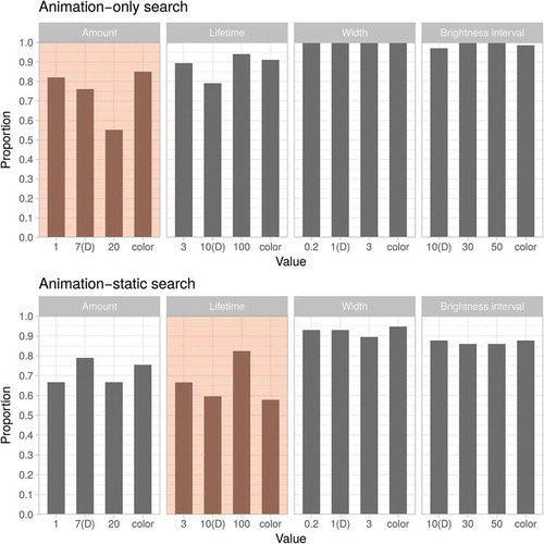
Between vector fields with default parameter values (including colored animations), the omnibus GLM analysis indicated clearly significant differences in correctness of answers ($p<0.05$). Both for the animation-only and animation-static search, contrasts of the least-square means highlighted differences between all of the vector fields ($p<0.001$) except “amount” and “lifetime” as well as “brightness interval” and “width.”

Use of color in animations did not affect the correctness of answers (compared to the default parameter values without color; $p>0.10$).

4.3. Effects of control variables

Experience on wind fields and vision disorder did not vary among participants (see Section 3.1). The omnibus PERMANOVA and GLM statistical analyses above indicated that reaction time was affected on clearly significant levels by all other control variables except age, and correctness of answers was affected by age and gender (Table 2). All effect sizes are noteworthy.

Table 2. Significant effects of control variables on dependent variables. RT: reaction time; A-only: animation-only search; A-S: animation-static search.

Control variable	Affected dependent variable(s)	Effect	Effect size	F or z	p
Email list	Reaction	Diff. of RT meds:	2.29 s	36.06	< 0.001
(call of part.)	time	max–min
Age	Correctness of answers	A-only coefficientA-S coefficient	−0.087 −0.12	−2.8 −5.2	0.005 < 0.001
Gender	Reaction	Diff. of RT meds:	1.10 s	22.77	< 0.001
	time	male–female
	Correctness	A-S diff. of props.	0.034	3.59	< 0.001
	of answers	male–female
Use of glasses	Reaction	Diff. of RT meds:	0.97 s	30.21	< 0.001
	time	no–yes
Order of	Reaction	Diff. of RT meds:	0.84 s	55.65	< 0.001
tasks	time	animation-static–
		animation-only

5. Discussion

5.1. Main findings

Changes in values of animation parameters' and using color affected participants’ responses surprisingly little. Statistically significant differences both in reaction times and correctness proportions were found in 3 out of 16 combinations of parameters and tasks, twice for the parameter “amount of streamlets” and once for the “lifetime of a streamlet.” Value changes of parameters “brightness interval” and “width of a streamlet” did not affect responses although they clearly change the visual appearance of the animation (see Figure 1).

No significant differences were found in reaction times between parameter values within non-colored animations (two instances that were nearly significances occurred). One significant difference was found in comparison to the colored animations, by the low value “1” of the parameter “amount of streamlets.” The visual difference between these two animations is clear but not particular compared to differences among other vector fields, which makes the difference appear occasional and insignificant for guiding the design of streamlet animations.

For the correctness of the answers, two significantly differing parameter values were found in different tasks. In the animation-only search, correctness proportions for the high value “20” of the parameter “amount of streamlets” were significantly lower than for the two other values and color. The corresponding animation is particularly dense and makes the global maximum difficult to recognize, which explains the observed significance. In the animation-static search, proportions for the high value “100” of “lifetime of a streamlet” were significantly higher than for one other value and color. This can be explained by the visual observation that long streamlets draw the form of the vector field in a more coherent and detailed manner. By our interpretation, these results can be taken as minor directive guidelines for the design of streamlet animations.

Overall, despite clear visual differences of animated vector fields between parameter values, changes in parameter values did not result in reaction time differences and resulted only in 3 differences (out of $24$) in correctness of answers due to 2 particular values (out of $10$ values). These results seem to suggest that there are no general tendencies over parameter value ranges that would affect the reading performance of the studied type of animations, but some particular choices of parameter values can occasionally make a difference in favor of more or less efficient viewing of the animation. Accuracy of reading seemed to be more prone to particular value choices than reading speed.

In addition, 1 significant difference in reaction times and 2 in correctness proportions (out of $12$ differences) were found in comparison to colored animations. Also for the use of color, the number of significances was minor although color contributed to slightly more differences than parameter values. There was no regular pattern for these differences either and the effects were both positive and negative, so the results cannot guide any design choices.

5.2. Limitations

Theoretically, the observed paucity of performance differences may be caused by the stimuli and tasks being so easy that differences do not emerge. We think that this is not the case in this study because each vector field in the stimuli contains several local maxima, which makes the tasks untrivial as answers must be carefully considered. Also, differences between parameter values are similarly absent for the easier animation-only and the harder animation-static search, even though between-task reaction times differ significantly.

However, different spatial structures of vector fields may play some role. Four of the total 6 found differences (and both of the close-to significances) occurred with the field for the parameter “amount of streamlets” that was also significantly the slowest one to respond in the experiment. Looking at Figure 1, unlike for the other fields, the global maximum of this particular vector field may have been ambiguous for the participants, which could cause the observed slower responses and weaker correctness of answers. Indeed, part of the answers were clustered around the other seemingly possible correct answer (see Figure 2). On the other hand, high correctness of answers for the parameters “width” and “brightness interval” may indicate clearer highest maxima in the corresponding vector fields. This observation of the varying quality among vector fields shows the importance of selecting maximally homogeneous stimuli for these kinds of visualization usability studies.

With regard to participants, we consider general representativeness of the experiment high because we analyzed results using differences on which the characteristics of the participating group has no or very little effect, particularly because the task was of a visuo-perceptional nature and did not require advanced abstraction of the actual spatial phenomena. The participants may have had somewhat advanced reading skills of geovisualizations on average, which may have made them faster and more accurate readers of the animation than average people, but the found paucity of performance differences should be present with any group of participants.

5.3. Controls

As for the control variables, five out of seven indicated some significant effect on participant performance. For email lists, high variance between lists was mostly due to some relatively homogeneous participant groups with short reaction times. Age decreased the correctness of answers, which was expected due to a well-known decrease of spatio-cognitive abilities by age (e.g. Ganguli et al., 2010). Slightly surprisingly, reaction times did not increase accordingly. Gender-wise, males responded importantly slower but with higher correctness in the harder animation-static searches than females. This could indicate higher focus on tasks by males although their on-average higher visuospatial abilities may also play a role (Halpern & Collaer, 2005). Use of glasses increased reaction time, which could be due to physical gestures like enhancing glasses. Order of tasks also affected reaction times, so that participants beginning with the more difficult animation-static search were slower overall. Possibly, doing the harder and more time-consuming task first made participants also concentrate harder and take more time on subsequent easier tasks. A similar effect was found earlier between the order of predictable (easier) and unpredictable (harder) letter discrimination tasks (Dreher, Koechlin, Ali, & Grafman, 2002). All of these control variables were included in the omnibus statistical tests so that their effects were accounted for in the analysis of dependent variables.

An important aspect to control in a within-subject study like this are the possible carry-over effects, in our case, learning of the task or stimuli that may make reaction times faster during an experimental session. The training task in our experimental procedure was to remove learning the task performance during a session, and flipping of vector fields as well as random order of animations was to remove carryover by stimuli. The number of trials per field and task ($4$) was too low to run statistical trend tests on the data, but visual review of observations and reaction-time graphs over trial sequences did not reveal any carry-over effects. We found only $5$–$8$ monotonically decreasing sequences of reactions times among $56$–$68$ reaction-time sequences for each of eight combinations of field and task, and even a few monotonically increasing sequences per field and task. In addition, when we asked our pilot participants about seeing same vector fields many times, almost all of them claimed not to have recognized the similarities between the fields. These observations seem to eliminate the possibility of carry-over effects being present.

5.4. Relevance

Previous research lacks empirical results on effects of changing visualization parameters of flux animations although suggestions and developments have been abundantly made about how to design animations based on, for example, cartographic principles (e.g. DiBiase et al., 1992), experimental software development (e.g. Jenny, Liem, Avri, & Putman, 2016), and empirical evaluations of animated applications (e.g. Maggi et al., 2016). Our study aimed to fill this gap in research and provide guidelines for choosing parameter values for animated streamlets. However, we ended up finding that continuous movement of animated streamlets is such a strong visual cue that choosing parameter values is mostly free of effects on reading performance when searching for maxima. We consider this finding relevant for geovisual animation design and research in weather as well as other applications with animated streamlets. The finding is also useful in directing further empirical research on animation parameters. A couple of particular parameter values that we found to affect task performance can lead animated streamlet design to use or avoid such values in some cases (see Section 5.1).

6. Conclusions

In the presented study, we found that altering values for major animated streamlet parameters, leading to clear visual influences on cartographic animation, does not affect reading performance of animation maxima in vector fields in any regular way. However, exceptionally, 2 occasional parameter values among a total of 10 values caused rare differences in participants’ performance. The results suggest that the parameter values of animated streamlets can be chosen quite freely with regard to the other contents of the map without losing visual information about the maxima in the field. For example, graphical loading of the animation can be made light in order to give more visibility to the underlying cartographic features, or strong in order to highlight the vector field itself. The value changes in parameters affected similarly little when the participants looked at the animation only or at the animation and static background coastlines simultaneously. In addition, the color field that visualized the strength of the vector field also had only occasional effects on the reading performance, indicating that color may be utilized for providing other information in the map view.

The conducted study contributes to building a foundation for design principles of animated maps, as wished by, for example, Shipley et al. (2013). This study also endorses the use of animated streamlets in supporting layers of multi-layered analytical geovisualizations (e.g. Pyysalo & Oksanen, 2013), as the graphical style of the streamlets can be quite freely fitted to other layers, at least when searching for maxima. Animated streamlet maps can be directly designed with the help of the gained knowledge since the strength of motion in the animation as a visual cue is clearly shown.

From a wider viewpoint of visual analytics, it can be hypothesized that the observed illustrativeness of continuous motion flux in animation is of some universal nature and that other kinds of such animations in also other kinds of tasks may follow some of the found freedom for choosing parameter values. This hypothesis calls for confirming and deeper-delving studies on the usability of different types of flux animations and with other kinds of experimental tasks, which could also feature additional measurements such as eye movement analysis (see Nossum, 2014).

Acknowledgments

The authors wish to acknowledge CSC – IT Center for Science, Finland, for server resources. Our most sincere thanks go to each and every experimentee. We are grateful to the anonymous reviewers and the editors of the journal for their important contributions in improving the article for publication.

Disclosure statement

No potential conflict of interest was reported by the authors.

Supplementary material

Supplemental data for this article can be accessed here.

References

- Anderson, M. J. (2001). A new method for non-parametric multivariate analysis of variance. Austral Ecology, 26(1), 32–46. doi:10.1111/j.1442-9993.2001.01070.pp.x
- Bertin, J. (1967). Sémiologie graphique: Les diagrammes, les réseaux, les cartes. Paris: Mouton.
- Boyandin, I., Bertini, E., & Lalanne, D. (2012). A qualitative study on the exploration of temporal changes in flow maps with animation and small-multiples. Computer Graphics Forum, 31, 1005–1014. doi:10.1111/cgf.2012.31.issue-3pt2
- Campbell, C. S., & Egbert, S. L. (1990). Animated cartography: Thirty years of scratching the surface. Cartographica, 27(2), 24–46. doi:10.3138/V321-5367-W742-1587
- Castronovo, D. A., Chui, K. K., & Naumova, E. N. (2009). Dynamic maps: A visual-analytic methodology for exploring spatio-temporal disease patterns. Environmental Health, 8(1), 61. doi:10.1186/1476-069X-8-61
- Cinnamon, J., Rinner, C., Cusimano, M. D., Marshall, S., Bekele, T., Hernandez, T., … Chipman, M. L. (2009). Evaluating web-based static, animated and interactive maps for injury prevention. Geospatial Health, 4(1), 3–16. doi:10.4081/gh.2009.206
- DiBiase, D., MacEachren, A. M., Krygier, J. B., & Reeves, C. (1992). Animation and the role of map design in scientific visualization. Cartography and Geographic Information Systems, 19(4), 201–214. doi:10.1559/152304092783721295
- Dorling, D. (1992). Stretching space and splicing time: From cartographic animation to interactive visualization. Cartography and Geographic Information Systems, 19(4), 215–227. doi:10.1559/152304092783721259
- Dreher, J.-C., Koechlin, E., Ali, S. O., & Grafman, J. (2002). The roles of timing and task order during task switching. NeuroImage, 17(1), 95–109. doi:10.1006/nimg.2002.1169
- Fabrikant, S. I., Rebich-Hespanha, S., Andrienko, N., Andrienko, G., & Montello, D. R. (2008). Novel method to measure inference affordance in static small-multiple map displays representing dynamic processes. Cartographic Journal, 45(3), 201–215. doi:10.1179/000870408X311396
- Ferreira, N., Poco, J., Vo, H. T., Freire, J., & Silva, C. T. (2013). Visual exploration of big spatio-temporal urban data: A study of New York City taxi trips. IEEE Transactions on Visualization and Computer Graphics, 19(12), 2149–2158. doi:10.1109/TVCG.2013.226
- Ganguli, M., Snitz, B. E., Lee, C.-W., Vanderbilt, J., Saxton, J. A., & Chang, -C.-C. H. (2010). Age and education effects and norms on a cognitive test battery from a population-based cohort: The Monongahela-Youghiogheny healthy aging team. Aging & Mental Health, 14(1), 100–107. doi:10.1080/13607860903071014
- Griffin, A. L., MacEachren, A. M., Hardisty, F., Steiner, E., & Li, B. (2006). A comparison of animated maps with static small-multiple maps for visually identifying space-time clusters. Annals of the Association of American Geographers, 96(4), 740–753. doi:10.1111/j.1467-8306.2006.00514.x
- Halpern, D. F., & Collaer, M. L. (2005). More than meets the eye. In P. Shah, & A. Miyake (Eds.), The Cambridge handbook of visuospatial thinking (pp. 170). New York: Cambridge University Press.
- Harrower, M. (2007). The cognitive limits of animated maps. Cartographica: the International Journal for Geographic Information and Geovisualization, 42(4), 349–357. doi:10.3138/carto.42.4.349
- Harrower, M., & Fabrikant, S. (2008). The role of map animation for geographic visualization. In M. Dodge, M. McDerby, & M. Turner (Eds.), Geographic Visualization: Concepts, Tools and Applications, (pp. 49–65). Chichester, UK: Wiley.
- Imhof, E. (1965). Kartographische gelndedarstellung. Berlin: Walter De Gruyter.
- Jenny, B., Liem, J., Avri, B., & Putman, W. M. (2016). Interactive video maps: A year in the life of earth’s CO2. Journal of Maps, 12(sup1), 36–42. doi:10.1080/17445647.2016.1157323
- Jobard, B., Ray, N., & Sokolov, D. (2012). Visualizing 2D flows with animated arrow plots. arXiv preprint arXiv:1205.5204.
- Keim, D., Andrienko, G., Fekete, J.-D., Görg, C., Kohlhammer, J., & Melançon, G. (2008). Visual analytics: Definition, process, and challenges. In A. Kerren, J. T. Stasko, J.-D. Fekete, & C. North (Eds.), Information visualization: Human-centered issues and perspectives (pp. 154–175). Berlin: Springer. doi:10.1007/978-3-540-70956-5_7
- Koussoulakou, A., & Kraak, M. (1992). Spatia-temporal maps and cartographic communication. Cartographic Journal, 29(2), 101–108. doi:10.1179/000870492787859745
- Lowe, R. K. (2003). Animation and learning: Selective processing of information in dynamic graphics. Learning and Instruction, 13(2), 157–176. doi:10.1016/S0959-4752(02)00018-X
- Lowe, R. K. (2004). Interrogation of a dynamic visualization during learning. Learning and Instruction, 14(3), 257–274. doi:10.1016/j.learninstruc.2004.06.003
- MacEachren, A. M. (1995). How maps work. representation, visualization, and design. New York: Guilford Press.
- Maciejewski, R., Rudolph, S., Hafen, R., Abusalah, A., Yakout, M., Ouzzani, M., … Ebert, D. S. (2010). A visual analytics approach to understanding spatiotemporal hotspots. IEEE Transactions on Visualization and Computer Graphics, 16(2), 205–220. doi:10.1109/TVCG.2009.100
- Maggi, S., Fabrikant, S. I., Imbert, J.-P., & Hurter, C. (2016). How do display design and user characteristics matter in animations? An empirical study with air traffic control displays. Cartographica: the International Journal for Geographic Information and Geovisualization, 51(1), 25–37. doi:10.3138/cart.51.1.3176
- Mayer, A. R., Dorflinger, J. M., Rao, S. M., & Seidenberg, M. (2004). Neural networks underlying endogenous and exogenous visualspatial orienting. NeuroImage, 23(2), 534–541. doi:10.1016/j.neuroimage.2004.06.027
- Mayer, R. E. (2002). Multimedia learning. Psychology of Learning and Motivation, 41, 85–139.
- Nossum, A. S. (2014). Exploring eye movement patterns on cartographic animations using projections of a space-time-cube. Cartographic Journal, 51(3), 249–256. doi:10.1179/1743277412Y.0000000031
- Peterson, M. P. (1996). Between reality and abstraction: Non-temporal applications of cartographic animation. Retrieved from http://maps.unomaha.edu/AnimArt/article.html
- Pyysalo, U., & Oksanen, J. (2013). Outlier highlighting for spatio-temporal data visualization. Cartography and Geographic Information Science, 40(3), 165–171. doi:10.1080/15230406.2013.803706
- QGIS Development Team. (2018). QGIS geographic information system. Open source geospatial foundation project. Retrieved from http://qgis.osgeo.org
- R Core Team. (2018). R: A language and environment for statistical computing. Vienna: R Foundation for Statistical Computing. Retrieved from http://www.r-project.org
- Resch, B., Hillen, F., Reimer, A., & Spitzer, W. (2013). Towards 4D cartography: Four-dimensional dynamic maps for understanding spatio-temporal correlations in lightning events. Cartographic Journal, 50(3), 266–275. doi:10.1179/1743277413Y.0000000062
- Saint-Marc, C., Villanova-Oliver, M., Davoine, P.-A., Capoccioni, C. P., & Chenier, D. (2017). User testing of dynamic geovisualizations: Lessons learned and possible improvements for cartographic experiments. International Journal of Cartography, 3(1), 88–101. doi:10.1080/23729333.2017.1301347
- Shipley, T. F., Fabrikant, S. I., & Lautenschütz, A.-K. (2013). Creating perceptually salient animated displays of spatiotemporal coordination in events. In M. Raubal, D. M. Mark, & A. U. Frank (Eds.), Cognitive and linguistic aspects of geographic space: New perspectives on geographic information research (pp. 259–270). Berlin: Springer. doi:10.1007/978-3-642-34359-9_14
- Slocum, T., Sluter, R., Kessler, F., & Yoder, S. (2004). A qualitative evaluation of maptime, a program for exploring spatiotemporal point data. Cartographica: the International Journal for Geographic Information and Geovisualization, 39(3), 43–68. doi:10.3138/92T3-T928-8105-88X7
- Teufert, J. F. (2004). Development and implementation of a NATO-wide state-of-the-art interim geospatial intelligence support tool. In E. M. Carabezza, (Ed.) Sensors, and command, control, communications, and intelligence (C3I) technologies for homeland security and homeland defense III (Vol 5403, pp. 734–746). Bellingham, WA: SPIE. doi: 10.1117/12.542311
- Thomas, J. J., & Cook, K. A. (2006). A visual analytics agenda. Computer Graphics and Applications, IEEE, 26(1), 10–13. doi:10.1109/MCG.2006.5
- Viégas, F., & Wattenberg, M. (2012). Wind map. Retrieved from http://hint.fm/projects/wind/
- von Bastian, C. C., Locher, A., & Ruflin, M. (2013). Tatool: A Java-based open-source programming framework for psychological studies. Behavior Research Methods, 45(1), 108–115. doi:10.3758/s13428-012-0224-y
- Ware, C., Bolan, D., Miller, R., Rogers, D. H., & Ahrens, J. P. (2016). Animated versus static views of steady flow patterns. In E. Jain & S. Joerg (Eds.), Proceedings of the ACM Symposium on Applied Perception SAP ’16 (pp. 77–84). New York: ACM. doi:10.1145/2931002.2931012
- Willems, N., Van de Wetering, H., & Van Wijk, J. J. (2009). Visualization of vessel movements. Computer Graphics Forum, 28(3), 959–966. doi:10.1111/cgf.2009.28.issue-3