Label-based generalization of bathymetry data for hydrographic sounding selection

ABSTRACT

Hydrographic sounding selection is the process of generalizing high-resolution bathymetry data to a more manageable subset capable of supporting nautical chart compilation or bathymetric modeling, and thus, is a fundamental task in nautical cartography. As technology improves and bathymetric data are collected at higher resolutions, the need for automated generalization algorithms that respect nautical cartographic constraints increases, since errors in this phase are carried over to the final product. Currently, automated algorithms for hydrographic sounding selection rely on radius- and grid-based approaches; however, their outputs contain a dense set of soundings with a significant number of cartographic constraint violations, thus increasing the burden and cost of the subsequent, mostly manual, cartographic sounding selection. This work presents a novel label-based generalization algorithm that utilizes the physical dimensions of the symbolized depth values on charts to avoid the over-plot of depth labels at scale. Additionally, validation tests based on cartographic constraints for nautical charting are implemented to compare the results of the proposed algorithm to radius and grid-based approaches. It is shown that the label-based generalization approach best adheres to the constraints of functionality (safety) and legibility.

KEYWORDS:

• Bathymetry
• generalization
• nautical cartography
• symbology
• hydrography
• cartographic constraint

1. Introduction

Electronic Navigational Charts (ENCs) are essential tools for safe marine navigation. ENCs are mandatory on all Safety Of Life At Sea (SOLAS) regulated vessels and visualized using onboard Electronic Chart Display and Information Systems (ECDISs). The main goal of an ENC is to promote safe navigation through waterways. Ship groundings are significantly reduced when up-to-date ENCs are available (Wolfe & Pacheco, 2020). Consequently, automating digital cartographic processes has become a priority for increasing the efficiency of ENC updates. Algorithms that can provide consistent results while reducing production time and costs are increasingly valuable to organizations operating in time-sensitive environments. This is particularly the case in nautical cartography, where updates to bathymetry and locations of dangers to navigation need to be disseminated as quickly as possible. However, any manual or automated process for updating nautical charts must adhere to strict cartographic guidelines and standards to ensure safe maritime navigation. This makes the development of algorithms for automated nautical cartography especially difficult.

Vessels traveling the open ocean regularly utilize nautical charts compiled by different hydrographic offices around the world. As a result, hydrographic surveying practices, data formats, compilation guidelines, and chart symbology must conform to established standards in order to maintain consistency across nations. Regulations and requirements regarding the specifications of international nautical charts are published by the International Hydrographic Organization (IHO). The IHO publication S-52 Specifications for Chart Content and Display Aspects of ECDIS (International Hydrographic Organization, 2017a) is particularly relevant to this research, as it describes the symbology of features present in an ENC.

Data generalization is one of the most time-consuming tasks in digital cartography and a target for automation (e.g. McMaster & Shea, 1992; Stoter et al., 2014; Wang & Müller, 1998; Rocca et al., 2017; Yan & Weibel, 2008; Yan et al., 2017; Yu, 2018; Lu et al., 2019; Arundel & Sinha, 2020). Within the subdomain of nautical cartography, the generalization of bathymetry is particularly challenging. This is primarily due to the disparity between resolutions at which ENCs are produced and bathymetry data are collected. ENCs are produced at specific scales that are intended for different usage from overview (≥1:2,500,000) to berthing (≤1:10,000; Weintrit, 2018). Contemporary bathymetric data collection techniques are capable of collecting sub-meter resolution data to ensure full seafloor-bottom coverage for safe navigation as well as to support other various scientific uses of the data (see, Lecours et al., 2016 for survey). These high-resolution data must be generalized for compatibility with nautical charting practices.

All data composing the ENC are generalized to the required scale by a trained cartographer. The ENC data are attributed to IHO S-57 standards (International Hydrographic Organization, 2014), which are referenced by the ECDIS to symbolize features strictly to IHO S-52 standards (International Hydrographic Organization, 2017a). These symbolized features are rendered on the ECDIS screen and used by the mariner to navigate. The ENC is a Digital Landscape Model (DLM) of a specific area, which is converted to a Digital Cartographic Model (DCM) when rendered on the ECDIS. The system is not performing any on-the fly cartographic generalization of the ENC and strictly displays its content. This ensures the cartographer is making the final cartographic judgment of how the ENC will be portrayed as a DCM, rather than questionable algorithms.

There are specific cartographic constraints that govern the generalization of bathymetry for ENCs, which are based on supporting safe maritime navigation. Adapted from Ruas and Plazanet (1997) and Zhang and Guilbert (2011), the cartographic constraints for bathymetric generalization in the context of nautical cartography are defined as follows, in descending order of importance:

1. Functional: emphasize features relevant to the purpose of the chart. This is often referred to as the safety constraint, or shoal-bias, where depth information on the chart must not appear deeper than the source data at any location.

2. Legibility: the perceptibility threshold of map features on chart. In order to detect legibility issues, it is necessary to assess the symbolization of features and separation and visibility limits (Rytz et al., 1980). Sounding labels on nautical charts, for example, must avoid over-plot in order to maintain chart readability.

3. Displacement: the maximum allowed displacement of an object according to its nature. The point of origin for a sounding label (sounding coordinates) must not be displaced from the source data.

4. Shape: although the level of detail is reduced during generalization, characteristics and the general shape of the seafloor should be preserved. Morphological details should be maintained as much as possible.

Compromises in satisfying these constraints must be made during the generalization process. The functionality constraint is the most important to safe marine navigation. The legibility and displacement constraints are equally as important; in the case of soundings, depth labels must be readable and the exact locations of depths must be preserved. Generalization methods in cartography for preserving morphological features have been presented in the literature (Yu et al., 2021); however, the morphology constraint is the least important of all. When in direct conflict, functionality, legibility, and displacement constraints should be favored over morphological details. For example, indiscernible overlapping sounding labels in an area of high seafloor complexity does not provide any added value.

Sounding selection, the process of generalizing source bathymetry data to the scale of a target chart while adhering to nautical cartographic constraints, is notoriously time-consuming. Sounding selection can be separated into two categories: hydrographic and cartographic. Hydrographic sounding selection involves generalizing bathymetric datasets to produce a shoal-biased and dense, yet manageable, subset of soundings without label over-plot that can support nautical chart compilation or bathymetric modeling (MacDonald, 1984; Oraas, 1975; Zoraster & Bayer, 1992). The hydrographic sounding selection reduces data redundancy while enforcing nautical cartographic constraints as much as possible. However, the soundings for chart display must be limited to the least amount necessary to illustrate the seafloor, in order to maintain legibility when other features are present. Therefore, a cartographic sounding selection, the identification of soundings from the hydrographic selection for chart display, must be produced. This is a separate process that further aids navigation by illustrating seafloor characteristics as well as highlighting hazards and transportation routes.

The primary difference between the hydrographic and cartographic selections is that the hydrographic selection only considers the source bathymetry, whereas the cartographic selection must incorporate navigational features present on the ENC that also affect sounding distribution, e.g. rocks, wrecks, obstructions, dredged areas, shoreline, and depth contours. Thus, the hydrographic sounding selection is a preliminary generalization step focusing on sounding distribution, where the reduced density subset should be shoal-biased and retain the maximum number of soundings possible without degrading legibility. This is only achieved by incorporated the nautical cartographic constraints into the generalization.

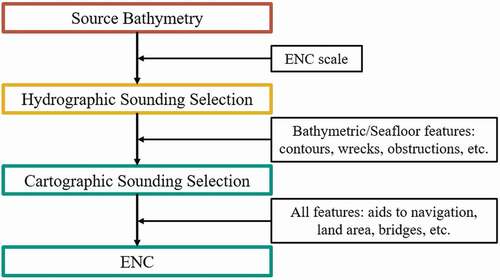
There are also research efforts that attempt to derive a cartographic sounding selection from the source bathymetry (e.g. Haigang et al., 1999; Lovrinčević, 2019; Yu, 2018). However, due to the complexity of the procedure and recognized deficiencies with existing approaches (see, Cavanagh, 2019), cartographic sounding selection remains a semi-manual process (Kastrisios & Calder, 2018). The lack of a fully automated solution results in the continued practice of identifying soundings for chart display from the hydrographic sounding selection. Thus, the focus of this work is to produce an optimal hydrographic sounding selection, from which cartographers can select chart-ready soundings or utilize as input into another algorithm. Consequently, the generalization process must adhere to the aforementioned cartographic constraints as much as possible to avoid carrying errors into the cartographic sounding selection and, ultimately, the final cartographic product. This workflow is summarized in Figure 1.

Figure 1. Workflow from source bathymetry to ENC.

Traditionally, the hydrographic sounding selection was in the form of a sheet of paper, known as a smooth-sheet. The smooth-sheet was a manual shoal-bias selection from the source data, where the physical dimensions of the paper and label sizes limited the quantity of soundings that could be included. Figure 2 shows an example of a smooth-sheet (Putnam, 2013).

Figure 2. Example smooth-sheet (Putnam, 2013).

Today with digital cartographic production systems, hydrographic sounding selections are stored in a digital format, namely point clouds. Existing algorithms in the literature to derive such point clouds are intrinsically limited in that they do not consider the final DCM of the data during generalization and rely on simple distance metrics. Moreover, these approaches require user-defined input parameters, which can significantly affect the results depending on the selected values. This results in hydrographic selections with an enormously large number of soundings that are still difficult to work with for the semi-manual cartographic sounding selection.

In this work we introduce a novel sounding label-based generalization algorithm to provide a shoal-biased hydrographic sounding selection that is product-driven and independent of user-defined parameters. The hydrographic sounding selection produced by the label-based generalization is compared with selections produced by existing radius- and grid-based methods. Furthermore, for the first time in the literature, the hydrographic selections produced by each approach are validated using the four aforementioned cartographic constraints. The incorporated validation aims to serve as a basis for standardizing a performance evaluation method for future automation efforts. It is demonstrated with the support of four test datasets that the proposed label-based generalization algorithm performs the best in regard to the fundamental constraints of nautical cartography: functionality and legibility.

The remainder of this paper is organized in the following manner. Section 2 discusses related work. Section 3 with the accompanying Appendix A (in Supplementary Materials) proposes the new methodology. Section 4 presents experimental results and a comparison to existing algorithms. Finally, Section 5 draws concluding remarks.

2. Related work

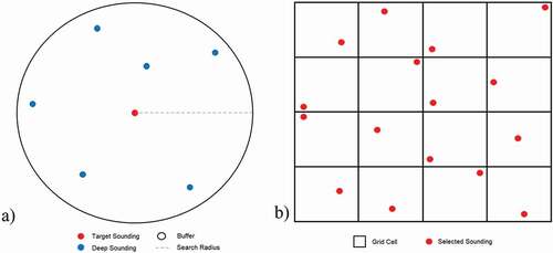
A common approach to hydrographic sounding selection involves using a fixed or variable sized radius (also referred to as a radius of influence) to reduce sounding density (Haigang et al., 2005, 1999; Oraas, 1975). Soundings are sorted from shallow to deep and beginning with the shallowest sounding, the target sounding, a buffer is applied using the input radius value. All of the soundings inside this buffer that are deeper than the target sounding are then removed from the list. The process is repeated for the remaining soundings in the list until all soundings have been examined. Figure 3 illustrates the radius- and grid-based (described later in this section) generalization algorithms, where for the radius-based approach (Figure 3A) the deep soundings are removed in favor of the target sounding.

Figure 3. Common generalization approaches: a) radius-based and b) grid-based.

The main advantage of radius-based approaches is that the output is evenly distributed. Soundings can have equal spacing, in the case of a fixed radius, or exhibit increased spacing with depth, as with a variable length radius that increases with depth. However, these approaches violate both legibility and functionality constraints by under- and over-generalizing in different regions of the bathymetry.

A fixed-length radius approach seems suitable for generalizing a dataset that covers a mostly flat seafloor topography where the bathymetry does not exhibit a wide depth range. If all depths had the same number of digits composing their labels, for example, the user could set the length of the radius to correspond to the width of sounding label. However, the width of the sounding label is not equal to the height, which means that this approach would still result in legibility and safety constraint violations. Furthermore, this limited depth range and equal sounding label width is not common in most hydrographic surveys, or in the full extent of a nautical chart, and does not accurately generalize bathymetry with broader ranges of depth. This is due to the difference in the number of the glyphs (representation of a digit) and their vertical position that make up the sounding label (see Appendix A for details).

It could be assumed that the use of a variable length radius that increases with depth could help reduce the under- and/or over-generalization that can occur with the fixed length radius, where the user could select a starting radius equal to the label size of the shallowest sounding and the ending radius equal to the deepest sounding label. The shallower depths would be generalized with the smaller radius and the deeper depths would be generalized with the larger radius. However, as shown in Section 4, it is clear that this is not the case for the datasets examined. On the contrary, it is demonstrated that this approach still results in functionality and legibility constraint violations similar to that of the fixed-radius. The problem partially arises from depths within the same depth range that have very different label widths and heights. Depths of 9.9, 10, and 10.1 meters (m), for example, would have very similar radius lengths for generalization; however, their respective depth labels have different heights and widths due to the number of digits and presence of decimal values (see, Figure 4). Hence, depths with only a two decimeter difference can have very different label footprints (see, Section 3.1 and Appendix A).

Figure 4. Over- and under- generalization as a result of the radius-based generalization approaches, where the radius length, R, is based on the width or height of the sounding label and D represents a given glyph.

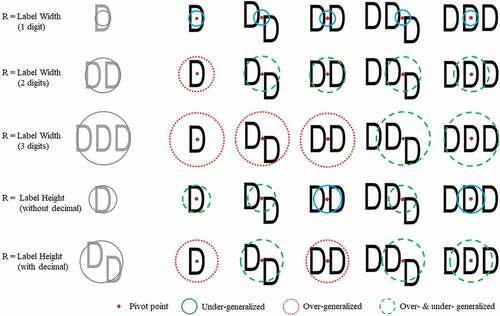
Furthermore, using a circular shape for generalizing bathymetry is not ideal for hydrographic sounding selection, as the sounding label footprint is rectangular (depths without a decimal) or polygonal (depths with a decimal) and the circular shape can over- and/or under-generalize depending on the depth value. Over-generalization occurs when the circle is larger than the label footprint and soundings are removed that could be retained without overlap. Under-generalization occurs when the circle does not cover the entire depth label and soundings are retained that will overlap. Figure 4 shows how over- and under-generalization can occur with the radius-based approaches for labels composing of one, two, or three glyphs (digits), with or without decimals.

Figure 4 also illustrates the increased complexity of label placement in ECDIS portrayal, where the pivot point is not always in the center of the label and can vary depending on the number of digits and the presence of decimals. The pivot point for three-digit labels with no decimal value (far-right labels in Figure 4), for example, is located in the center of the tens column. The pivot point for the two-digit label with a decimal value (second from right labels in Figure 4) is located between the tens and ones columns and also vertically offset.

Another generalization approach involves superimposing a triangular or rectangular grid over the data, and identifying the shallowest sounding for each grid cell (Skopeliti et al., 2020; Tsoulos & Stefanakis, 1997). This concept is illustrated in Figure 3b, where a single sounding has been identified for each grid cell.

A grid-based approach can violate the legibility constraint in many of the same ways as the fixed radius-based approach. The grid cell size is fixed and will under- and over-generalize for bathymetry with broad depth ranges. Furthermore, depending on the grid point of origin as well as grid cell size and shape, soundings can be located in different grid cells, thus resulting in inconsistent outputs based on the implementation. Moreover, as shown in the far-left column of the grid in Figure 3b, soundings can be within close proximity of one another regardless of cell size, which can further add legibility constraint violations. A minimum distance between soundings can be maintained (e.g. Skopeliti et al., 2020), yet, the outcome of both radius- and grid-based approaches remains highly dependent on user-defined input parameters and, as such, they generally result in datasets with considerable functionality and legibility constraint violations. Figure 5 illustrates this further by portraying the vertical profile of a seabed and the resulting sounding selections derived from grid-based (Figure 5a and 5b) and radius-based (Figure 5c and 5d) approaches. The use of different points of origin for the grid-based approach (Figure 5a and 5b), as well as different thinning distances (Figure 5c and 5d) results in different selections. The solid lines for the radius size in Figure 5c and Figure 5d are used to indicate the areas where neighbor soundings have not yet been evaluated, and the dashed lines indicate areas that have been previously evaluated and a shallow sounding was selected.

Figure 5. Vertical profile of seabed and the selection with grid- (a, b) and radius-based (c, d) generalization approaches using different grid point of origin (a – b) and radius size (c – d).

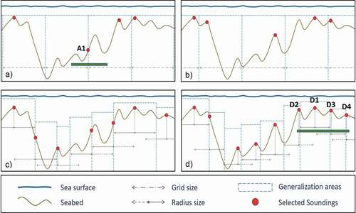
Figure 5a and 5d show soundings that could be potentially selected from either the grid- (A1) or radius-based (D1-D4) approaches. Sounding A1 in Figure 5a is the shallowest depth for the grid cell, but not the shallowest depth within the x-dimension of the A1 depth label (shown by green bar). A peak is present in the grid cell to the right, which would be contained by the depth label of sounding A1. If sounding A1 became a charted depth through the subsequent cartographic sounding selection process, a deeper depth would be displayed in favor of a shallow depth, resulting in a violation of the functionality constraint and danger to navigation. Similarly, for soundings D1-D4 in Figure 5d, the cartographer would have to manually select one of these soundings for chart display in order to avoid label overlap and crowding the chart. Selecting the incorrect sounding would be a violation of the safety constraint. However, our proposed label-based approach would automatically select the correct shallow sounding, D1, and eliminate soundings D2-D4, which are deeper and within the D1 depth label.

In summary, existing algorithms for hydrographic sounding selection are inconsistent and highly dependent on input parameters. Thus, in the following section we propose a label-based generalization algorithm that is product-driven in relation to S-52 and independent of user-defined parameters.

3. Proposed methodology

Our label-based generalization process involves the removal of soundings from the source bathymetry data using label footprints at scale and shoal-bias in order to enforce the aforementioned cartographic constraints to the maximum extent possible. The basis of our approach consists of rounding the depth values to S-52 standards for ENCs, calculating the sounding label footprint, and generalizing the bathymetry using the label footprint while preserving shallow depths. Our approach utilizes bathymetry data represented as a set of points, where the generalization algorithm is agnostic of the data collection method or data distribution.

Section 3.1 with the accompanying Appendix A describes the methods for rounding depth values according to S-52 standards and sounding label dimensions. Section 3.2 describes the algorithm for generalizing the bathymetry using the sounding label footprint.

3.1 Sounding label footprint

Calculating the sounding label footprint requires first rounding the survey depth value and then using sounding label portrayal information and relevant visual perception limits to determine the label footprint at chart scale (see Appendix A). The IHO S-52 publication provides standards for safely rounding depths from surveys to ENCs, where depths ranging from 0 to 31 m are rounded down to the nearest decimeter and depths over 31 m are rounded down to the nearest meter. This rounded depth value is the value displayed on the ENC and is used to calculate the footprint of the sounding label.

The calculation of the label footprint requires the glyph (D in Figure 6) height (D_H), glyph width (D_W), stroke width (S_W), spacing between glyphs (D_S), and label spacing (L_S). A minimum label spacing must be maintained to ensure legibility and avoid confusion between two neighboring labels that can be interpreted as a single label, e.g. a 23 m label from individual labels of 2 m and 3 m. The above values depend on the mapping application, the display medium, expected viewing distance, and human perception limits (e.g. Rytz et al., 1980; HFES, 2007; Ware, 2013; Lakshminarayanan, 2015). The reader is referred to Appendix A for a more detailed analysis of the label footprint. Figure 6 shows a diagram illustrating the variables used to calculate the polygonal footprint, where values are given at millimeters (mm) at scale.

Figure 6. The general case of the polygon label footprint with the label spacing.

Referring to Figure 6, the difference in height is a result of the vertical offset for the decimal value (required by S-52 standards), as described in Appendix A. This example illustrates the complexity of the problem, which cannot be approximated with a single value parameter for use with the radius or grid-based approaches and exemplifies the need for the proposed label-based generalization approach.

3.2 Label-based generalization

Our label-based generalization approach has two components. The first component consists of removing deep soundings directly inside the sounding label footprint to enforce shoal-bias, while the second component removes soundings whose labels overlap with shallower sounding labels.

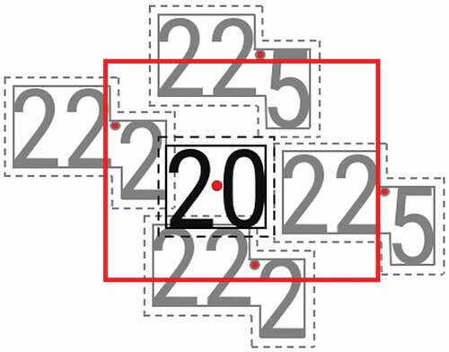
The label-based generalization was initially developed as a single process; however, it was found that the proposed sequential approach resulted in fewer functionality constraint violations. The algorithm for both components is the same, the difference is that the second component uses a larger footprint to generalize the data in order to remove overlapping labels. This is illustrated in Figure 7, where the black rectangle represents the footprint used in the first component and the red rectangle, referred to as the legibility rectangle, is used in the second component of the label-based generalization. In this example, the 22.2 m soundings are within the legibility rectangle and will be eliminated because, when rendered at scale, they overlap with the 20 m target label. Conversely, the 22.5 m soundings are marginally outside the legibility rectangle, and, as such, are retained in the generalized dataset. The example of Figure 7 is one of the many legibility rectangles that have been developed and implemented to account for the various cases of the target and neighboring soundings.

Figure 7. Example generalization footprints for the first (black) and second (red) components of the label-based generalization process.

The input to the first component of the algorithm consists of a set of source soundings and the scale at which the bathymetry data are to be processed. Each input sounding consists of three real values that represent longitude, latitude, and depth, respectively. Such information are maintained in a list, that we call the source soundings list, and the data structures used when processing the input data encode just the indices of the soundings in such list.

The soundings are inserted into a bucketed point-region (PR) quadtree (Samet, 1984), where sounding indices inside the source sounding list are stored in its leaf nodes. A bucketed PR-quadtree recursively decomposes a square domain in the plane containing the soundings by subdividing it into nested square regions, called blocks. Each block has a maximum capacity, specified as input, and it is recursively split into four quadrants when the number of soundings in the block exceeds the capacity. The primary factors influencing the efficiency of the data structure and associated capacity value are related to the data distribution, i.e. uniformity, regularity, and density. Experiments were conducted using the four datasets in this study to test the efficiency of different capacity values and it was found that a capacity value of 0.04% of the number of points achieved suitably efficient results.

An auxiliary list is also created, sorted source soundings, containing the indices of the source soundings sorted from shallow to deep. Beginning with the first element in sorted source soundings, called the target sounding, the label polygon of target sounding is calculated based on the input scale, as discussed in Section 3.1 and Appendix A. This label footprint is then used to traverse the quadtree, where the indices of those soundings that fall inside the label footprint and are deeper than the target sounding are removed from the quadtree. The sounding indices removed during this process are also removed from sorted source soundings, as they no longer require consideration. This process is repeated iteratively on sorted source soundings, until each element of such list has been assessed. The output of this process is the quadtree containing the generalized sounding indices for the first component of the label-based generalization and the generalized soundings in sorted source soundings. Algorithm 1 describes the generalization algorithm in a pseudo-code format.

Table

Algorithm 1: Label-based generalization Input: S, sorted list of source sounding indices Input: L, list of source soundings Input: R, scale of chart Input: Qt, bucketed PR-quadtree of source sounding indices Output: Qt, the bucketed PR-quadtree containing generalized sounding indices

1: for index in S: 2: # Retrieve sounding 3: target_sounding = L[index] 4: # Call function to calculate sounding label footprint 5: label_footprint = get_sounding_label(target_sounding.get_z(), R) 6: # Traverse PR-quadtree and identify indices of soundings inside the label footprint 7: overlap_indices = Qt.traverse(label_footprint) 8: # Remove deep sounding indices from PR-quadtree and source sounding list 9: for overlap_index in overlap_indices: 10: if L[overlap_index].get_z() > target_sounding.get_z(): 11: Qt.remove(overlap_index) 12: S.remove(overlap_index)

The second component of the label-based generalization removes deep soundings whose labels overlap with shallow sounding labels. This is achieved by using Algorithm 1 and a larger legibility footprint calculated based on the label of the target sounding, labels of potential neighbors, and a label separation value (0.75 mm) to maintain legibility among soundings, as described in Section 3.1 and Appendix A.

As previously described, the capacity value for the quadtree is based on a percentage of the total quantity of input soundings. The first component of the label-based generalization process removes a large quantity of soundings, which in turn, significantly reduces the capacity value for the second generalization component. It was found through the testing of the datasets used in this work, that the first generalization component removes approximately 96.7% to 99.2% of the original number of soundings. Thus, the capacity value for the first generalization component would be far too large for the second generalization component and not provide an adequate decomposition of the domain. Therefore, the quadtree is updated using recursive node merging to reflect the change in capacity value.

Overlapping labels are removed by utilizing the updated quadtree and the remaining soundings in sorted source soundings. Beginning with the first element in sorted source soundings, called generalized sounding, the larger footprint of generalized sounding, called the legibility rectangle, is calculated based on the input scale. The legibility rectangle is then used to traverse the PR-quadtree, where the label footprint for each sounding inside legibility rectangle is calculated. Indices of deep soundings whose label overlaps with the label of generalized sounding are removed from the quadtree and sorted source soundings, as they no longer require consideration. This is then repeated for the next element in sorted source soundings, until each element has been assessed. This results in a final set of soundings where sounding labels do not overlap at the selected scale.

4. Experimental results

In this section, we compare the output of the proposed algorithm to the output of the fixed-radius, variable-radius, and grid-based approaches, described in Section 2. Our label-based algorithm has been implemented in Python, and we also developed Python implementations for the other three approaches, because of the lack of availability of existing public-domain implementations.

The hydrographic survey data used in our experiments were identified using the National Centers for Environmental Information (NCEI) bathymetric data viewer portal (National Centers for Environmental Information (NCEI), 2021). The data were selected to be representative of a variety of geographic regions of the U.S., depth ranges of the surveys, and scale of largest ENC in the area. Each of the datasets are horizontally referenced to their respective North American Datum of 1983 Universal Transverse Mercator zone and vertically referenced to mean lower low water. Figure 8 shows the bathymetry for each survey. Table 1 summarizes metadata information for each survey, where the depths are rounded for chart display, as discussed in the previous section.

Table 1. Metadata of the hydrographic surveys used in this work

Dataset	Survey Number	Minimum Depth (m)	Maximum Depth (m)	Average Depth (m)	Largest Scale ENC in the Area
Charleston Harbor, SC	H11861	0.0	19.7	8.9	1:20,000
Narragansett Bay, RI	H11988	0.4	21.9	7.6	1:20,000
Tampa Bay, FL	H12018	1.5	18.2	7.4	1:40,000
Strait of Juan de Fuca, WA	H12626	0.0	138	68	1:25,000

Figure 8. Bathymetry for surveys in a) Charleston Harbor, b) Narragansett Bay, c) Tampa Bay, and d) Strait of Juan de Fuca.

Each dataset was generalized using the proposed label-based algorithm as well as the radius and grid-based approaches. The label polygons for the label-based algorithm were calculated based on those discussed in Section 3.1 and Appendix A. All approaches were processed for largest scale ENC in the region, shown in Table 1.

$B{B}_H=\left[C_H+0.5\times \left(N_D\right)\right]+S_W$

$B{B}_W=C_W\times N_C+C_S\times \left(N_C-1\right)+S_W$

Where (in parenthesis are the values used for ENCs):

BB_H is the bounding box height,

BB_W is the bounding box width,

C_H is the glyph height (2.5 mm),

C_W is the glyph width (1.25 mm),

S_W is the stroke width (0.32 mm),

C_S is the spacing between two glyphs with the stroke width included (1 mm),

N_c is the total number of glyphs of the depth value, and

N_D is the number of decimal glyphs in the depth value ({0, 1}).

Equation 1. Formula for calculating height and width of a symbolized sounding bounding box.

In practice, we are aware of hydrographic offices using a universal value of 0.4 mm at scale (or even as low as 0.1 mm) as the input parameter for radius- and grid-based approaches. However, this value results in an extremely dense set of soundings that is far from being comparable with the label-based approach. Table 2 shows the total soundings from the fixed-radius with a radius length of 0.4 mm, a variable-radius with a minimum length of 0.4 mm and maximum length of 0.8 mm, and grid cell height and width of 0.4 mm to the scale.

Table 2. Total quantity of soundings for each source dataset and the outputs of the radius- and grid-based methods using traditional parameters

Dataset	Source Soundings	Fixed Radius	Variable Radius	Grid-Based
Charleston Harbor, SC	221,494	59,907	41,955	113,569
Narragansett Bay, RI	496,433	120,006	65,455	184,101
Tampa Bay, FL	603,132	55,179	36,827	121,669
Strait of Juan de Fuca, WA	847,461	394,886	190,016	544,048

Due to this, we used input parameters for the radius- and grid-based approaches based on statistics of the depth values for each survey and their corresponding depth label dimensions, shown in Table 1. Using the depth value information in Table 1, we calculate the width and height of the corresponding depth label bounding box for the radius and grid cell dimensions that are given by Equation 1 in mm at scale. These values, described in the following paragraph and summarized in Table 3, further reduce the number of selected soundings and demonstrate our effort to optimize the parameters for the radius- and grid-based approaches. However, as can be seen in Table 4, they still result in denser datasets than the label-based approach. We considered increasing the radii lengths and grid cell sizes to further reduce the number of soundings in the resulting hydrographic selections, however, this would only increase the over-generalization problem described in Section 2 and would not have any solid foundation for comparison with the label-based approach. This further demonstrates the utility of the product-driven label-based approach, which does not require such parameters.

Table 3. Summary of input parameters for radius- and grid-based approaches

Dataset	Minimum Radius Length (mm, m)	Maximum Radius Length (mm, m)	Fixed Radius Length (mm, m)	Grid Cell Height (mm, m)	Grid Cell Width (mm, m)
Charleston Harbor, SC	1.91, 38.2	3.035, 60.7	1.91, 38.2	3.32, 66.4	3.82, 76.4
Narragansett Bay, RI	1.91, 38.2	3.035, 60.7	1.91, 38.2	3.32, 66.4	3.82, 76.4
Tampa Bay, FL	1.91, 76.4	3.035, 121.4	1.91, 76.4	3.32, 132.8	3.82, 152.8
Strait of Juan de Fuca, WA	1.91, 47.75	3.035, 75.875	1.91, 47.75	2.82, 70.5	3.82, 95.5

Table 4. Total quantity of soundings for each source dataset and the outputs of the four generalization approaches

Dataset	Source Soundings	Label-Based	Fixed Radius	Variable Radius	Grid-Based
Charleston Harbor, SC	221,494	1,345	8,681	6,338	4,247
Narragansett Bay, RI	496,433	3,212	16,677	13,017	9,275
Tampa Bay, FL	603,132	830	5,466	3,879	2,337
Strait of Juan de Fuca, WA	847,461	2,946	21,367	13,524	8,465

Fixed radius and grid-based approaches have a single input parameter determining the size of the area for generalization. Thus, the width of the sounding label bounding box at scale for the average depth of each survey was calculated using Equation 1 and halved for the fixed radius approach. Similarly, the variable radius lengths were determined by using the minimum depth as the starting radius length and the maximum depth as the ending radius length. The height and width of the average depth sounding label bounding box were also used for the grid cell size, where the southwest corner of the data set is the point of origin. The only parameter for the proposed label-based algorithm was the target scale, at which each individual sounding label footprint is calculated. Table 3 summarizes the input parameters of the existing approaches for each survey in mm at chart scale and m. This illustrates how sounding labels on a smaller scale chart (Tampa Bay) occupy a larger real-world area compared to larger scales (Narragansett Bay).

The increases between the minimum and maximum radii length in each of the datasets are due to the differences in label widths between the minimum and maximum depths. All of the datasets have a minimum depth label consisting of two digits and a maximum depth label consisting of three digits, where the maximum and average depth label of the Strait of Juan de Fuca data set were the only labels without decimal values.

Ideally, the average value used to calculate the fixed radius length should be between the minimum and maximum radii length. This is not the case for any of the datasets, which is due to the fact that despite the larger value of the average depth, both the average and minimum depths have the same number of digits (two) composing the label. This is important to note, as label widths can change when decimal values are involved and not from just shallow to deep. This further exemplifies the difficulty associated with identifying optimal parameters with respect to the legibility constraint for the radius and grid – based approaches.

Table 4 includes the total quantity of soundings before and after the application of each generalization method for each survey.

All of the generalization approaches resulted in significantly fewer soundings than the original dataset. Our label-based generalization process consistently resulted in the least amount of soundings for each dataset and the grid-based generalization resulted in the second least. The number of soundings for the grid-based approach is directly related to the number of grid cells superimposed over the data. The fixed radius approach resulted in more soundings than the variable radius approach for all of the datasets. This is due to the length of the radii, where the length increases with depth for the variable radius approach, which in turn increases the number of soundings generalized. Conversely, the fixed radius approach uses a consistent radius length, resulting in fewer soundings generalized.

Each of the generalized datasets were subsequently assessed for adherence to the constraints of bathymetric generalization for nautical charts: functionality (safety), legibility, displacement, and shape.

The functionality, or safety, constraint states that depth information on the chart must not appear deeper than the source data. The IHO has an established procedure for validating the shoal-bias nature of a sounding selection, known as the triangle test (International Hydrographic Organization, 2017b). The triangle test states that no sounding in the original bathymetry data should exist within a triangle of charted soundings that is shallower than the least depth of the soundings forming the triangle. Violations of this constraint are assessed by extracting a Delaunay triangulation of the hydrographic selection, and for each triangle, comparing the rounded depth values of the source soundings within the triangle to the rounded depth value of the shallowest sounding forming the triangle. If the shallowest source depth value is less than the shallowest sounding forming the triangle, the source depth and the triangle containing it is marked as a violation.

Violations of the legibility constraint occur when symbolized features over-plot at scale, which makes the chart difficult or impossible to read. The label of each generalized sounding was calculated and used to identify instances where the label intersected that of a neighbor. If the generalized sounding overlapped a neighbor, the legibility constraint violation count was increased by one, resulting in a potential maximum of one violation for each generalized sounding.

The displacement constraint is violated when a sounding is displaced from its original location in the source dataset. Violations of this constraint were identified by assessing if the selected sounding exists in the original source data at the same coordinates.

Finally, the shape constraint aims to ensure that the seafloor morphology is preserved through generalization. The constraint is considered more flexible than others (Ruas & Plazanet, 1997), but it is also the most difficult to evaluate, as different metrics of seafloor characteristics can produce varying results. Moreover, as most relevant to avoid dangers to navigation and maintain chart readability, the other three constraints should take priority over preserving shape. However, seafloor morphology can still be useful for navigation. For example, surface roughness can indicate underwater structures, such as marine habitats, that should be avoided when casting an anchor. In this work, we calculate the surface roughness using the average root-mean square height (Shepard et al., 2001) before and after generalization to assess the change in morphology. Surface roughness is computed by triangulating the soundings using the Delaunay method, and for each vertex, calculating the population standard deviation using the vertex-vertex relationships. The value is reported as the difference before and after generalization, not as a discrete number of violations and should be interpreted as such.

Table 5 summarizes the violations of the cartographic constraints across each dataset and bathymetric generalization approach.

Table 5. Summary of cartographic constraint violations

Dataset	Method	Functionality	Legibility	Displacement	Shape
Charleston Harbor, SC	Fixed Radius	128	8,861	0	0.1764
	Variable Radius	122	6,338	0	0.1895
	Grid-Based	90	4,247	0	0.2505
	Label-Based	68	0	0	0.4587
Narragansett Bay, RI	Fixed Radius	88	16,677	0	0.1179
	Variable Radius	102	13,017	0	0.1305
	Grid-Based	94	9,272	0	0.1610
	Label-Based	80	0	0	0.2885
Tampa Bay, FL	Fixed Radius	68	5,466	0	0.2063
	Variable Radius	68	3,879	0	0.2309
	Grid-Based	53	2,337	0	0.3015
	Label-Based	19	0	0	0.5169
Strait of Juan de Fuca, WA	Fixed Radius	352	21,367	0	0.9546
	Variable Radius	342	13,524	0	1.0659
	Grid-Based	167	8,465	0	1.5198
	Label-Based	150	0	0	2.9008

Our label-based generalization approach resulted in the least violations of the functionality constraint across all of the datasets. Conversely, the fixed radius approach had the most (or tied for most) functionality violations for the Charleston Harbor, Tampa Bay, and Strait of Juan de Fuca datasets. The variable radius approach resulted in the most functionality violations for Narragansett Bay. The grid-based approach had the second least amount of violations for all the datasets, except for Narragansett Bay, where the fixed radius approach had less. Despite significantly more input points than the Charleston Harbor and Narragansett Bay datasets, the Tampa Bay dataset resulted in the least amount of functionality constraint violations across all generalization approaches. The Tampa Bay dataset had the least level of depth value precision (to the mm), which resulted in adjacent soundings with the same depth as the assessed sounding. These adjacent soundings were removed in favor of the assessed sounding, which contributed to the generalization of additional soundings and in turn, less overall output soundings. The Strait of Juan de Fuca had the highest number of input points overall and the highest number of functionality violations across generalization approaches.

Our label-based generalization approach resulted in no violations of the legibility constraint. The fixed and variable radius-based approaches resulted in legibility violations for every generalized point in their respective outputs. The grid-based approach only had three soundings in the Narragansett Bay generalized dataset that did not violate the legibility constraint. The number of legibility violations for these approaches are related to the values used for the radius length and grid cell size. Shorter radii and smaller grid cell sizes can result in under-generalization, which leads to increased legibility violations; however, larger radii and grid cell sizes may lead to over-generalization and increased safety violations (see, Figure 4). Moreover, as sounding labels can increase in size within a specific depth range, e.g. the difference in width between a label value of 21 and 21.5 and the other examples discussed throughout this paper, it is practically impossible to generalize as a function of depth without violating the legibility constraint using the radius- and grid-based approaches. Figure 9 shows the hydrographic selections from the four generalization methods rendered at scale based on the S-52 presentation library, using version 4.3.0 of SevenC’s Analyzer software (SevenCs, 2021).

Figure 9. Sounding label distributions of generalization approaches for the Strait of Juan de Fuca dataset: a) fixed radius; b) variable radius; c) grid-based; and d) label-based.

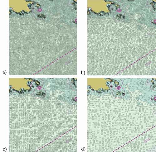
As seen in the output for the label-based approach (Figure 9d), the depth labels are legible and do not overlap, which is not the case for any of the other datasets. Additionally, as described in Section 3, the additional spacing between depth labels for the label-based approach results in soundings that are easily discernable from one another. This increased spacing can result in a slight over-generalization; however, this is in favor of legibility. As such, the increased spacing could be reduced to fit user needs.

None of the approaches resulted in violations of the displacement constraint. This is due to the fact that none of the approaches extract interpolated soundings and the generalized data is derived directly from the source soundings.

Finally, adherence to the shape constraint is directly related to the number of points in the generalized dataset. Across each dataset, the generalization approach that resulted in the largest quantity of soundings had the lowest difference in surface roughness before and after generalization, i.e. surface roughness increased with less selected soundings. The fixed radius approach performed the best in this category, as it resulted in the highest number of soundings, followed by the variable radius and grid-based approaches. Our label-based approach performed the worst, as it consistently had the lowest number of selected soundings. There is a clear trade-off between adhering to the legibility and shape constraints. More selected soundings results in less legibility but an improved representation of morphology and vice-versa. However it should be emphasized that the hydrographic sounding selection from each approach requires further generalization before being used to update an ENC. This will reduce the number of soundings and in turn increase the difference in surface roughness before and after generalization. The greater the number of soundings from the hydrographic sounding selection, the greater the degree of generalization that is required for the final cartographic selection, thus, the greater the effect to the surface roughness. Our approach will require the least generalization, as it results in the fewest number of soundings.

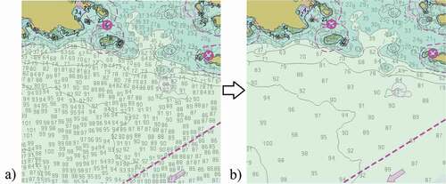
Figure 10 illustrates the need for additional generalization of the hydrographic selection during the cartographic sounding selection for an area of the Strait of Juan de Fuca dataset. Figure 10a shows the hydrographic sounding selection produced from our label-based approach and Figure 10b shows the distribution of the soundings on the current ENC. As explained in this work, the subsequent cartographic selection of Figure 10b is currently a manual process, where the cartographer selects soundings from the hydrographic selection (Figure 10a) based on the particular region and presence of cartographically relevant navigation features, e.g. depth contours, shoreline, rocks, wrecks, etc. It is noted that depth values in Figure 10a and Figure 10ab are different in some regions due to newer bathymetry superseding the survey data used in this work and potential selection issues (as described with the support of Figure 5) from the extremely dense hydrographic selection that was utilized for the production of the chart in Figure 10b.

Figure 10. Sounding label distributions of the a) label-based hydrographic sounding selection and b) cartographic sounding selection present on the current ENC for the Strait of Juan de Fuca dataset.

5. Concluding remarks

This work presented an algorithm for hydrographic sounding selection using the dimensions of sounding labels rendered at scale. The output of the proposed algorithm along with outputs of existing approaches were compared by assessing their adherence to cartographic constraints. Although there exists trade-offs between satisfying all of the cartographic constraints, the proposed label-based algorithm performed the best with respect to the two most fundamental constraints in nautical cartography: safety and legibility. Moreover, the proposed algorithm only requires the scale of the target chart as an input parameter, where the output from radius- and grid-based approaches are highly dependent on input parameters.

We found that the precision of depth measurements can affect the adherence to cartographic constraints for all of the compared approaches. The complication arises from adjacent soundings that have the same depth, where a sounding is retained because it is not technically deeper than the assessed sounding. The datasets used in this work have depths to the millimeter value or less, which helps avoid the issue as depth values with millimeter precision are less likely to be equal. Moreover, the problem was mitigated in this work by removing the neighbor sounding with the same depth; however, this can be a more relevant issue for datasets with less precision.

We also noted that many of the existing approaches in the literature for both hydrographic and cartographic sounding selection lack cartographic constraint-based validations for assessing the quality of the output. As such, the validation approaches presented in this study were used to address this gap. Future work will include building on these validation methods in an effort to better assess the quality of sounding selections derived from different approaches.

The resulting hydrographic selection derived from the proposed algorithm will not contain legibility constraint violations and guarantees that no deeper soundings exist within the label of the portrayed sounding. As such, could be used as input for any manual or automated cartographic sounding selection approach. The cartographic sounding selection further generalizes the hydrographic selection, where the final ENC-ready sounding distribution is based on transportation routes, dangers to navigation, and existing chart features. Utilizing our label-based hydrographic selection as input to the cartographic selection process will result in less cartographic constraint violations, particularly legibility, compared to the other approaches that result in significantly more soundings and constraint violations. Future work will utilize the label-based hydrographic selection as a preliminary generalization method toward a final selection of soundings that complements the other chart features in the representation of the seafloor topography on charts.

Data availability

The data that support the findings of this study are available in figshare at https://doi.org/10.6084/m9.figshare.14474082.v1. These data were derived from the following resources available in the public domain: National Centers for Environmental Information (NCEI) bathymetric data viewer portal (https://maps.ngdc.noaa.gov/viewers/bathymetry)

Disclosure statement

The authors do not report any conflicts of interest.

Supplemental data

Supplemental data for this article can be accessed here.

Additional information

Funding

The work of Christos Kastrisios was supported by the National Oceanic and Atmospheric Administration under grant number NA15NOS4000200. The work of Leila De Floriani was partially supported by the National Science Foundation under grant number NSF IIS-1910766.

References

- Arundel, S. T., & Sinha, G. (2020). Automated location correction and spot height generation for named summits in the coterminous United States. International Journal of Digital Earth, 3(12), 1570–1584. https://doi.org/https://doi.org/10.1080/17538947.2020.1754936
- Cavanagh, G. (2019). Evaluation of current automated BE compilation tools and prospects for improvement. Study Report. Canadian Hydrographic Service.
- Haigang, S., Li, H., Haitao, Z., & Yongli, Z. (2005). A fast algorithm of cartographic sounding selection. Geo-Spatial Information Science, 8(4), 262–268. https://doi.org/https://doi.org/10.1007/BF02838660
- Haigang, S., Penggen, C., Anming, Z., & Jianya, G. (1999). An algorithm for automatic cartographic sounding selection. Geo-spatial Information Science, 2(1), 96–99. https://doi.org/https://doi.org/10.1007/BF02826726
- Human Factors and Ergonomics Society (HFES). (2007). ANSI/HFES 100-2007 Human Factors Engineering of Computer Workstations. Santa Monica, CA, USA.
- International Hydrographic Organization. (2014). IHO transfer standard for digital hydrographic data. Supplementary Information for the Encoding of S-57., Edition 3.1. Monaco, International Hydrographic Bureau. (International Hydrographic Organization Special Publication, S-57).
- International Hydrographic Organization. (2017a). IHO ECDIS Presentation Library. Edition 4.0. (2). Publication S-52. ANNEX A. International Hydrographic Organization Secretariat. Monaco.
- International Hydrographic Organization. (2017b). Regulations of the IHO for International (INT) charts and chart specifications of the IHO, Edition 4.7. International Hydrographic Organization Secretariat. Monaco.
- International Hydrographic Organization. (2021). S-100 geospatial information registry. Portrayal Register. Retrieved 2 March, 2021, from http://registry.iho.int/portrayal/list.do
- Kastrisios, C., & Calder, B. (2018). Algorithmic implementation of the triangle test for the validation of charted soundings. In Proceedings of the 7th International Conference on Cartography and GIS, Sozopol, Bulgaria, June, Bulgarian Cartographic Association. (pp. 18–23). https://doi.org/https://doi.org/10.13140/RG.2.2.12745.39528
- Lakshminarayanan, V. (2015). Visual Acuity. In J. Chen, W. Cranton, M. Fihn (Eds.), Handbook of visual display technology (pp. 1–6). Springer Berlin Heidelberg. https://doi.org/https://doi.org/10.1007/978-3-642-35947-7_6-2
- Lecours, V., Dolan, M. F., Micallef, A., & Lucieer, V. L. (2016). A review of marine geomorphometry, the quantitative study of the seafloor. Hydrology and Earth System Sciences, 20(8), 3207–3244. https://doi.org/https://doi.org/10.5194/hess-20-3207-2016
- Lovrinčević, D. (2019). The development of a new methodology for automated sounding selection on nautical charts. Nase More, 66(2), 70–77. https://doi.org/https://doi.org/10.17818/NM/2019/2.4
- Lu, X., Yan, H., Li, W., Li, X., & Wu, F. (2019). An algorithm based on the weighted network Voronoi Diagram for point cluster simplification. ISPRS International Journal of Geo-Information, 8(3), 105. https://doi.org/https://doi.org/10.3390/ijgi8030105
- MacDonald, G. (1984). Computer-assisted sounding selection techniques. The International Hydrographic Review, 61(1), 93–109. https://journals.lib.unb.ca/index.php/ihr/article/download/23513/27286
- McMaster, R. B., & Shea, K. S. (1992). Generalization in digital cartography. Association of American Geographers.
- National Centers for Environmental Information (NCEI). (2021). Bathymetric data viewer. https://maps.ngdc.noaa.gov/viewers/bathymetry/
- Oraas, S. R. (1975). Automated sounding selection. The International Hydrographic Review, 52(2), 103–115 https://journals.lib.unb.ca/index.php/ihr/article/download/23255/27030
- Putnam, G. R. (2013). Nautical Charts. Project Gutenberg. J. Wiley & Sons. (Original work published 1908).
- Rocca, L., Jenny, B., & Puppo, E. (2017). A continuous scale-space method for the automated placement of spot heights on maps. Computers & Geosciences, 109, 216–227. https://doi.org/https://doi.org/10.1016/j.cageo.2017.09.003
- Ruas, A., & Plazanet, C. (1997). Strategies for automated generalization. In M. J. Kraak, M. Molenaar (Eds.), Advances in GIS research II (Proceedings Seventh International Symposium on Spatial Data Handling (pp. 319–36). Taylor and Francis.
- Rytz, A., Bantel, E., Hoinkes, C., Merkle, G., & Schelling, G. (1980). Cartographic generalization: Topographic maps. Cartographic Publication Series (English translation of publication No. 1). Swiss Society of Cartography.
- Samet, H. (1984). The quadtree and related hierarchical data structures. ACM Computing Surveys (CSUR), 16(2), 187–260. https://doi.org/https://doi.org/10.1145/356924.356930
- SevenCs. (2021). 7Cs Analyzer version 4.3.0. https://www.sevencs.com/
- Shepard, M. K., Campbell, B. A., Bulmer, M. H., Farr, T. G., Gaddis, L. R., & Plaut, J. J. (2001). The roughness of natural terrain: A planetary and remote sensing perspective. Journal of Geophysical Research: Planets, 106(E12), 32777–32795. https://doi.org/https://doi.org/10.1029/2000JE001429
- Skopeliti, A., Stamou, L., Tsoulos, L., & Pe’eri, S. (2020). Generalization of Soundings across Scales: From DTM to Harbour and Approach Nautical Charts. ISPRS International Journal of Geo-Information, 9(11), 11. https://doi.org/https://doi.org/10.3390/ijgi9110693
- Stoter, J., Post, M., van Altena, V., Nijhuis, R., & Bruns, B. (2014). Fully automated generalization of a 1: 50k map from 1: 10k data. Cartography and Geographic Information Science, 41(1), 1–13. https://doi.org/https://doi.org/10.1080/15230406.2013.824637
- Tsoulos, L., & Stefanakis, K. (1997). Sounding selection for nautical charts: An expert system approach. Paper presented at 18th International Cartographic Conference, June 23–27, Stockholm, Sweden: International Cartographic Association.
- University of Utah. (2001). Average character widths. Retrieved April 3, 2021, from https://www.math.utah.edu/~beebe/fonts/afm-widths.html
- Wang, Z., & Müller, J. C. (1998). Line generalization based on analysis of shape characteristics. Cartography and Geographic Information Systems, 25(1), 3–15. https://doi.org/https://doi.org/10.1559/152304098782441750
- Ware, C. (2013). Information Visualization. Elsevier.https://doi.org/https://doi.org/10.1016/B978-0-12-381464-7.00002-8 .
- Weintrit, A. (2018). Clarification, systematization and general classification of electronic chart systems and electronic navigational charts used in marine navigation. Part 2-electronic navigational charts. TransNav: International Journal on Marine Navigation and Safety of Sea Transportation, 12(4). https://doi.org/https://doi.org/10.12716/1001.12.04.17
- Wolfe, E., & Pacheco, P. (2020). Gross benefit estimates from reductions in allisions, collisions and groundings due to Electronic Navigational Charts. Journal of Ocean and Coastal Economics, 7(1), 3. https://doi.org/https://doi.org/10.15351/2373-8456.1121
- Yan, H., & Weibel, R. (2008). An algorithm for point cluster generalization based on the Voronoi diagram. Computers & Geosciences, 34(8), 939–954. https://doi.org/https://doi.org/10.1016/j.cageo.2007.07.008
- Yan, J., Guilbert, E., & Saux, E. (2017). An ontology-driven multi-agent system for nautical chart generalization. Cartography and Geographic Information Science, 44(3), 201–215. https://doi.org/https://doi.org/10.1080/15230406.2015.1129648
- Yu, W., Zhang, Y., Ai, T., & Chen, Z. (2021). An integrated method for DEM simplification with terrain structural features and smooth morphology preserved. International Journal of Geographical Information Science, 35(2), 273–295. https://doi.org/https://doi.org/10.1080/13658816.2020.1772479
- Yu, W. (2018). Automatic sounding generalization in nautical chart considering bathymetry complexity variations. Marine Geodesy, 41(1), 68–85. https://doi.org/https://doi.org/10.1080/01490419.2017.1393476
- Zhang, X., & Guilbert, E. (2011). A multi-agent system approach for feature-driven generalization of isobathymetric line. In A. Ruas (Ed.), Advances in cartography and GIScience. Volume 1: Selection from ICC 2011, Paris (pp. 477–495). Springer Berlin Heidelberg. https://doi.org/https://doi.org/10.1007/978-3-642-19143-5_27
- Zoraster, S., & Bayer, S. (1992). Automated cartographic sounding selection. The International Hydrographic Review, 69(1). https://journals.lib.unb.ca/index.php/ihr/article/view/23255.