Detection of discrepancies between nautical charts and new survey data using GIS techniques

ABSTRACT

Nautical charts are critical for safe navigation as long as they remain updated and trustworthy for the reality they depict. The increase in marine traffic and the growth of available data require that the process of assessing nautical chart adequacy, which consists of comparing information from a new survey with the one published in the ruling cartography, be both fast and effective. In this sense, this work aims to automate the detection of discrepancies between nautical charts and survey data to minimize human effort. We developed a Geographic Information System (GIS) location model based on specific rules derived from three analysis criteria: depth areas, minimum soundings, and bathymetric models. The model produces six outputs, two for each criterion, to support the ultimate human decision. We have tested the model in several hydrographic surveys, such as open waters and harbor surveys, and successfully validated it by comparing results with other available methods, such as current manual processes and Nautical Chart Adequacy Tools (CA Tools). Potential advantages over other methods are also evaluated and discussed, validating the usefulness of this novel approach for the adequacy and completeness evaluation of nautical charts. Our results deliver important benefits by enhancing the GIS techniques for nautical chart production and maintenance.

KEYWORDS:

• Chart maintenance
• electronic navigational chart
• hydrographic survey
• nautical chart
• safety of navigation

1. Introduction

Nautical charts are critical for the safety of navigation (National Oceanic and Atmospheric Administration (NOAA) 2021) (Wolfe & Pacheco, 2020), and they represent, since the fifteenth century, one of the major sources of geographic information (Gaspar & Leitão, 2018). The information depicted in a nautical chart is compiled from several sources (Russom & Halliwell, 1978), using different techniques at different times (Prince, 2017), which are classified in terms of their confidence and quality (International Hydrographic Organization (IHO), 2020; Weintrit, 2018). The need for chart maintenance can derive from multiple factors: 1) natural changes, due to seafloor and water column dynamics; 2) artificial changes, caused by the construction of maritime infrastructures that change depth (dredging) and shoreline configuration; 3) data acquisition changes, as increasingly state-of-the-art surveying methods provide more accurate and detailed bathymetry (Wölfl et al., 2019); 4) and information purpose changes, as the continuous growth of ships’ dimensions (draft) and marine traffic density leads to new routes and navigational restrictions (Haralambides, 2019). These unceasing changes can rapidly turn the nautical charts outdated, diminishing their value and relevance to safe navigation and potentially contributing to maritime casualties (International Hydrographic Organization (IHO), 2018). Therefore, chart maintenance is a never-ending task that should be methodical and objective.

New hydrographic surveys (HS) are often performed, being necessary to assess if the newly acquired data agrees with the information published in the ruling nautical chart. If there exists any discrepancy, it is imperative to evaluate if it has an impact on the safety of navigation and to what degree it does so. Thus, Chart Update Urgency (CUU) can be classified into three categories: 1) urgent, when the discrepancies have a critical impact on safe navigation; 2) less urgent, when the discrepancies have navigational significance, although not critical; and 3) non-urgent, when the discrepancies do not have navigational significance, but they affect the trueness of the cartographic representation of objects (IHO, 2018). This categorization comprises several criteria, mainly based on the magnitude and location of the discrepancies, which are not always easy to implement and may lead to less objective interpretations (Instituto Hidrográfico (IH), 2020).

The chart production process comprises a few complicated transformations – rounding, simplification, and generalization, which still require remarkable human attention and are only partially computer-assisted (Miao, 2014). The compilation of bathymetry (sounding selection and depth contours generalization) for a nautical chart is one of the most complex and time-consuming processes. The charted bathymetry is usually derived from a more detailed data source, often a high-resolution bathymetric model, requiring some degree of generalization (Kastrisios et al., 2019). This procedure frequently implies some compromises between a set of constraints (Dyer et al., 2022) – legibility, functionality (safety of navigation), morphological and topological (Zhang & Guilbert, 2011). Those are often incompatible with each other (Peters et al., 2014), and may produce a couple of consequences. Firstly, reverse engineering cannot be applied to generalization in a straightforward way, which hampers the comparison between high-resolution survey data and scattered information from the chart. Secondly, the methods used for the validation of charted soundings and depth contours (production phase) may also be applied to the evaluation of chart adequacy considering a new survey (maintenance phase).

Chart adequacy assessment (CAA) represents a challenge to many national hydrographic offices (Masetti et al., 2018). In recent years, data acquisition methods have been improved in terms of their scope, range and resolution (Wölfl et al., 2019). Multibeam Echosounders (MBES) (Le Deunf et al., 2020), Synthetic Aperture Sonars (SAS) (Hoggarth & Kenny, 2014), Light Detection and Ranging (LiDAR), unmanned systems (Mandlburger et al., 2020) and remote sensing satellite imagery (Chénier et al., 2019; Omari et al., 2020) produce larger data volumes with better detail. On the other hand, there has been a global effort to map the world ocean floor (International Hydrographic Organization (IHO), 2021; Mayer et al., 2018), increasing these data sources (crowdsourced bathymetry) (International Hydrographic Organization (IHO), 2020), and the need for systematic assessment (Klemm et al., 2015). Hence, the chart maintenance (update) cycle has become shorter and shorter.

CAA incorporates some technical issues. The modern HS, mainly conducted with MBES, has higher resolution and detail than a nautical chart. The comparison of a high-detailed and multi-purpose bathymetric surface with a special purpose chart, specifically designed to meet the requirements of marine navigation (International Hydrographic Organization (IHO), 2019), can be overwhelming. When done manually, this process often implies reducing the HS information density and creating a few intermediate products, not taking full advantage of the original data. Chart production is not a fully automated process. The workflow that transforms survey data into chart information still has some manual and subjective tasks conducted by the cartographers, which makes it difficult to recreate the process and reconstruct the full bathymetric dataset from the sorted chart information for comparison purposes. Charts present information from multiple sources, with different levels of confidence (Category of Zone of Confidence – CATZOC) based on the following criteria: vertical and horizontal uncertainty; seafloor coverage; and survey characteristics (International Hydrographic Organization (IHO), 2020b).

Despite its indisputable importance, the automation of the CAA process has not been greatly developed. Currently, there is only one publicly available application devoted to this problem – Nautical Chart Adequacy Tools (CA Tools), created by the Center for Coastal and Ocean Mapping (CCOM) as part of the HydrOffice project (Masetti et al., 2018). At the Portuguese Hydrographic Institute (IH), as in most of the hydrographic offices, this process is still being done manually by a visual and analytic comparison between chart information and survey-derived products (sounding selections and depth contours), which makes it subjective and dependent on the cartographer’s experience (IH, 2020).

This work aims to automate the detection of discrepancies between nautical charts and new survey data in order to minimize its biased human component. We developed a Geographic Information System (GIS) model that compares survey data and chart information, locating and quantifying the discrepancies for further classification modeling approaches. Results show that CAA can be partially automated, improving its efficiency and diminishing its subjectivity. Our findings deliver important benefits to hydrographic offices responsible for chart production and maintenance.

2. Materials and methods

2.1. Framework

Nautical chart adequacy is a decision problem that can be divided into two sequential procedures: CAA, which identifies discrepancies between survey information and the published nautical chart; and CUU, which assesses if those differences are important, or not, to the safety of navigation and what is the priority for issuing a chart update (IH, 2020). This decision mainly depends on the magnitude and location of the discrepancies (International Hydrographic Organization (IHO), 2018). For instance, due to the expected navigation in an area, in some locations with dense traffic, small discrepancies can be critical, while in other locations, without significant traffic, large discrepancies can be disregarded. These two processes and the hierarchy of the decisions are illustrated in Figure 1.

Figure 1. Hierarchy of the nautical chart adequacy decision, with three alternatives based on three cumulative criteria.

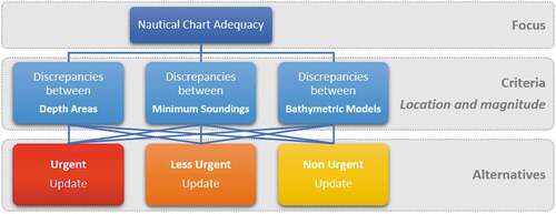
This study focused on CAA, for which we specified three manageable and cumulative criteria that make the results more effective and easier to interpret. The modeling approach is further detailed in section 2.3.

2.2. Data sources and software

2.2.1. Nautical charts

Nautical charts are maps that portray the configuration of the seafloor and the shoreline, showing water depths (soundings) and dangers to navigation (NOAA, 2021). They are created in accordance with the International Hydrographic Organization (IHO), International Maritime Organization (IMO) and International Association of Marine Aids to Navigation and Lighthouse Authorities (IALA) regulations, and they can be made in paper or electronic format (Electronic Navigational Chart – ENC) (Instituto Hidrográfico (IH), 2018). The ENC contains all the critical information for the safety of navigation in a database format with a standardized structure and content (International Hydrographic Organization (IHO), 2000). It can also include supplementary nautical information useful for safe navigation (International Hydrographic Organization (IHO), 2019b).

In this work, we extracted the relevant information from the ENC in vector format and used it as an input in the model. Table 1 describes some of the ENC layers that can be relevant to the analysis. For instance, DEPARE, DEPCNT, DRGARE, OBSTRN, and SOUNDG are important to reconstructing the bathymetric model depicted in the ENC; COALNE, LNDARE, and SLCONS are important to establish frontier conditions; NAVLNE is important to define critical navigation areas. Each of the layers has specific attributes relevant to the analysis. For example, within the ENC DEPARE layer, DRVAL1 (depth range value 1) represents the minimum (shoalest) value, and DRVAL2 represents the maximum (deepest) value of the DEPARE depth range.

Table 1. Relevant Electronic navigational chart (ENC) layers.

Acronym	Object	Geometry
COALNE	Coastline	Line
DEPARE	Depth area	Polygon
DEPCNT	Depth contour	Line
DRGARE	Dredged area	Polygon
LNDARE	Land area	Polygon
NAVLNE	Navigation line	Line
OBSTRN	Obstruction	Point/Polygon
SLCONS	Shoreline Construction	Line
SOUNDG	Sounding	Point

2.2.2. Hydrographic survey

Hydrographic surveys can have different kinds of outputs depending on the technology used in data acquisition and the methodology used in data processing. Usually, the final product consists of one of the following types: 1) point cloud, encompassing all the validated soundings; 2) grid, resulting from a bathymetric gridding method; and 3) sounding selection, based on a suppression radius or another criterion (International Hydrographic Organization (IHO), 2019).

We used grids in raster format with a fixed resolution of 0.5 m and 1.0 m, generated with the Combined Uncertainty and Bathymetric Estimator (CUBE) gridding method (Calder & Wells, 2007). These grids were the survey’s final bathymetric products. Thus, it was possible to exploit as an input in the model the complete validated survey data at the best available resolution.

2.2.3. Software

The model was built using two commercial softwares: CARIS HIPS & SIPS v.11.4 (Teledyne, 2021) and ArcGIS Pro v.2.7 (Environmental Systems Research Institute (ESRI), 2021). CARIS HIPS & SIPS is a hydrographic processing software, and it was used to pre-process the data (i.e. extract ENC layers and survey raster) under an automated processing workflow compatible with ArcGIS Pro and the inputs of the model. ArcGIS Pro was used to execute the spatial analysis and develop the geo-processing model (i.e. ModelBuilder).

2.3. Modeling approach

The GIS model for CAA is divided into four main phases (Figure 2). The model framework is based on the manual process that is being conducted at the IH. The spatial question that the model aims to answer can be defined as: is the nautical chart still adequate now that we have new depth information? Therefore, the model computes the differences between the nautical chart and the new HS information according to international specifications (International Hydrographic Organization (IHO), 2018). Moreover, it locates and highlights those differences. In that sense, it can be described as a location model based on specific predefined rules. The answer to this spatial question is the essence of the CAA process, and it is then used to support the CUU decision.

Figure 2. Framework of the GIS model for assessing chart adequacy.

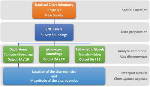
The second step of the framework is related to data preparation. To complete the spatial analysis, we need to select the appropriate layers from each source, ensuring that they contain the required information and that they are interoperable, as well as all the necessary transformations to introduce them as direct inputs into the model. The third phase comprises three cumulative analyses that provide the answers to the spatial question and that are detailed in Sections 2.3.1., 2.3.2., and 2.3.3.

2.3.1. Analysis of depth areas

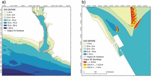
This analysis finds discrepancies between the depth contours of the survey and the corresponding depth areas of the ENC, in the direction of increasing depth (seawards) (IH, 2020). For example, the ENC DEPARE of 5 m to 10 m should not contain the 5 m, or less (e.g. 2 m), depth contour of the survey, as this would mean that in that area there were depths shallower than the ones represented in the ENC, and this could pose a danger to the safety of navigation (Figure 3a).

Figure 3. Example of discrepancies (highlighted by the red lines), a) where the 2 m and 5 m depth contours of the survey are inside the ENC DEPARE of 2 m − 5 m and 5 m − 10 m, respectively. b) the magnitude of these differences is illustrated in a yellow to red classification colour scheme.

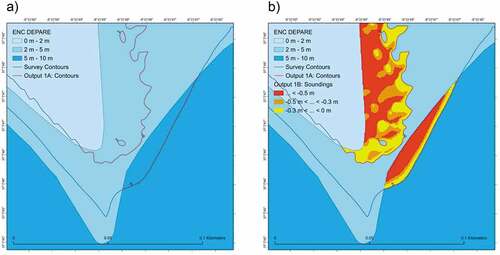
The urgency of the chart update would depend, among other factors, on the Euclidean distance of the discrepancy between corresponding contours, the compilation scale of the ENC and the type of navigation expected in the area (IH, 2020). Occasionally, the Euclidean distance parameter can be misleading because the distance of the discrepancy can be disregarded at some paper chart scale, but the magnitude of the discrepancy can be significant. For this reason, a second output was added, highlighting the magnitude of the differences through warm colors (Figure 3b).

The modeling of this analysis was achieved with an overlay function between the two layers (ENC DEPARE and survey depth contours), selecting the depth contours where depth is ≤ DRVAL1, and with map algebra (Tomlin, 1990), computing the difference between the HS raster and a specific raster built with ENC depth information.

2.3.2. Analysis of minimum soundings

The soundings in the ENC are selected specifically for safety navigation issues and are based on a “shoal biased” pattern (International Hydrographic Organization (IHO), 2018). Generally, they represent the minimum depths in that area. However, IHO recommends that enough numbers of deeper soundings should be retained, in order to assess the full range of depth, for instance, to assist the navigator that uses the echo-sounder to verify its position (International Hydrographic Organization (IHO), 2018). Mariners usually define the navigation plans according to these minimum soundings and the vessel’s characteristics (e.g. vessel draft).

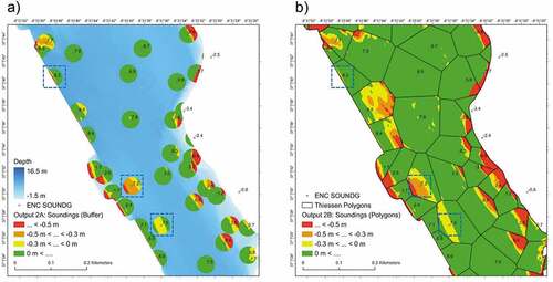
This analysis finds discrepancies between the survey soundings and the minimum soundings represented in the ENC, in a nearby buffer. For example, next to a 17.2 m ENC sounding, there should not exist a 16.9 m survey sounding, as this would mean that the sounding represented in the ENC is not the shoalest in the area, and this could embody a danger to the safety of navigation (Figure 4).

Figure 4. Example of several discrepancies (highlighted by the blue circles) between the survey soundings (in red, with a suppression radius of 50 m) and the ENC SOUNDG (in black).

The urgency of the chart update would depend, among other factors, on the positive or negative sign and magnitude of the discrepancy; the depth ranges in the area (for instance, a discrepancy of 0.5 m has greater significance in a 10 m depth area than in a 50 m depth area); and the type of navigation expected in the area (IH, 2020).

As this analysis involves a buffer definition – the influence area around the ENC SOUNDG, which can make the comparison less objective and user-dependent, we produced two outputs. The first one uses the buffer selected by the user. The second one uses Thiessen polygons (Thiessen, 1911). The modeling for this analysis was achieved with map algebra (Tomlin, 1990), computing the difference between the HS raster and a specific raster built with ENC depth information.

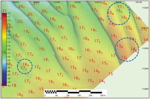
2.3.3. Analysis of bathymetric models

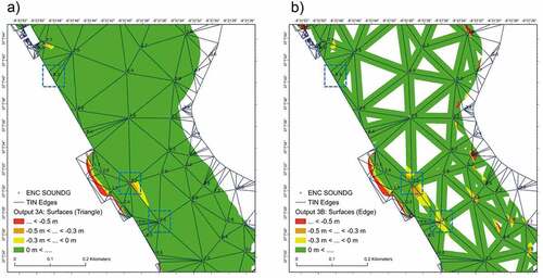
This analysis finds discrepancies between the survey bathymetric model and the triangulated irregular network (TIN) built with the ENC depth information. Contrary to other approaches (Masetti et al., 2018), the tilted triangle test (i.e. if the survey grid has shoaler depths than the ENC TIN), was not considered in this analysis. This test identifies a discrepancy in the area highlighted by the blue polygon (Figure 5(a)), as the survey grid has shoaler depths than the ENC TIN in this zone. It is not entirely clear that this embodies a danger to the safety of navigation, as a mariner cannot realistically expect that the depth variation between two charted soundings is linear, as suggested by the ENC TIN. On the other hand, the mariner can validly conclude that between two charted soundings there is not a shoaler depth than the shoalest of those two, which can be verified by the edge test.

Figure 5. a) Example of the tilted triangle test in a profile view of the seafloor: ENC SOUNDG and the corresponding edge are coloured in black and the survey grid is in red. b) Example of the tri-angle and edge tests: ENC SOUNDG are coloured in black, the triangles are in red and the survey grid is in a blue gradation.

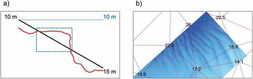
We considered two tests usually followed in the manual process. In the triangle test, none of the survey soundings within a triangle of ENC SOUNDG should be less (shoaler) than the least (shoalest) of the three soundings forming the triangle. In the edge test, none of the survey soundings between two adjacent ENC SOUNDG forming an edge of the triangle should be shoaler than the shoalest of the two soundings forming the edge (International Hydrographic Organization (IHO), 2018). These tests are illustrated in Figure 5(b). Considering the triangle formed by the following soundings: 15.9 m, 17.2 m, and 26 m. Inside this triangle there cannot exist a survey sounding shoaler than 15.9 m (triangle test). Along the edges 15.9 m − 17.2 m, 17.2 m − 26 m and 26 m − 15.9 m, there cannot exist survey soundings shoaler than 15.9 m, 17.2 m and 15.9 m, respectively (edge test). Concerning the edge test, this analysis also involves a buffer definition (edge width), which can make the comparison less objective and user-dependent.

2.4. Model application

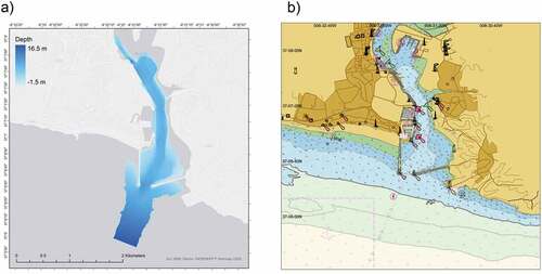
The GIS model was tested in several distinct scenarios, namely, two kinds of HS: open water surveys, without any bounding restrictions; and harbor surveys, with various bounding conditions, such as shoreline infrastructures, breakwaters, and piers. We present the results of a harbor survey, where the analysis can be substantially more complex. This analysis was applied in a HS carried out in 2019, in the harbor of Portimão, a municipality in the district of Faro, in the Algarve region of southern Portugal. The survey was performed with a MBES and the final product was a bathymetric grid with 0.5 m resolution. Depths in the survey range from 16.5 m to −1.5 m (Z axis is positive downwards), and in the ENC from 50 m to −3.8 m (Figure 6).

Figure 6. a) Hydrographic survey extent and depth range. b) ENC of the corresponding area (PT526310).

2.5. Model validation

The GIS model was validated by comparing the results with the other available methods: 1) the manual method (IH, 2020); 2) the straight difference method, defined by the difference between the survey grid and the TIN built with the ENC depth information; and 3) CA Tools (Masetti et al., 2018). The manual method was conducted by an experienced cartographer who coauthored this work. In order to minimize possible biased results, all the manual analysis selected for validation was performed before the development of the GIS model. An analytical flow diagram showing the successive phases of the methodology proposed is shown in Figure 7. On the classification of the efficiency and effectiveness of the different methods, we considered the manual method as the reference (100%) and checked both efficiency (time spent) and effectiveness (completeness of the results and clarity of its interpretation for further decisions). These results are shown in Figure 8.

Figure 7. Analytical flow diagram for the successive phases of the methodology.

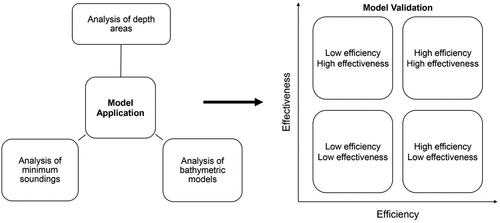
Figure 8. Classification of the different methods efficiency and effectiveness.

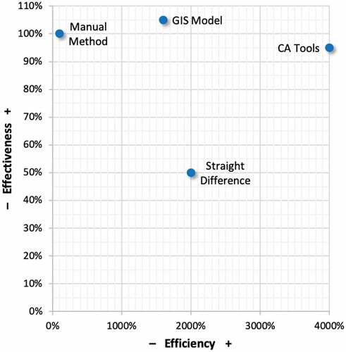
Regarding effectiveness, the comparison with the manual method revealed that the GIS model identified all the situations reported by the cartographer, especially the ones that were later signaled as urgent. In a more subjective inspection, we also considered that it produces results that are easier to interpret as they are presented in a standardized format. The straight difference method identified too many discrepancies and its lack of objectivity decelerates the later priority analysis. CA Tools identified the points that needed review but did not give a clear perspective of what was happening around those points and how the seafloor was evolving compared to the ENC. Therefore, we considered that although its results could support a decision, they were not provided in such a manner that could improve the decision-maker situational understanding (Sanchez, 2009).

Regarding efficiency, although it is a semi-automated process, the GIS model is not the fastest method. As it produces three analyses, it takes more processing time than, for instance, CA Tools. Although having six outputs facilitates the cartographer’s interpretation, it also takes more time to evaluate. When measuring this parameter, we considered both the model processing time and the time spent in preparing the data for ingestion. For instance, in situations where the manual method took 8 hours to complete, the GIS model was 16 times more efficient, taking half an hour. With regard to efficiency, CA Tools performed better than all the other methods, as data preparation was minimal.

3. Results

The results refer to the model application in the HS executed in the harbor of Portimão, in the south of Portugal. The analysis of depth contours identified several locations where the survey depth contours fell outside (seawards) the corresponding ENC DEPARE. Figure 9(a) illustrates the general location of the discrepancies across the HS area, enhancing their Euclidean distances. Figure 9(b) emphasizes the magnitude of the discrepancies in a specific location of the HS area.

Figure 9. Analysis of depth contours. This comparison identifies (in red) the survey depth contours that fall a) outside (seawards) the corresponding ENC DEPARE and b) the magnitude of the depth differences related to those discrepancies.

The analysis of minimum soundings identified some locations where the HS soundings were shallower than the charted depths. An example of these locations is highlighted by the blue squares in Figure 10. Differences above 0 m (colored in green) mean that the survey depths are bigger (deeper) than ENC SOUNDG, thus not representing a danger to safe navigation. The classification scale employed (0 m, - 0.3 m, and - 0.5 m) was considered adequate for special order surveys (International Hydrographic Organization (IHO), 2020c) in harbor areas. As noted, we can identify in both outputs at least three cases (highlighted with blue squares: 8.3 m, 7.2 m, and 7.5 m) where the ENC SOUNDG does not represent the minimum depth in the area, according to the new survey data. The colored classification scale also allows foreseeing discrepancies related to the third analysis: negative differences should be in the direction of lesser (shoaler) soundings or landwards in order to be considered unimportant.

Figure 10. Analysis of minimum soundings. This comparison identifies and classifies the differences between the survey soundings and the ENC SOUNDG, a) within a predefined buffer (25 m, in this example) or b) the corresponding Thiessen polygons.

Comparing the results of the previous analysis with the ones from the analysis of bathymetric models (Figure 11), we notice that this last analysis does not clearly identify the three cases reported before (highlighted by the blue squares). The triangle test (Figure 10(a)) only identified one situation (7.2 m), and the edge test (Figure 11(b)) identified two situations (7.2 m and 7.5 m). This reinforces the principle that the three analyses should be cumulative in order to achieve a complete interpretation.

Figure 11. Analysis of bathymetric models. This comparison identifies and classifies the differences between the survey bathymetric model and a) the ENC TIN: triangle test and b) edge test (buffer of 20 m).

For model validation purposes, we compared the results with other established methods. Figure 11 highlights the different results achieved with other methods for the specific locations previously presented in Figure 9.

In Figure 12(a), CA Tools identifies the 7.2 m sounding as a “possible discrepancy” and signals the 8.3 m sounding as an “untested feature,” probably because it is near the boundary and it may be within a flat triangle. However, it does not identify the 7.5 m sounding, probably because of the parametrization of the threshold difference – it is between 0 and −0.3 m.

Figure 12. Results obtained with a) CA Tools and b) straight difference methods for the same area and with the same input data.

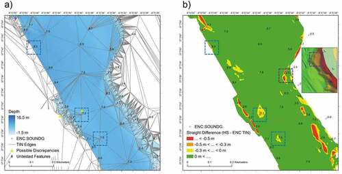
In Figure 12(b), the straight difference method identifies all the discrepancies, but their interpretation and, subsequently, the urgency classification is more complex. For example, this method can give the idea that there is a significant discrepancy near the 2.5 m sounding (highlighted with a magenta square), in the south direction, toward the 6.3 m sounding. Examining the results of the GIS model, we conclude that there is no meaningful discrepancy. This occurred because the depth variation between those soundings (2.5 m and 6.3 m) is not linear. In Figure 11(b), in the shaded relief detail, we can perceive a steep slope and a plateau between those soundings. This illustrates a situation where the tilted triangle test would not be adequate.

4. Discussion

The GIS model was successfully tested with various data pairs (HS versus ENC) with distinct characteristics. Although the results look promising, a broader validation requires more trials. Depending on the study area and on the relevant and available ENC layers, the model might need further adaptations. Nevertheless, this model serves the purposes for which it was developed, in order to support the national hydrographic offices’ workflow. Likewise, this semi-automated model has several advantages over the manual method: 1) it is faster, more effective, and less subjective; 2) it uses the entire survey’s dataset, at the best possible resolution, without the need to downgrade the data and derive intermediate products (sounding selection) to assist the analysis; and 3) it produces results easy to interpret, locating the discrepancies and classifying their magnitude (descriptive statistics).

The model has only two user-configured parameters: the buffer in the comparison between minimum soundings and the buffer in the edge test of the comparison between bathymetric models. As it has been argued that these user values can add some subjectivity, scale, and data density dependent issues (Masetti et al., 2018), we created a second output by computing Thiessen polygons in the analysis of minimum soundings, which may overcome these matters. Concerning the other buffer (edge test), it still remains user-dependent and shall integrate future research work to determine the best buffer size or find geometric alternatives and analogous analysis. Thus, the application of GIS techniques for nautical chart production and maintenance is important for understanding the adequacy and completeness evaluation of nautical charts (Dyer et al., 2022).

Our research presented a good example of a situation where the triangle and edge tests were noticeably not enough to detect significant discrepancies between the survey and the ENC, as defended in other studies (Kastrisios et al., 2019). This demonstrates the importance of the other two additional analyses (depth areas and minimum soundings) and how they complement each other.

Hence, this model stands as a new approach to the CAA problem and an alternative to the other existing automated methods (Masetti et al., 2018). As noted, there is a great difficulty in reconstructing, with full detail, the original bathymetric surface from ENC information. Chart production is not a fully automated process, and the reverse engineering technique can often generate dissimilar reconstructions. This can be partially avoided by building a TIN with linear interpolation between ENC depth information (soundings and depth contours). Yet, some drawbacks may arise. Interpolating ENC sparse information can produce elongated triangles and long edges that reflect the compilation scale of the chart and not the original data density. Assuming linear depth variation between ENC SOUNDG is a rough approach, which does not correctly portray the true seafloor.

We built our GIS model based on three complementing criteria, trying to best replicate the thinking of a mariner when using an ENC, as the three most used layers of bathymetric information are minimum soundings and depth areas defined by depth contours. For instance, these layers are the ones usually used to draw and define navigation plans in restricted waters (Nepomuceno, 2020). The triangle and edge tests (analysis of bathymetric models) are the main principles for validation of charted soundings (International Hydrographic Organization (IHO), 2018). Yet, as demonstrated in previous studies (Kastrisios et al., 2019), and supported by this work, they are not enough for an efficient validation approach. The analysis of minimum soundings identifies if the ENC SOUNDG still remain the shoalest within their radius of influence and how the survey depth is developing in that influence area. For a given suppression radius, ENC SOUNDG should be the shoalest. The analysis of depth areas identifies if the survey depth contours fall inside the corresponding ENC DEPARE. Setting this condition exonerates the need to use the ENC DEPCNT when building the ENC TIN, which often produces elongated triangles, not suitable for the third analysis (analysis of bathymetric models).

In this sense, we did not follow other methods that directly compare the two surfaces (survey grid and ENC TIN) or run the tilted-triangle test (Masetti et al., 2018). As part of the CUU workflow, we considered it more important to identify the critical discrepancies for safe navigation in an easy-to-interpret approach rather than to identify all the discrepancies.

5. Conclusions

Continuous growth of marine traffic and bathymetric data sources demand an effective and efficient CAA process, in order to keep the nautical charts updated and relevant for safe navigation. Thus, the automation of this process and the improvement of its objectiveness can bring important benefits to the hydrographic offices responsible for chart production.

The proposed GIS model achieved good results when compared with other manual and automated methods. Nevertheless, chart production is not a fully automated process, and its overarching goal is to publish information that guarantees the safety of navigation. Therefore, we recommend that this model be employed to assist the cartographer’s analysis and support its decisions, in conjunction with other well-established methods, as it provides purposeful benefits to human action.

Future work will focus on improving the model regarding ENC layers import procedure (for instance, including other relevant layers to the analysis: OBSTRN, NAVLNE, DRGARE), and buffer definition (edge test). Also important would be developing and integrating the CUU workflow, creating additional layers (for example, critical areas for navigation) that, with an overlay analysis and toward a set of criteria, could automatically help to classify CUU. Finally, the application of the model to areas with complex bottom characteristics should also be considered.

Acknowledgements

The authors would like to thank the institutional support provided by the NOVA Information Management School (NOVA IMS), and the Portuguese Hydrographic Institute (IH).

Disclosure statement

No potential conflict of interest was reported by the author(s).

Data availability statement

The data that support the findings of this study are available in figshare at https://doi.org/10.6084/m9.figshare.19217520.v1

Additional information

Funding

This study was partially supported by the FCT (Fundação para a Ciência e a Tecnologia) under the projects PTDC/CTA-AMB/28438/2017 - ASEBIO and UIDB/04152/2020 - Centro de Investigação em Gestão de Informação (MagIC).

References

- Calder, B. R., & Wells, D. E. (2007). CUBE user’s manual. Center for coastal and ocean mapping. UNH Joint Hydrographic Center, University of New Hampshire. https://scholars.unh.edu/ccom/1217/
- Chénier, R., Omari, K., Ahola, R., & Sagram, M. (2019). Charting dynamic areas in the mackenzie river with RADARSAT-2, Simulated RADARSAT constellation mission and optical remote sensing data. Remote Sensing, 11(13), 1523. https://doi.org/10.3390/rs11131523
- Dyer, N., Kastrisios, C., & De Floriani, L. (2022). Label-based generalization of bathymetry data for hydrographic sounding selection. Cartography and Geographic Information Science, 49(4), 338–353. https://doi.org/10.1080/15230406.2021.2014974
- Environmental Systems Research Institute (ESRI). (2021). ArcGIS Pro, version 2.7. https://www.esri.com/products/arcgis-pro
- Gaspar, J. A., & Leitão, H. (2018). What is a nautical chart, really? Uncovering the geometry of early modern nautical charts. Journal of Cultural Heritage, 29, 130–136. https://doi.org/10.1016/j.culher.2017.09.008
- Haralambides, H. E. (2019). Gigantism in container shipping, ports and global logistics: A time-lapse into the future. Maritime Economics & Logistics, 21(1), 1–60. https://doi.org/10.1057/s41278-018-00116-0
- Hoggarth, A., & Kenny, K. (2014). Using synthetic aperture sonar as an effective hydrographic survey tool. Oceans - St. John’s IEEE (pp. 1–12). https://doi.org/10.1109/OCEANS.2014.7003108.
- Instituto Hidrográfico (IH). (2018). Cartografia Náutica em Vigor. https://www.hidrografico.pt/op/41
- Instituto Hidrográfico (IH). (2020). PT.HI.22 – Análise de Dados Topo-Hidrográficos para Avaliação da Necessidade de Atualização Cartográfica. Instituto Hidrográfico.
- International Hydrographic Organization (IHO). (2000). S-57 – IHO transfer standard for digital hydrographic data. International Hydrographic Organization.
- International Hydrographic Organization (IHO). (2018). S-4 – regulations of the IHO for international (INT) charts and chart specifications of the IHO. International Hydrographic Organization.
- International Hydrographic Organization (IHO). (2019). S-102 – bathymetric surface product specification. International Hydrographic Organization.
- International Hydrographic Organization (IHO). (2019b). S-32 – IHO hydrographic dictionary. International Hydrographic Organization. 2019.
- International Hydrographic Organization (IHO). (2020). B-12 – guidance on crowdsourced bathymetry. International Hydrographic Organization.
- International Hydrographic Organization (IHO). (2020b). S-44 – IHO standards for hydrographic surveys. International Hydrographic Organization.
- International Hydrographic Organization (IHO). (2020c). S-67 - mariner’s guide to accuracy of depth information in Electronic navigational charts (ENC). International Hydrographic Organization.
- International Hydrographic Organization (IHO). (2021). C-55 – status of hydrographic surveying and charting worldwide. International Hydrographic Organization.
- Kastrisios, C., Calder, B., Masetti, G., & Holmberg, P. (2019). Towards automated validation of charted soundings: Existing tests and limitations. Geo-Spatial Information Science, 22(4), 290–303. https://doi.org/10.1080/10095020.2019.1618636
- Klemm, A., Pe’Eri, S., Freire, R., Nyberg, J., & Smith, S. M. (2015). Nautical chart adequacy evaluation using publicly-available data. US Hydrographic Conference, Durham. https://scholars.unh.edu/ccom/14
- Le Deunf, J., Debese, N., Schmitt, T., & Billot, R. (2020). A review of data cleaning approaches in a hydrographic framework with a focus on bathymetric multibeam echosounder datasets. Geosciences, 10(7), 254. https://doi.org/10.3390/geosciences10070254
- Mandlburger, G., Pfennigbauer, M., Schwarz, R., Flöry, S., & Nussbaumer, L. (2020). Concept and performance evaluation of a novel UAV-borne topo-bathymetric LiDAR sensor. Remote Sensing, 12(6), 986. https://doi.org/10.3390/rs12060986
- Masetti, G., Faulkes, T., & Kastrisios, C. (2018). Automated identification of discrepancies between nautical charts and survey soundings. ISPRS International Journal of Geo-Information, 7(10), 392. https://doi.org/10.3390/ijgi7100392
- Mayer, L., Jakobsson, M., Allen, G., Dorschel, B., Falconer, R., Ferrini, V., Lamarche, G., Snaith, H., & Weatherall, P. (2018). The Nippon foundation—GEBCO seabed 2030 project: The quest to see the world’s oceans completely mapped by 2030. Geosciences, 8(2), 63. https://doi.org/10.3390/geosciences8020063
- Miao, D. (2014). Gradual Generalization of Nautical Chart Contours with a B-Spline Snake Method [ Doctoral dissertation]. University of New Hampshire.
- Nepomuceno, G. P. (2020). Estudo sobre a utilização do ECDIS na execução danavegação em águas restritas [ MSc Thesis]. Escola Naval, Alfeite.
- Omari, K., Chenier, R., Touzi, R., & Sagram, M. (2020). Investigation of C-band SAR polarimetry for mapping a high-tidal coastal environment in northern Canada. Remote Sensing, 12(12), 1941. https://doi.org/10.3390/rs12121941
- Peters, R., Ledoux, H., & Meijers, M. (2014). A Voronoi-based approach to generating depth-contours for hydrographic charts. Marine Geodesy, 37(2), 145–166. https://doi.org/10.1080/01490419.2014.902882
- Prince, M. (2017). Accuracy and reliability of chart, AA411302. Australian Hydrographic Service. https://www.hydro.gov.au/prodserv/important-info/accuracy_and_reliability_of_charts.pdf
- Russom, D., & Halliwell, H. R. W. (1978). Some basic principles in the compilation of nautical charts. The International Hydrographic Review, 55(2), 11–19. https://journals.lib.unb.ca/index.php/ihr/article/view/23664
- Sanchez, A. (2009). Leveraging Geospatial Intelligence (GEOINT) in mission command. School of advanced military studies. United States army command and general staff college.
- Teledyne. (2021). Caris Hips and Sips, version 11.4. https://www.teledynecaris.com/en/products/hips-and-sips/
- Thiessen, A. H. (1911). Precipitation averages for large areas. Monthly Weather Review, 39(7), 1082–1089. https://doi.org/10.1175/1520-0493(1911)39%3C1082b:PAFLA%3E2.0.CO;2
- Tomlin, C. D. (1990). Geographic information systems and cartographic modeling. Prentice Hall.
- Weintrit, A. (2018). Reliability of navigational charts and confidence in the bathymetric data presented. Zeszyty Naukowe Akademii Morskiej W Szczecinie, 54(126), 84–92. https://doi.org/10.17402/289
- Wolfe, E., & Pacheco, P. (2020). Gross benefit estimates from reductions in allisions, collisions and groundings due to Electronic navigational charts. Journal of Ocean and Coastal Economics, 7(1), 3. https://doi.org/10.15351/2373-8456.1121
- Wölfl, A. C., Snaith, H., Amirebrahimi, S., Devey, C. W., Dorschel, B., Ferrini, V., Huvenne, V. A. I., Jakobsson, M., Jencks, J., Johnston, G., Lamarche, G., Mayer, L., Millar, D., Pedersen, T. H., Picard, K., Reitz, A., Schmitt, T., Visbeck, M., Weatherall, P., & Wigley, R. (2019). Seafloor mapping–the challenge of a truly global ocean bathymetry. Frontiers in Marine Science, 6, 283. https://doi.org/10.3389/fmars.2019.00283
- Zhang, X., & Guilbert, E. (2011). A multi-agent system approach for feature-driven generalization of isobathymetric line. In A. Ruas (Ed.), Advances in cartography and GIScience (pp. 477–495). Springer. https://doi.org/10.1007/978-3-642-19143-5_27