Using remote sensing data to derive built-form indexes to analyze the geography of residential burglary and street thefts

ABSTRACT

By deploying remotely sensed data together with spatial statistical modeling, we use regression modeling to investigate the relationship between the density of the built environment and two types of crime. We show how the Global Human Settlement Layer (GHSL) data set, which is a measure of building density generated from Sentinel 2A satellite imagery, can be used to create different indexes to describe the built environment for the purpose of analyzing crime patterns for indoor crimes (residential burglary) and open space crimes (street theft). Analysis is at neighborhood level for Stockholm, Sweden. Modeling is then extended to incorporate six planning areas which represent different neighborhood types within the city. Modeling is further extended by adding selected social, economic, demographic and land use variables that have been found to be significant in explaining spatial variation in the two crime categories in Stockholm. Significant associations between the GHSL-based indexes and the two crime rates are observed but results indicate that allowance for differences in neighborhood type should be recognized. Average income and transport hubs were also significant variables in the investigated crime categories. The article provides a practical demonstration and assessment of the use of high-resolution satellite data to examine the association between urban density and two common types of crime and offers reflections about the use of satellite image data in crime analysis.

Key policy highlights

• Data Quality and Standardization: Encourage the testing and standardization of methods and measures using remote sensing data, in particular satellite imagery, as a basis for research on urban crime and practical use in urban safety interventions.

• Open Access to Data: Push for policies that promote open access to remote sensing data in research and practice, especially satellite imagery. This is of particular importance in resource-poor urban environments, especially in countries of the Global South where official statistics are not available or are not regularly updated. Open data, such as the one used in this study, provides evidence, fosters innovation, and is the basis for sustainable urban governance.

• Evidence-Based Resource Allocation: Highlight the importance of using remote sensing data and methodologies to inform resource allocation decisions in law enforcement agencies. Advocate for policies that prioritize data-driven strategies to address crime concentrations and allocate resources efficiently.

KEYWORDS:

• Satellite imagery
• GHSL
• burglaries
• street theft
• spatial regression

Introduction

With past and ongoing rapid increases in urban populations, an important focus of discussion in the last decades has been on the need to create livable, safer and sustainable urban environments for all (UN-Habitat, 2018). The UN’s Sustainability Development Goals (UN-SDG, 2015) have provided a framework for interventions needed to improve the quality of life for urban populations. Both the physical and social environments have been investigated for the purposes of improving safety and for crime prevention (Dempsey et al., 2011; Zahnow et al., 2021).

Spatial analytical methods have proved to be invaluable in the field of criminology, providing insights into the spatial patterns and dynamics of crime (Kounadi et al., 2020). By examining the geographical distribution of criminal incidents, hotspot analysis can identify high-crime areas and guide targeted law enforcement efforts. It has long been recognized that geographical variation in the distribution of crime events and criminality in large urban areas is correlated with the social, economic and demographic characteristics of neighborhoods (for an extensive review see for example Bottoms (2012)). However, other characteristics of urban areas also correlate with small area crime statistics including features of the built environment such as housing type and density (Bottoms & Wiles, 1988), street configuration and density (Weisburd et al., 2012), street lighting and the distribution of certain services such as bars selling alcohol and transit stops (He & Li, 2022). The distribution of the natural environment within cities such as green areas and parks (Groff & McCord, 2012), is also often relevant for the study of crimes such as rape or vandalism that take place in urban public spaces.

Official police statistics have been used to analyze crime distributions and to assist with the implementation of crime prevention strategies (Bernasco & Elffers, 2010). Although official police data still provide the most reliable indicators of crime and victimization, such data are not always easily accessible. Other issues with police data have to do with the way the police operate which can affect their recorded crimes. For example, a policy of targeting car crime could see a spike in recorded car crimes. Duplicate crimes, wrong addresses or dates, missing records are just some of the issues that have to be faced when working with police recorded crime data.

This study focuses on assessing the relationship between characteristics of a city’s built environment and crime events using remote sensing data. Historically, data on urban environments, both built and natural, have been obtained through fieldwork but this approach may be time consuming and costly and, in some instances, impractical. An alternative may be to use preexisting conventional (land use) data but that may not be in a form convenient for comparing against crime data using statistical methods. For example, they may be held in paper map form with unknown levels of accuracy. In resource poor urban environments especially in countries of the Global South – a term broadly used by the World Bank to refer to countries characterized by low income, dense population, poor infrastructure, and often political or cultural marginalization in Asia, Africa, Latin America, and Oceania (Arbab, 2019). Conventional data may interrogate with assess: available, making it difficult to assess the detailed spatial dynamics of crime. Meanwhile, fine-grained remote sensing images are free and available worldwide (such as those from the Copernicus Sentinel-2 mission with 10m resolution) making them a potential source of information about the characteristics of the built and natural environments of a city.

This article reports results obtained from using remotely sensed imagery to capture city-wide information about a city’s environments at fine geographical scales. Using remote sensing methods digital data can be assembled about land cover, structure and texture relating to the built environment, the amount of vegetation present, height of buildings and measures of illumination for example. More detailed information may also be obtained on such features as pavements, rooftops and fences which also can be helpful predictors in the study of urban criminogenic environments (Sohn, 2016). Although recent research has explored the potential of google street views and other fine grained remote sensing data to capture information about the urban environment (Hipp et al., 2022; Khorshidi et al., 2021) this study does take a different approach using instead widely available satellite images, such as Sentinel-2A imagery.

The Global Human Settlement Layer (GHSL) dataset, as described in the Global Human Settlement – GHSL Data and tools overview provided by the European Commission (European Commission [EC], 2023), is a freely available resource that quantifies the characteristics of urban environments. This dataset is a globally available map representing the building density. It was generated using advanced technology, specifically a Convolutional Neural Network (CNN) for image classification, as outlined in Corbane et al. (2021), which processed imagery from the Sentinel-2A satellite mission operated by the European Space Agency (ESA). Sentinel-2A imagery was chosen due to its widespread availability as open data and its high spatial and spectral resolutions. The GSHL is stored as a raster layer with a pixel size of 10m × 10m. The pixel values represent the density of the building within each cell, ranging from 0 (no buildings) to 100 (completely built).

In this study, the GHSL dataset serves as a critical component in assessing the relationship between urban features represented by the GHSL building density index and crime data at the city level. Recognizing that the criminogenic significance of urban environments can vary across different types of neighborhoods, the statistical analysis incorporates an interaction between the GHSL index and a classification system that categorizes Stockholm into six distinct neighborhood types. This approach, as inspired by Corbane et al. (2021), enables a more nuanced evaluation of how urban characteristics impact crime rates in various contexts. Furthermore, the analysis takes into account additional factors that are traditionally associated with crime patterns in Stockholm. These factors include conventional land use and various social and economic variables, which are sourced from existing literature on crime in Stockholm. By controlling for these variables, the study aims to provide a comprehensive understanding of the complex relationship between urban environments, neighborhood types, and crime in Stockholm. This article is structured in the following way. Section 2 includes a review of key inputs from urban crime research into the links between the built and natural environment and crime in urban areas followed by a short review of the use made to date of remote sensing data in criminology. Section 3 describes the study area, the data used and the methodology. Section 4, presents results which are discussed in section 5. In section 6 we reflect on the work reported and suggest directions for future work.

Context and theoretical background

Crime links to particular built and natural urban environments

The association between high-density land use (e.g. dense concentrations of buildings, especially houses, and streets) and rates of crime have been, and continue to be, the subject of research. Such an association, where it exists, may be direct and positive with high-density land use providing a spatial concentration of opportunities and suitable cover for would be offenders. The association may be direct and negative with high-density land use having the effect of reducing crime by leading to more supervision of street activities (Twinam, 2014). On the other hand, the association might be indirect with high density associated with social pathologies, such as social disorganization or loss of social cohesion, so that whether high density is correlated with a high crime rate may be dependent on the neighborhood type and the socio-economic composition of the resident and/or transient populations (Stucky & Ottensmann, 2009). Social Disorganization Theory investigates the relationship between the social structure and characteristics of neighborhoods or communities and the occurrence of crime and deviant behavior in those areas (Shaw & McKay, 1976).

Elements of the built environment are associated with high crime rates in particular places (MacDonald, 2015). Criminological research shows that certain urban environments attract disproportionally large amounts of crime having the capacity to draw-in and/or generate crime (Brantingham & Brantingham, 1995) or to be crime radiators and/or crime absorbers (Bowers, 2014). This work links to the “law of crime concentration at places” (Weisburd, 2015), the phenomenon that many crimes are concentrated in very specific small areas of a city. The combination of particular physical environments with the daily rhythmic patterns and “routine activities” of individuals (Cohen & Felson, 1979; Eck & Weisburd, 1995), together with the “awareness space” of offenders (Brantingham, 1984) underpin attempts to explain this phenomenon. Measures of vegetation, street segments, and characteristics of the built environment such as building height and housing type are characteristics of the physical environment that have all been linked to the occurrence of crime events. For example, street width has been associated with burglaries (White, 1990), vegetation presence has been linked to crime patterns, both negatively and positively (Kuo & Sullivan, 2001; Michael & Hull, 1994), as has building height (Newman & Franck, 1982).

Since the 1970s, principles of Crime Prevention Through Environmental Design (CPTED) (Jeffery, 1972), a situational approach to crime prevention, have incorporated the importance of built and natural environments in crime prevention in two ways: the “natural surveillance” (Jacobs, 1961) and the “defensible space” (Newman, 1972) models. The emphasis shifts from concerns about urban density toward a focus on urban design. Jacobs argued the importance of developing land use structures that would encourage population mixing and interaction throughout the day the effect of which was to promote natural surveillance. Natural surveillance means designing urban areas for maximum visibility (balconies, large shop windows, avoiding the creation of poorly lit areas and dead-ends) and promoting land uses that foster population interaction (such as play areas associated with high rise apartment blocks). The “defensible space” model by contrast seeks to develop urban spaces in ways that exclude would-be offenders, making it more difficult for them to offend (Newman, 1972). Perhaps the ultimate expression of this is the gated community, but wherever structures are put in place that make it more difficult for the would-be offender to gain access (e.g. locked gates on alleyways behind terraced housing; target hardening using code locks on doors to high rise apartments) can be said to be applying the ideas behind defensible space (Clarke, 1983). The same is true of situational crime prevention measures undertaken by police forces to reduce crime rates in specific areas (Clarke, 1983; Newman, 1972). Such defensible spaces might be specific buildings, blocks or neighborhoods. When compared with one another, these environments share a number of commonalities in terms of their physical environment but also levels of maintenance that affect crime opportunities.

We conclude that research findings to date highlight the nuanced, indeed contested, nature of the association between urban density and crime and point to the continuing need to explore the question using appropriate data and methodologies.

Spatial analysis in criminology

Spatial analytical techniques have revolutionized the field of criminology by providing a powerful framework for understanding the spatial patterns and dynamics of criminal activities. Crime incident reports, offender profiles, census data, environmental data and remote sensing data can be integrated within a GIS framework to develop comprehensive spatial models. By leveraging spatial data (Li et al., 2023), statistical analysis (Horsefield et al., 2023), and mapping visualization, researchers can gain valuable insights into the spatial distribution of crime incidents, the identification of crime hotspots, and the exploration of underlying socio-economic and environmental factors associated with criminal behavior.

Through the application of hotspot analysis, spatial analysis techniques help identify high-crime areas that require targeted intervention and resource allocation (Leśniak et al., 2022). Law enforcement agencies and policymakers can utilize this information to strategically deploy resources and implement crime prevention strategies in these hotspots. The use of spatial analysis in this context enables a proactive and targeted approach to crime prevention, maximizing the impact of limited resources and efforts.

Spatial regression models have become essential tools for examining the relationship between crime and various socio-economic and environmental factors (Song et al., 2017). By integrating spatial data with statistical techniques, researchers can assess the influence of factors such as poverty rates, educational attainment, population density, or proximity to specific facilities on crime patterns (Demotto & Davies, 2006). This multidimensional analysis helps uncover the underlying mechanisms driving criminal activity and provides valuable insights for policymakers and practitioners in designing effective interventions.

Using remote sensing data to study crime patterns

There is a small but steadily growing literature using remotely sensed data to study the effects of the physical environment on various types of acquisitive crime (Ceccato, V. & Ioannidis, I., 2024). Research has provided evidence that data obtained from remote sensing imagery can capture particular situational characteristics of the natural, built and social environments that are relevant to crime occurrence. Studies have shown, for example, associations between crime events and: illumination levels (Liu et al., 2020; Zhou et al., 2019); urban change (Algahtany & Kumar, 2016; Mansor et al., 2019); density of vegetation and tree coverage (Chen et al., 2016; Wolfe & Mennis, 2012); characteristics of the urban fabric such as building density, roof types, presence of water and shadows (López-Caloca et al., 2009; Patino et al., 2014); presence of slum areas (Duque et al., 2015).

Patino et al. (2014), used a principal component analysis (PCA) to detect features of the urban environment instead of using a traditional measure of vegetation cover such as NDVI. Homicides were linked to the absence of specific features of the urban environment such as open green spaces, wide roads and large industrial or commercial buildings measured from satellite images. The urban fabric that was more crowded and cluttered have been positively associated with higher homicide rates (Patino et al., 2014). Built up area density and vegetation measurements have been linked to property crimes (López-Caloca et al., 2009). Higher vegetation cover has been linked to lower rates of assault, robbery, and burglary, but not theft (Wolfe & Mennis, 2012). Urban development and change, have shown a positive correlation with criminal activities, particularly violent crime, property crime and cases of drug abuse (Algahtany & Kumar, 2016; Mansor et al., 2019). There is a small but steadily growing literature using remotely sensed data to study the effects of the physical environment on various types of acquisitive crime. Although not many, we found studies that remote sensing data can help in explaining the effect of the physical environment, either positively or negatively, on property and theft crimes.

Crime geography in Stockholm: previous research on burglaries and street thefts

Traditionally, research into the geography of acquisitive crimes including burglary and street thefts have focused on social, economic and demographic characteristics of places as exemplified in the work of Wikström (1991) and Ceccato et al. (2001) for Stockholm. Higher residential burglary rates are associated with areas with higher income levels (area attractiveness) while Ceccato et al. (2001) found an association with higher levels of population turnover (area opportunity). Burglary rates did not vary consistently with distance to the city center, but did reflect the distribution of areas of single-family housing units. Hoppe and Gerell (2019) found that in the case of residential burglaries, near-repeat victimizations peaked within the first week. Other studies in Stockholm found that high-priced properties attracted more residential burglaries. The price of properties was positively associated with surrounding land use functions, such as proximity to water and transport stations (Ceccato & Wilhelmsson, 2011) but negatively associated with the presence of open drug markets and shootings (Wilhelmsson et al., 2021). For thefts of and from cars, Wikström (1991) and Ceccato et al. (2001) found that although most crimes were concentrated in inner city areas due to the presence of commercial, administrative and cultural functions, more affluent areas were also at increased risk. This concentration close to single family houses was explained by higher levels of income, and lower guardianship compared to multi-family houses.

Case study

Study area

Stockholm is the capital of Sweden, the largest city in Sweden and one of the important political, economic and cultural centers in Scandinavia (Nordic_Co-Operation, 2022) with a population of around 975 500 in 2020 (2.4 million in the metropolitan area). The municipality is also divided into 16 planning areas which represents the city’s different building styles. For this study, we have merged categories that show similar characteristics of built environment into six categories as shown in Figure 1.

Figure 1. The study area and the six planning areas.

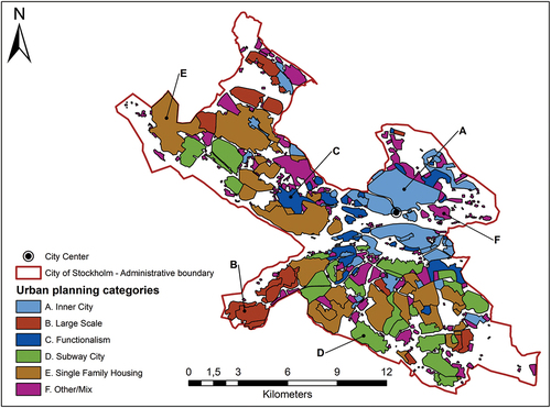
In Appendix A we explain the characteristics of those planning areas. White areas on the map represent areas dominated by the natural environment (water bodies, parks, forests etc.). The black circular point indicates the city hall of Stockholm municipality in the city center. Pictures of these areas are available online (see supplementary material: Planning areas in Stockholm municipality).

Data

Three types of data are used in this study: Police crime records, built environment data obtained from satellite images and land use, demographic and socio-economic data. For a description of the datasets used in this study see Appendix B. The study area as a digital map is divided into 419 basområden (population Max = 9,766, Min = 0, Standard Deviation = 2,107.5) which is one of the smallest statistical units of analysis for which demographic and socio-economic data are available.

By executing a Google Earth Engine script, we extracted the Global Human Settlement Layer (GHS-BUILT-S2) for Stockholm. The GHS-BUILT-S2 dataset represents global built-up areas and expresses their presence as probabilities, all at a high spatial resolution of 10m. This dataset was derived from a cloud free composite of Sentinel-2 satellite images using a Convolutional Neural Networks (CNN) model specifically design to map urban areas (see the implementation detailed in the work of Corbane et al. (2021). It is important to note that the utilization of CNN-based model in the creation of the GHS-BUILT-S2 dataset stands as a significant advance compared to more traditional bands’ ratio indexes such as NDVI (Normalized Difference Vegetation Index) or NDBI (Normalized Difference Built-Up Index). The heightened accuracy of GHSL, when compared to more conventional spectral indices like NDVI or NDBI, can be attributed to several factors. Firstly, the CNN-based model in GHSL transcends the limitations of simple band ratio indexes by simultaneously considering both spatial and spectral features within remote sensing images. This enables the model to discern complex patterns and relationships within urban landscapes, providing a more nuanced and accurate estimation of building density. The GHSL model demonstrates remarkable discriminatory capabilities, effectively distinguishing between buildings and other land cover types, such as bare soil and rocks, even when they share similar spectral signatures. Moreover, GHSL’s CNN model excels in feature extraction, automatically identifying and distinguishing relevant features from the imagery. This capability is particularly beneficial in urban environments where buildings and vegetation often coexist intricately. The model’s ability to intelligently recognize building structures even in areas with substantial vegetation cover contributes significantly to its enhanced accuracy. The robustness of GHSL has been systematically assessed worldwide, with validation against diverse datasets confirming its reliability. This global evaluation ensures the applicability and accuracy of GHSL across a wide range of urban contexts and geographical locations (See et al., 2022). The distribution of the GHSL index in the neighborhood division is available online (see supplementary material: GHSL value per neighborhood).

This model leap results in significantly improved accuracy, as demonstrated through rigorous validation against an independent reference dataset containing building footprints from 277 locations worldwide. This validation process unequivocally confirms the remarkable accuracy of the GHS-BUILT-S2 dataset, which achieves an impressive overall accuracy rate of 80% (Corbane et al., 2021).

The study period covers 2019 and 2020 during which time Stockholm city had approximately 503,000 reported crimes. Two types of crimes were chosen: residential burglary (an example of an “indoor” or “private space” offense) and street theft (an example of an “outdoor” or “public space” offense). These offenses provide also an opportunity to examine the usefulness of the GHSL index in different contexts, using different manipulations of the index. Public space is any usable space accessible to the general public. There were 26,088 reported and mapped street thefts and 8,687 reported and mapped residential burglaries during this two year period. In order to acquire detailed crime data we had to come to an agreement with the Police Authority responsible for the Stockholm region. Those data were in excel format and included data such as the location of the crime (x, y coordinates), timestamp and crime code.

Social, economic and demographic data for 2019 and 2020 were extracted from the Statistical Authority of Sweden (SCB) in excel format. Each entry has a unique code that identifies its spatial reporting unit or neighborhood polygon (basområden). SCB also provides a shapefile with the code of each polygon so that each datum value can be linked to its appropriate polygon. This connection is done with the join function in ArcGIS Desktop. Our social, economic and demographic data are now in a format that we can work with in ArcGIS in order to prepare them for the later step of regression modeling. Data on the variables gender, age, income, employment, nationality and type of house (multifamily apartments and individual units) were downloaded as previous research has shown these variables correlate with the two crime categories in our study.

Land use data, a vector shapefile with cadastral information, was retrieved from the open data website Läntmateriet. It contains all buildings in Stockholm city in polygon shapefile format. The Open data portal for geographical data is available from the municipality of Stockholm. We also retrieved the number of apartments for each of the buildings recorded in the building file. The distance to the city center was defined as the distance to Stockholm’s city hall which also defines the center of the city’s business district. For water bodies we used again Sentinel 2A products. A new index has been introduced recently that can be derived from those satellite images that is called SWI (Sentinel-2 Water Index). Transport nodes were retrieved from the Trafikverket open geodata portal. For instance, the locations of all the main transport nodes such as train stations (pendeltåg), underground stations (tunnelbana) and bus stations (buss) were also added to the dataset.

Data preparation

Because we are investigating residential burglary that is linked to a property and street thefts that happen in public places, we had two different strategies for calculating the pixel by pixel GHSL index for the purposes of modeling the two types of crime. In the case of residential burglary, we captured a GHSL score around all residential buildings. The footprint associated with each residential building was obtained from the Open geodata land use file and then overlaid on the satellite image. Next, a convex hull function was applied to each building together with an additional 50 m radius to capture the surrounding area. The 50 m radius was used since, according to Gehl (2010), 50 meters is the field of view of a person, the maximum distance at which a person can recognize others and also clearly hear shouts for help.

Figure 2 a) shows the cadastral information on the left identifying a building as a white polygon. On the right that buildings convex hull plus the 50 m radius is shown together with the pixelated GHSL scores obtained from the satellite image. The black shading represents pixels with zero built-up GHSL scores (just vegetation), white shading represents pixels which are fully built up. In between, gray shades, represent mixed built-up and vegetation pixels. In the case of street crimes instead of using building footprints on which to base GHSL scores, a 100 m by 100 m fishnet of points was created across Stockholm using ArcGIS after deleting building footprints and water bodies from the area. The area remaining after these deletions is deemed open public space (Fermino et al., 2013) accessible to everyone (although this may not always be the case). The left hand image in Figure 2b) shows an example of a fishnet point whilst the right hand image shows the 50 m radius around that fishnet point (for the same reasons given above) with the same pixel shading as used in Figure 2 a).

Figure 2. a) Cadastral polygons and buffer zones of residential building; b) fishnet point and buffer zone of OSA fishnet.

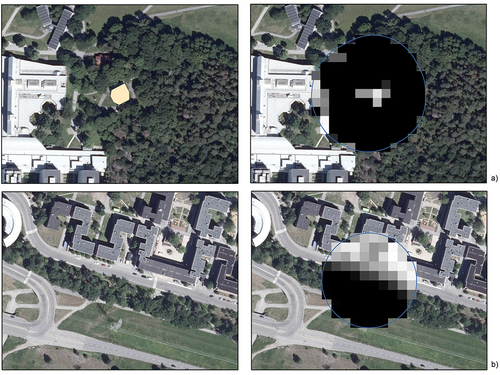
In the case of residential burglaries, a GHSL score is obtained for each building whilst in the case of street thefts, a GHSL score is obtained for each fishnet point. The score for a building or fishnet point is the average value of all the pixels lying within the buffer zone. A pixel is included in a buffer zone if its center point lies within the buffer zone. In the case of a building where there are multiple households (e.g. an apartment block) the GHSL value for that building was multiplied (weighted) by the number of households in the building. For each basomåden, these GHSL values were summed over all buildings in the basomåden. An average value for the basomåden was obtained by dividing this sum by the number of households in the basomåden (here denoted GHSL_B). In the case of fishnet points an average value for a basomåden is obtained by computing the average GHSL value of all the fishnet points lying within the basomåden (here denoted GHSL_O).

Selected social, economic and demographic and land use variables were obtained for each basområden. Total population was used to calculate the percentage of young males aged 15–24 in the population, the percentage of the population above 60 years and the percentage of population born abroad. For the percentage unemployed, the total workforce was used as the denominator. Income was already available from Statistics Sweden, which is a yearly average value per basomåden. This variable was scaled by dividing by 10,000. Population turnover, was calculated by subtracting the population of one year from the population of the previous year, using the total population counts of 2018, 2019 and 2020. They were then averaged to create a single variable for both 2019 and 2020 population turnover since we are investigating crimes together for this 2 year interval. Land use variables were created from different types of land use information. With the spatial join tool in ArcGIS toolbox, the number of land use points for each specific land use type (transport nodes,) in each basomåden was obtained. The count for each land use type was divided by the total area in square kilometers of each basomåden to provide a measure of the density of each land use type. Finally, the six planning areas were converted into 5 dummy variables using the city center planning area as the reference category. All calculations were done in ArcGIS with the field calculator tool. See Appendix B for a detailed description of the dataset.

A crime rate was calculated for the two types of crimes for each basområden. In the case of residential burglary we divide the total number of household burglaries in that basområden by the total number of households and then multiplied by 100 to have a rate per 100 households, which for an apartment block means counting up the number of single family apartments within that block. Ground floor apartments tend to be at greater risk of burglary than upper story apartments but in the absence of any detailed information on how that risk varies no adjustment was made. In the case of street theft, the total number of street thefts in a basområden was divided by the total open space area (Km²) for that basområden and for computational reasons, and to better reflect rates for such small spatial units, this rate was divided by 10.0.

Data modelling

We use spatial regression modeling to examine the relationships between each of the two crime types and the four classes of independent variables: the GHSL indexes (GHSL_B or GHSL_O), the six planning areas, the land use variables and the set of social, economic and demographic variables. A Pearson’s bivariate correlation matrix was first created to examine the strength of the linear relationships amongst the land use variables and amongst the social, economic and demographic variables. Some of these variables were excluded because of the high correlation (R ≥ .6) to avoid multicollinearity between the independent variables. The modeling strategy was to fit a sequence of three models to the data for each of the two offenses as shown below:

• Model 1 contains only the relevant GHSL index as an independent variable.

• Model 2 allows the effect of the GHSL index to vary across the six planning areas. We do this by specifying 5 dummy variables using the inner city planning area (A) as the reference category.

• Model 3 adds to Model 2, a land use variable (density of transport nodes in the basområden) and social/economic/demographic variables (proportion of young males, proportion of population over 60, proportion unemployed, population turnover and average income (x 10-4) in the basområden).

Due to the ordered nature of our modeling strategy, which involves fitting three models of increasing complexity, we took a “theory driven” as opposed to a “data driven” approach to statistical modeling (see for example Waller (2014) and Haining and Li (2020, pp. 27–30)). This means specifying a statistical model that is consistent with our understanding of the modeling problem rather than simply allowing the data to lead the modeling. In following this path, it is still important that the assumptions of regression modeling are satisfied. Whilst there are many assumptions underpinning a valid application of the regression model, a particularly important assumption to check, because of the spatial nature of the data and the danger of model under-specification (omitted variables especially in models 1 and 2), is for residual spatial autocorrelation (Haining & Li, 2020, pp. 4–8). If omitted variables happen to be spatially autocorrelated then this property will be inherited by the model’s residuals. It is important to test at each stage for residual spatial autocorrelation and if it is found to be present then the next step is to undertake remedial action by re-specifying the model. Now, a “data driven” approach might explore and compare (using tests or goodness of fit of model to data for example) a wide range of possible spatial econometric models (for a discussion of this range see Haining and Li (2020, Chapter 10)). But in the present context given the risk of spatially autocorrelated omitted variables, we have chosen the spatial error model which is the appropriate model within the family of spatial econometric models to handle the problem of spatially autocorrelated omitted variables (Haining & Li, 2020, pp. 340–341). Other spatial econometric models might be considered and in particular those that incorporate spatially lagged independent variables and/or include a spatially lagged dependent variable as an explanatory variable. There are two reasons for not pursuing this modeling strategy. First, there is no compelling theoretical justification for adding lagged forms of any of the variables into the models. Second, considering a wider set of spatial econometric models on purely empirical (“data driven”) grounds introduces serious identifiability problems. These problems are summarized in Haining and Li (2020, pp. 365–367) and the interested reader can follow these up in the cited literature.

Results

Exploratory analysis

Crime rates for these two offenses over the two years (2019–20) vary considerably across Stockholm (Figure 3 a,b). The average two year rate for residential burglaries in Stockholm city is 1.36 per 100 households with the highest rate, of 13.53 per 100 households, close to Slussen (Swedenborgsgatan) and the lowest rate being 0 in the northeast part of the city (Stora Skuggan among other locations on the municipality’s border). The average two year crime rate for street theft in Stockholm is 119.19 crimes per Km² (value divided by 10, in order to have more easily readable results), with the highest rate in Östermalmstorg (Stureplan square) (3,412.93 per Km²) and the lowest rate on the southeast border of Stockholm city (Orhem area) (0.05 per Km²).

Figure 3. a) Crime rate of residential burglaries; b) Crime rate of street theft.

We overlaid the map of two year crime rates on the six planning areas. For residential burglaries we observe a risk factor of 2.55 crimes per 100 apartments in planning area A, 0.47 crimes per 100 apartments in planning area B, 1.28 crimes per 100 apartments in planning area C, 1.00 crimes per 100 apartments in planning area D, 0.26 crimes per 100 apartments in planning area E and 0.22 crimes per 100 apartments in planning area F.

The crime rate for street theft is 273.92 crimes per Km²in planning area A, 15.40 crimes per Km²in planning area B, 40.01 crimes per Km²in planning area C, 27.60 crimes per Km²in planning area D, 7.1 crimes per Km²in planning area E and 14.78 crimes per Km²in planning area F (all values divided by 10).

These statistics indicate not only the scale of variation in crime rates across Stockholm but also that some of the variation is associated with the variation in housing density across these six planning areas. Planning area A represents mostly areas in the city center and around it. Those are areas in the oldest parts of the city with the exception of a few areas in more distant locations. Planning area C which is also significant in crime concentration is an expansion of the city center and of the older parts of the city. Both categories represent dense parts of the city compared to the other urban planning areas. Figures 4 a,b) show plots of the relationship between crime rates and their respective GHSL scores by basområden. These plots have also been disaggregated by planning area and can be viewed on the project website (see supplementary material: Plots of street theft & Plots of residential burglaries). In sum, housing density seems to be associated with the concentration of these offenses in Stockholm. We now test how differences in the environment across Stockholm captured by the relevant GHSL index explain the geography of crime (burglary, street thefts) controlling for land use and socio-economic characteristics of the areas. Results from testing for spatial autocorrelation in the residuals from fitting standard normal linear regression models in the six cases, using Moran’s I test, showed the presence of statistically significant residual autocorrelation in all cases (see Table 1). Since the presence of residual spatial autocorrelation undermines inference using the standard regression model we fitted spatial error models for the reasons cited above. The results of this form of regression modeling on the two crime rates are reported in Tables 2 and 3. The prediction output of each model can be accessed online (see supplementary material: Modeling prediction output).

Figure 4. Scatterplots of crime rates a) residential burglaries and b) street theft against their respective GHSL scores by basområden.

Table 1. Testing for spatial autocorrelation in the residuals of a normal linear regression model.

	Model 1 Moran’s I	Model 2 Moran’s I	Model 3 Moran’s I
Residential burglary	0.237**	0.217**	0.183**
Street theft	0.386**	0.355**	0.338**

**Statistically significant at the 1% level.

Table 2. Model results for residential burglaries.

	Model 1		Model 2		Model 3
	Coefficient.	Significance.	Coefficient	Significance	Coefficient	Significance
Intercept	0.12	0.58	1.18	0.00	0.54	0.21
GHSL_B	0.05	0.00**	–	–	–	–
GHSL_B Planning A	–	–	0.04	0.00**	0.03	0.01**
GHSL_B Planning B	–	–	0.02	0.70	0.01	0.65
GHSL_B Planning C	–	–	0.06	0.36	0.61	0.28
GHSL_B Planning D	–	–	0.05	0.77	0.04	0.69
GHSL_B Planning E	–	–	0.02	0.72	0.03	0.97
GHSL_B Planning F	–	–	0.01	0.18	0.03	0.14
Transport Hubs	–	–	–	–	−0.00	0.70
Young male population	–	–	–	–	0.02	0.26
Unemployment rate	–	–	–	–	0.06	0.15
Popualtion turnover	–	–	–	–	−0.00	0.45
Average Income	–	–	–	–	0.01	0.02**
Lambda	0.44	0.00**	0.12	0.41	0.22	0.10*
Diagnostics
R^2	25.5%		30.9%		33.0%
AIC	1627.52		1612.13		1609.81
Breusch-Pagan test	210.944	0.000**	277.153	0.000**	7277.848	0.000**
Likelihood Ratio Test	9.301	0.002**	0.53	0.466	1.829	0.176

**Significant at the 5% level, *Significant at 10% level.

Table 3. Model results for street theft.

	Model 1		Model 2		Model 3
	Coefficient	Significance	Coefficient	Significance	Coefficient	Significance
Intercept	−24.10	0.42	−77.85	0.10*	−16.44	0.78
GHSL_O	6.69	0.00**	–	–	–	–
GHSL_O Planning A	–	–	9.94	0.00**	9.66	0.00**
GHSL_O Planning B	–	–	−0.72	0.01**	−0.12	0.01**
GHSL_O Planning C	–	–	0.64	0.01**	0.19	0.00**
GHSL_O Planning D	–	–	1.36	0.01**	−0.58	0.00**
GHSL_O Planning E	–	–	0.10	0.01**	−0.01	0.01**
GHSL_O Planning F	–	–	0.57	0.00**	−0.82	0.00**
Transport Hubs	–	–	–	–	17.58	0.00**
Young male population	–	–	–	–	0.27	0.93
Unemployment rate	–	–	–	–	−0.11	0.06*
Popualtion turnover	–	–	–	–	−0.10	0.43
Average Income	^−	–	–	–	−0.93	0.21
Lambda	0.47	0.00**	0.28	0.03**	0.25	0.07*
Diagnostics
R^2	25.0%		29.6%		34.7%
AIC	5876.99		5867.68		5846.22
Breusch-Pagan test	828.038	0.000**	1009.349	0.000**	967.143	0.000**
Likelihood Ratio Test	12.212	0.000**	3.047	0.080*	2.268	0.132

**Significant at the 5% level, *Significant at 10% level.

Regression estimates

Moran’s I test results (Table 1) confirmed that positive spatial autocorrelation exists in our models. The results of the regression modeling on the two crime rates are reported in Tables 2 and 3.

Note that LAMBDA is the parameter in the spatial error model in GEODA which models spatial autocorrelation in the errors. It is statistically significant in several of the models justifying our choice of this version of the regression model as a way to strengthen inferences on the independent variables included in the model.

Model 1 results show that there is a statistically significant, positive, relationship between rates of residential burglary and the GHSL_B index at the basområden scale and the R² coefficient implies that about 26% of the variation in rates of residential burglaries is explained by this index. Model 2 investigates the effect of incorporating the six planning areas, using category A (inner city type) as the reference category. We allowed both the regression coefficients and the intercept coefficient to vary across planning areas but we only report the variation in the intercept coefficient on the project website as it is not of interest here. R² has increased modestly to just under 31%. There is a statistically significant association with GHSL_B and planning area A but all the other planning areas are not significantly different from planning area A in their relationship with the GHSL_B index. This indicates that controlling for the six planning areas provides only a marginal (and not statistically significant) improvement. Finally, when we control for other criminogenic variables in Model 3, then only the average person’s income in the basområden is statistically significant but leads to only a modest further increase in the R²coefficient to approximately 33%.

Turning now to the results from modeling street thefts, we find from Model 1 a positive and statistically significant relationship with GHSL_O and a level of explanation, 25%, broadly the same as found when modeling residential burglaries. In the case of Model 2, all the six planning areas have statistically significant relationships with this offense and all are different from the reference category. Note, however, that planning area B has a counter intuitive negative relationship between the rate of street thefts and the GHSL_O index. However the improvement in the R²coefficient is modest and less than that obtained in the case of Model 2 for residential burglaries. Finally, in the case of Model 3, the only significant additional variable is the density of transit hubs. Note however that whilst the associations between the planning areas and street thefts are significant four of the six now have counter-intuitive negative signs.

Discussion of results

Spatial analytical methods have provided significant insights on the relationship between crime concentration and specific socio-economic and environmental characteristics as has been shown in previous studies (Bottoms, 2012; Kounadi et al., 2020). Our modeling results show that about a quarter of the variation in Stockholm’s small area offense rates for both household burglary and street thefts can be explained by their respective GHSL-based indexes. Confirming previous research López-Caloca et al. (2009) and Patino et al. (2014), these findings indicate the importance of housing density (here captured by the GHSL index) as a significant factor to explain the geography of these crimes. Yet, the relationship between housing densities varies depending on planning category and type of crime. In the case of residential burglary whilst the GHSL_B index is the same across all categories of planning areas, for street thefts, the association does vary with planning category. These differences might be due to differences in the crime dynamics for these offenses. While residential burglary is linked to the quality of residential properties, for street thefts, the necessary conditions may be more dependent on people’s routine activity (Cohen & Felson, 1979) and time spent in particular land use areas.

As in many cities in the world, Stockholm’s inner city attracts a disproportional number of activities, people and also crime. Our models show that the strongest association between housing density and crime occurrence occurs in Category A (dense Cityscape) which captures inner-city area. These findings confirm previous research (Ceccato et al., 2001; Wikström, 1991) that showed that Stockholm’s inner city offers many crime opportunities, given the location of transit nodes, public buildings, entrainment and retail but also residential areas.

When we expand the models by importing traditional social, economic and demographic variables found in the criminology literature (model 3), we find that the GHSL index contribution to both models are reduced. Most of these additional variables are significant, showing some consistency with the findings of previous criminological research. For example, average income was found to have a significant positive relationship in the case of household burglary rates, as previously indicated by research from the last thirty years on Stockholm Ceccato et al. (2001) and Wikström (1991). Whilst earlier research found an association with population turnover no such association was found in this study.

In the street theft model, none of the socioeconomic variables were found to be significant. This may be explained by the presence in the model of the planning areas as dummy variables that capture the socio-economic variation, relevant to explain the geography of this crime. However, a significant positive relationship between the presence of transit hubs with street theft crimes was noticed, providing evidence of the importance of people’s routine activity in different parts of the city for these offenses. These findings were also supported by the results of previous studies for Stockholm and elsewhere (Ceccato & Wilhelmsson, 2011; Ceccato et al., 2001; Wikström, 1991).

Note also that housing density in particular planning areas (Categories D, E and F) show a protective effect on street thefts, with two exceptions, the city center (Category A) and deprived areas (Category C). Although it is difficult to generalize, these areas with less crime might share communalities in terms of design and layout that promote guardianship which are less present in other parts of the city. According to Appendix A, many of these areas have walkways both located on sidewalks along the streets and on separate lanes through nature-like parkland. Other features that promote guardianship could be buildings grouped around court yards or parks. These areas also are composed of single-family houses, often areas with security systems and neighborhood watch schemes. However, street thefts are positively associated with areas in the city center in Category A (as explained above) and in deprived areas in Category C, which are those designed prioritizing functionalism and currently are neighborhoods with many social problems.

In summary, the GHSL index as a housing density measure seems to be better at capturing larger scale variations in land use (commercial, transportation, industrial) which may be associated with people’s daily routine activities (which influence street thefts) and to a lesser extent, smaller differences in housing types that impact residential burglary.

Limitations and directions for future research

There are several reasons in favor of further pursuing the use of remote sensing in investigating urban crime and in crime prevention with spatial analytical methods. First, with sufficient technical expertise, the digital nature of such land use data extracted from remote sensing imagery can readily be integrated with other digital data providing spatially fine-grained insights into urban areas that may be relevant at different scales. Second, remotely sensed data, in addition to the sorts of indexes developed here, can provide a range of geo-referenced, criminogenically relevant, data on sites and areas including transit hubs, property boundaries, luminosity levels, type of vegetation that can be linked to other spatially referenced digital data sets that may help in the identification of areas that generate and/or attract crime. Third, the police can benefit from the use of remote sensing data if the goal is to obtain fast insights on how to improve decision making in policing from data analysis. For example, by detecting sources of water contamination, illegal drugs (drops or production) using thermal sensors (Lisita et al., 2013) or executing near real-time crowd counting through deep learning algorithms (Bhangale et al., 2020).

Fourth, remotely sensed data are free to access and frequently updated. Missions for satellite image collection such as Sentinel 2A, which we have used here, can provide weekly data. That can be a significant benefit when considering situational crime prevention over time especially in rapidly expanding urban areas suffering from the effects of planned and unplanned urban sprawl (Algahtany & Kumar, 2016; Mansor et al., 2019). Finally, and importantly, in resource-poor environments, especially in developing countries, the use of freely available remote sensing data can become a useful tool toward successful investigations and interventions consistent with the UN’s Sustainability Development Goals (UN-SDG, 2015) and the UN-Habitat (2018) program for urban environments.

Furthermore, there were some limitations we need to address in this study. Using remote sensing data with a 10 m resolution limits what sorts of spatial analyses are possible so that finer resolution data, when it becomes available, could investigate (for example) why certain micro-places, even specific houses or small groups of houses, industrial and retail areas, experience victimization. We were also limited by the way planning areas were constructed. Instead of using such generic urban planning areas, as these produced by Stockholm municipality, future studies could explore smaller geographical areas defined with criminogenic attributes as one of the criteria.

Conclusions

This study has investigated the extent to which residential burglary and street theft geographies in Stockholm can be explained using data obtained from remotely sensed imagery with 10m resolution. Small area crime geographies are the outcome of complex processes that play out across a built up density map that presents spatially varying patterns of risk and opportunity to would-be offenders. Those risks and opportunities are further mediated by the social, economic and demographic composition of each area’s population (both transient and residential) and their life-styles and activities which present another spatially varying pattern of risks and rewards to would-be offenders and which interact with the land use geography. Whilst it would be naive to expect that such complex geographies could be understood solely on the basis of remotely sensed data, it is nonetheless important to evaluate the extent to which remotely sensed data might help us to better understand crime geographies at the small area and micro levels and in a range of different contexts. Those contexts might include taking proactive steps to reduce certain types of crime in the short term, to longer term planning objectives associated with creating safer and more inclusive urban environments.

Our results show evidence that the GHSL index effectively captures major land use variations, influencing daily activities like street theft, and to a lesser extent, minor differences in housing types impacting residential burglary. In this study, the goal was to create a set of steps that could be easily replicated by others using the GHSL layer, which is a global and freely available product.

Disclosure statement

The author(s) declared no potential conflicts of interest with respect to the research, authorship and/or publication of this article.

Data availability statement

The crime data utilized in this study cannot be made publicly available given the current General Data Protection Regulation (GDPR).

Supplementary material

Supplemental data for this article can be accessed online at https://doi.org/10.1080/15230406.2023.2296598.

Additional information

Funding

The author(s) disclose receipt of the following financial support for the research, authorship, and/or publication of this article: This work was supported by FORMAS, Swedish Research Council for Sustainable Development [grant number 2020-01999].

Appendices Appendix A

Table

Name	Description
A. Dense Cityscape (Tätstad)	Mainly closed neighborhoods with a strict division between public and private. Despite the closed neighborhoods, the fine-meshed street network offers many choices for those who move, a variation between public and private land.
B. Large Scale	Traffic-separated environments in large-scale buildings or terraced and semi-detached house areas. Pedestrian and vehicle traffic systems completely separate. The walkways go through the buildings or vegetation. At meetings between pedestrian and vehicle traffic, pedestrians are often led in tunnels.
C. Funkis (Functionalism)	“House-in-park” (buildings freely located in a nature-like environment). Varying location in relation to the street, often far into the plot with entrances facing inwards. The boundary between streets about neighborhood land/plots is often unclear. Walkways are usually located on sidewalks along the streets.
D. Subway City	Further development of “house-in-park” with some impact from older environments. Buildings grouped around court yards or parks. Varying approach to the street, in many cases the buildings and entrances turn inwards or away from the street, in other cases the buildings turn more clearly toward the street. Walkways both located on sidewalks along the streets and on separate lanes through nature-like parkland.
E. Single Family Houses	Mainly one- and two-dwelling houses in garden environments. In garden cities and small cottage areas, the street is defined by buildings bordering the street, hedges and avenues. In residential environments, there is a wide garden/courtyard zone facing the street. The location and design of the buildings and greenery vary.
F. Other/Mix	Random areas in the city, industrials cites, harbor areas, airports and funparks among other things.

Appendix B

Table

Type of data		Description	Year	Source	Variables in the model
Crime statistics	Residential burglaries	Crime codes: 825, 857, 874, 9801, 9802	2019–2020	BRÅ, Police Authority	Relative risk rate of residential burglaries per building per basområden
	Street theft	Crime codes: 801, 802, 803, 804, 805, 806, 808, 809, 892, 9803, 9806, 9808, 9810, 9812, 9817, 9818, 9819, 9820, 9828, 9829, 9830			Rate of street theft crimes per basområden open space area (sqkm)
Land use data	Buildings	Polygons of residential buildings		Open geodata	Buildings with at least one residential apartment/household
	Transport Hubs	Location (x,y) of trains, subway, and bus stations			Proportion of major Transport nodes per basområden population
	Apartments	Location (x,y) of buildings and count of apartments			Number of apartments per building
	GHSL_B	Pixel value of GHSL index per apartment building		Sentinel 2A/Own calculation	Average GHSL pixel value of apartment buildings per basområden for a 50 m radius
	GHSL_O	Pixel value of GHSL index per neighborhood unit Open space area	2020		Average GHSL pixel value per basområden Open Space Area for a 50 m radius
	Water bodies	Areas with water on the surface (lakes, rivers, sea)
	City center	City center (point) of City center (point)	2020	Own calculation	Distance in Km of each basområden to the city center
	Planning areas	Polygons of 6 categories of urban planning development	2021	Own calculation	Dummy variables of urban planning areas present in each basområden
Demographic, social & economic data	YoungMale	The count of male pop. (ages 15–24) per neighborhood unit	2020	SCB	Proportion of male pop. (age 15–24) per basområden population
	Unemployed	Count of unemployed population per neighborhood unit			Proportion of unemployed population by basområden workforce
	Pop_turnover	Population changes between 2018, 2019 and 2020			Difference of population moving in and moving out per basområden
	Income	The average income per neighborhood unit			The average income per basområden for population older than 20 years old.
	Non-Swedish born	Count of population born abroad per neighborhood unit			Proportion of population born abroad per basområden population.
	Single family houses	Count of population per single family houses per neighborhood unit			Proportion of single-family houses population per neighborhood unit population.

References

- Algahtany, M., & Kumar, L. (2016). A method for exploring the link between urban area expansion over time and the opportunity for crime in Saudi Arabia. Remote Sensing, 8(10) Article 863. https://doi.org/10.3390/rs8100863
- Arbab, P. (2019). Global and globalizing cities from the global south: Multiple realities and pathways to form a new order. Perspectives on Global Development and Technology, 18(3), 327–337. https://doi.org/10.1163/15691497-12341518
- Bernasco, W., & Elffers, H. (2010). Statistical analysis of spatial crime data. https://doi.org/10.1007/978-0-387-77650-7_33
- Bhangale, U., Patil, S., Vishwanath, V., Thakker, P., Bansode, A., & Navandhar, D. (2020). Near real-time crowd counting using deep learning approach. Procedia Computer Science, 171, 770–779. https://doi.org/10.1016/j.procs.2020.04.084
- Bottoms, A. (2012). Developing socio-spatial criminology. The Oxford Handbook of Criminology, 5, 450–489. https://doi.org/10.1093/he/9780199590278.003.0016
- Bottoms, A., & Wiles, P. (1988). Crime and Housing Policy: A Framework for Crime Prevention Analysis (From Communities and Crime Reduction. In T. Hope & M. Shaw (Eds.), Communities and Crime Reduction (pp. 84–98). His Majesty’s Stationery Office (HMSO).
- Bowers, K. (2014). Risky facilities: Crime radiators or crime absorbers? A comparison of internal and external levels of theft. Journal of Quantitative Criminology, 30(3), 389–414. https://doi.org/10.1007/s10940-013-9208-z
- Brantingham, P. J. B. P. (1984). Patterns in crime. Macmillan.
- Brantingham, P., & Brantingham, P. (1995). Criminality of place. European Journal on Criminal Policy and Research, 3(3), 5–26. https://doi.org/10.1007/BF02242925
- Ceccato, Haining, R., & Signoretta, P. (2001). Exploring offence statistics in Stockholm city using spatial analysis tools. https://EconPapers.repec.org/RePEc:wiw:wiwrsa:ersa01p97
- Ceccato, V., & Ioannidis, I. (2024). Using remote sensing data in urban crime analysis: A systematic review of English-language literature from 2003 to 2023. International Criminal Justice Review (under review).
- Ceccato, V., & Wilhelmsson, M. (2011). The impact of crime on apartment prices: Evidence from Stockholm, sweden. Geografiska Annaler: Series B, Human Geography, 93(1), 81–103. https://doi.org/10.1111/j.1468-0467.2011.00362.x
- Chen, Y., Li, Y., & Li, J. 2016. Investigating the influence of tree coverage on property crime: A case study in the city of vancouver, British Columbia, Canada. ISPRS International Archives of the Photogrammetry, Remote Sensing and Spatial Information Sciences, XLI-B2, 695–702.
- Clarke, R. V. (1983). Situational crime prevention: Its theoretical basis and practical scope. Crime and Justice, 4, 225–256. https://doi.org/10.1086/449090
- Cohen, L. E., & Felson, M. (1979). Social change and crime rate trends: A routine activity approach. American Sociological Review, 44(4), 588–608. https://doi.org/10.2307/2094589
- Corbane, C., Syrris, V., Sabo, F., Politis, P., Melchiorri, M., Pesaresi, M., Soille, P., & Kemper, T. (2021). Convolutional neural networks for global human settlements mapping from sentinel-2 satellite imagery. Neural Computing and Applications, 33(12), 6697–6720. https://doi.org/10.1007/s00521-020-05449-7
- Demotto, N., & Davies, C. P. (2006). A GIS analysis of the relationship between criminal offenses and parks in Kansas City, Kansas. Cartography and Geographic Information Science, 33(2), 141–157. https://doi.org/10.1559/152304006777681715
- Dempsey, N., Bramley, G., Power, S., & Brown, C. (2011). The social dimension of sustainable development: Defining urban social sustainability. Sustainable Development, 19(5), 289–300. https://doi.org/10.1002/sd.417
- Duque, J. C., Patino, J. E., Ruiz, L. A., & Pardo-Pascual, J. E. (2015). Measuring intra-urban poverty using land cover and texture metrics derived from remote sensing data. Landscape and Urban Planning, 135, 11–21. https://doi.org/10.1016/j.landurbplan.2014.11.009
- Eck, J., & Weisburd, D. (1995). Crime places in crime theory. Crime and Place, Crime Prevention Studies, 4. https://ssrn.com/abstract=2629856
- European Commission. (2023). GHSL – Global human settlement layer. https://ghsl.jrc.ec.europa.eu/index.php
- Fermino, R. C., Reis, R. S., Hallal, P. C., & Júnior, J. C. D. F. (2013). Perceived environment and public open space use: A study with adults from Curitiba, Brazil. International Journal of Behavioral Nutrition and Physical Activity, 10(1), 35. https://doi.org/10.1186/1479-5868-10-35
- Gehl, J. (2010). Cities for people. http://site.ebrary.com/id/10437880
- Groff, E., & McCord, E. S. (2012). The role of neighborhood parks as crime generators. Security Journal, 25(1), 1–24. https://doi.org/10.1057/sj.2011.1
- Haining, R., & Li, G. (2020). Modelling spatial and spatial-temporal data: A bayesian approach. Chapman and Hall/CRC. https://doi.org/10.1201/9780429088933
- He, Q., & Li, J. (2022). The roles of built environment and social disadvantage on the geography of property crime. Cities, 121, 103471. https://doi.org/10.1016/j.cities.2021.103471
- Hipp, J. R., Lee, S., Ki, D., & Kim, J. H. (2022). Measuring the built environment with Google street view and machine learning: Consequences for crime on street segments. Journal of Quantitative Criminology, 38(3), 537–565. https://doi.org/10.1007/s10940-021-09506-9
- Hoppe, L., & Gerell, M. (2019). Near-repeat burglary patterns in Malmö: Stability and change over time. European Journal of Criminology, 16(1), 3–17. https://doi.org/10.1177/1477370817751382
- Horsefield, O. J., Lightowlers, C., & Green, M. A. (2023). The spatial effect of alcohol availability on violence: A geographically weighted regression analysis. Applied Geography, 150, 102824. https://doi.org/10.1016/j.apgeog.2022.102824
- Jacobs, J. (1961). The death and life of great American cities. Random House.
- Jeffery, C. R. (1972). Crime prevention through environmental design. Criminology, 10(2), 191. https://doi.org/10.1111/j.1745-9125.1972.tb00553.x
- Khorshidi, S., Carter, J., Mohler, G., & Tita, G. (2021). Explaining crime diversity with Google street view. Journal of Quantitative Criminology, 37(2), 361–391. https://doi.org/10.1007/s10940-021-09500-1
- Kounadi, O., Ristea, A., Araujo, A., & Leitner, M. (2020). A systematic review on spatial crime forecasting. Crime Science, 9(1), 7. https://doi.org/10.1186/s40163-020-00116-7
- Kuo, M., & Sullivan, W. (2001). Environment and crime in the inner city: Does vegetation reduce crime? Environment and Behavior, 33(3), 343–367. https://doi.org/10.1177/00139160121973025
- Leśniak, A., Polończyk, A., & Waśniowski, P. (2022). Variations in the spatial distribution of crime events in an urban environment during the COVID-19 lockdown. Cartography and Geographic Information Science, 49(2), 171–188. https://doi.org/10.1080/15230406.2021.2013945
- Lisita, A., Sano, E. E., & Durieux, L. (2013). Identifying potential areas of cannabis sativa plantations using object-based image analysis of SPOT-5 satellite data. International Journal of Remote Sensing, 34(15), 5409–5428. https://doi.org/10.1080/01431161.2013.790574
- Liu, L., Zhou, H., Lan, M., & Wang, Z. (2020). Linking Luojia 1-01 nightlight imagery to urban crime [Article]. Applied Geography 125, 102267. https://doi.org/10.1016/j.apgeog.2020.102267
- Li, Y., Xie, Y., & Shekhar, S. (2023). Spatial Data Science. In L. Rokach, O. Maimon, & E. Shmueli (Eds.), Machine learning for data science handbook: Data mining and knowledge discovery handbook (pp. 401–422). Springer International Publishing. https://doi.org/10.1007/978-3-031-24628-9_18
- López-Caloca, A., Martínez-Viveros, E., & Chapela-Castañares, J. I. (2009). Application of a clustering-remote sensing method in analyzing security patterns. (ed.) (eds.). Proceedings of SPIE – The International Society for Optical Engineering.
- MacDonald, J. (2015). Community design and crime: The impact of housing and the built environment. Crime and Justice, 44(1), 333–383. https://doi.org/10.1086/681558
- Mansor, N. S., Shafri, H. Z. M., & Mansor, S. (2019). A GIS based method for assessing the association between urban development and crime pattern in Sungai Petani, Kedah Malaysia. The International Journal of Recent Technology & Engineering (IJRTE), 8(2), 4374–4380. https://doi.org/10.35940/ijrte.B3177.078219
- Michael, S., & Hull, R. B. 1994. Effects of vegetation on crime in urban parks. U.S. Forest Service and the International Society of Arboriculture.
- Newman, O. (1972). Defensible space: Crime prevention through urban design. Macmillan.
- Newman, O., & Franck, K. A. (1982). The effects of building size on personal crime and fear of crime. Population and Environment, 5(4), 203–220. https://doi.org/10.1007/BF01257071
- Nordic_Co-Operation. (2022). Population of nordic countries. https://www.norden.org/en/information/population
- Patino, J. E., Duque, J. C., Pardo-Pascual, J. E., & Ruiz, L. A. (2014). Using remote sensing to assess the relationship between crime and the urban layout. Applied Geography, 55, 48–60. https://doi.org/10.1016/j.apgeog.2014.08.016
- See, L., Georgieva, I., Duerauer, M., Kemper, T., Corbane, C., Maffenini, L., Gallego, J., Pesaresi, M., Sirbu, F., Ahmed, R., Blyshchyk, K., Magori, B., Blyshchyk, V., Melnyk, O., Zadorozhniuk, R., Mandici, M.-T., Su, Y.-F., Rabia, A. H., … Fritz, S. (2022). A crowdsourced global data set for validating built-up surface layers. Scientific Data, 9(1), 13. https://doi.org/10.1038/s41597-021-01105-4
- Shaw, C., & McKay, H. (1976). Social disorganization theory. The British Journal of Criminology, 16(1), 1–19. https://doi.org/10.1093/oxfordjournals.bjc.a046684
- Sohn, D.-W. (2016). Residential crimes and neighbourhood built environment: Assessing the effectiveness of crime prevention through environmental design (CPTED). Cities, 52, 86–93. https://doi.org/10.1016/j.cities.2015.11.023
- Song, J., Andresen, M. A., Brantingham, P. L., & Spicer, V. (2017). Crime on the edges: Patterns of crime and land use change. Cartography and Geographic Information Science, 44(1), 51–61. https://doi.org/10.1080/15230406.2015.1089188
- Stucky, T. D., & Ottensmann, J. R. (2009). Land use and violent crime*. Criminology, 47(4), 1223–1264. https://doi.org/10.1111/j.1745-9125.2009.00174.x
- Twinam, T. (2014). Danger zone: The causal effects of high-density and mixed-use development on neighborhood crime. Correlates of Crime eJournal. https://doi.org/10.2139/ssrn.2508672
- UN-Habitat. (2018). United Nations-Habitat, safe cities program. https://unhabitat.org/network/global-network-on-safer-cities
- UN-SDG. (2015). The 2030 agenda for sustainable development. https://sdgs.un.org/goals
- Waller, L. (2014). Putting spatial statistics (back) on the map. Spatial Statistics, 9, 4–19. https://doi.org/10.1016/j.spasta.2014.03.007
- Weisburd, D. (2015). The law of crime concentration and the criminology of place. Criminology, 53(2), 133–157. https://doi.org/10.1111/1745-9125.12070
- Weisburd, D., Groff, E. R., & Yang, S.-M. (2012). The criminology of place: Street segments and our understanding of the crime problem. Oxford University Press. https://doi.org/10.1093/acprof:oso/9780195369083.001.0001
- White, G. F. (1990). Neighborhood permeability and burglary rates. Justice Quarterly, 7(1), 57–67. https://doi.org/10.1080/07418829000090471
- Wikström, P.-O. H. (1991). Stockholm: Its crime and urban structure. In P.-O.-H. Wikström (Ed.), Urban crime, criminals, and victims: The Swedish experience in an anglo-american comparative perspective (pp. 111–129). Springer New York. https://doi.org/10.1007/978-1-4613-9077-0_6
- Wilhelmsson, M., Ceccato, V., & Gerell, M. (2021). What effect does gun-related violence have on the attractiveness of a residential area? The case of Stockholm, Sweden. Journal of European Real Estate Research. https://doi.org/10.1108/JERER-03-2021-0015
- Wolfe, M. K., & Mennis, J. (2012). Does vegetation encourage or suppress urban crime? Evidence from Philadelphia, PA. Landscape and Urban Planning, 108(2–4), 112–122. https://doi.org/10.1016/j.landurbplan.2012.08.006
- Zahnow, R., Corcoran, J., Kimpton, A., & Wickes, R. (2021). Neighbourhood places, collective efficacy and crime: A longitudinal perspective. Urban Studies, 59(4), 789–809. https://doi.org/10.1177/00420980211008820
- Zhou, H., Liu, L., Lan, M., Yang, B., & Wang, Z. (2019). Assessing the impact of nightlight gradients on street robbery and burglary in Cincinnati of Ohio State, USA. Remote Sensing, 11(17), 1958. https://doi.org/10.3390/rs11171958