Isoline extraction based on a global hexagonal grid

ABSTRACT

Isoline extraction is influenced by numerical differences between grid cell neighbors. Due to varying neighborhood distances and directions of a traditional square grid cell across geographical space, numerical differences fail to precisely reflect the trends of terrain features. Alternatively, hexagonal grid spatial discretization has been proven to be superior to the square grid, attributed to its isotropic, consistent connectivity, uniform neighborhood. Taking these advantages into consideration, this paper explores the advantages of hexagonal grid discretization for isoline extraction in comparison with square grid. The comparisons show that a hexagonal grid performs better than a square grid, and it can extract finer isoline based on the same resolution. Result show that hexagonal grid can express the numerical differences between neighboring grid cells consistently and correctly, leading to improvements in isoline extraction. This paper demonstrates the significant impact of grid cell geometry on the quality of isoline obtained from grid-based geographical spatial data, providing new insights for spatial analysis of geographical data.

KEYWORDS:

• Isoline
• hexagonal discrete grid
• isotropic
• numerical difference
• grid cell geometry

1. Introduction

As a vital tool in geographic information processing, isolines have extensive applications in the field of geoscience. By connecting geographic points or regions with lines of similar numerical values or analogous attributes, isolines offer an intuitive and efficient representation of the spatial distribution of geographic phenomena (Cao et al., 2016; Wang, 2008). Spatial discretization is the basis of all spatially distributed numerical computations including isoline extraction (Liao et al., 2020). Due to the influence of data acquisition methods, the foundational data required for Earth system simulations are mostly discrete data, commonly organized using grid systems such as rectangular grid or triangular meshes. Different grid systems use distinct extraction methods, but all rely on numerical differences between adjacent grid cells (Jenson & Domingue, 1988). This dependency is crucial for determining the direction of isoline, manifested specifically through the interconnection of lines between adjacent grid cells. In order to enhance the representation of the true spatial distribution of data in the extracted isoline, methods of data discretization have become a crucial focus in isoline extraction.

Researchers in related fields mainly use two types of discrete methods to extract isolines. The first type is to discretize data into triangular irregular networks (TIN). The known discrete points are arranged into an irregular triangular mesh according to specific rules, with the size and shape of the triangles determined by the data distribution. Within this irregular triangular grid, interpolation is required to estimate data values within each triangle, filling the blank areas between data points. Isolines are created by tracing connected paths of identical numerical values (Jingchang et al., 2014; L. Shao et al., 2014; Van Kreveld, 1996; M. Zhang & Liang, 1997). A TIN relies on discrete point data and is highly sensitive to their quantity and distribution. Irregular or missing data values within a TIN can lead to a non-uniform distribution of grid points or vertices. Consequently, this leads to significant variations in the density and shape of isoline in different regions, making it challenging to capture fine details of the terrain surface (Lu & Tinghua, 2019; Raposo, 2013).

The alternative approach involves discretizing the data onto a grid. This method entails constructing a grid model based on the known discrete point data through interpolation. In the case of a square grid, the tracing of an isoline typically begins from either the boundary or corner of a grid cell. The path of tracking progresses along the boundaries or corners of neighboring grid cells until it reaches a point with a matching numerical or attribute value. Grid reduce dependence on the original data distribution, and their characteristics of simple data structure and efficient computational processing makes them an essential data structure for isoline analysis (Ai & Li, 2010). In a grid system, there are two distinct types of neighborhood relationships: orthogonal and diagonal neighborhoods (De Sousa et al., 2006). The strength of interaction between orthogonal and diagonal elements differs, but they are interrelated (Keeling, 1999; Kreft et al., 1998). Some scholars set the influence of diagonal neighborhoods to zero, opting for the four-connected orthogonal neighborhoods for tracing isolines (Liow, 1991; J. Wang et al., 2007). However, the four-connected neighborhood method has a low spatial utilization efficiency, leading to the occurrence of jagged, abrupt changes in traced isolines. Other scholars employ the eight-connected neighborhood algorithm (Pradhan et al., 2010; Seo et al., 2016). However, there is a difference in distance measurement between orthogonal and diagonal neighborhoods, leading to anisotropy where the grid distances vary in different directions. This can result in overlapping or discontinuities in isoline at these grid points.

The analysis above suggests that the current results of isoline extraction, regardless of whether they are derived from irregular triangles or regular squares, are affected by the discretization methods of the grid cells. Indeed, this influence is linked to the uneven and inconsistent neighborhood relationships among the grid cells. As isolines are determined based on numerical differences between grid cell neighbors, variations in distance, direction, and size between adjacent grid cells lead to an inaccurate reflection of the trends in the changes of terrain feature. This directly impacts the distribution and morphology of isoline, potentially causing overlap, distortion, or displacement in the extracted results (Raposo, 2013; L. Wang et al., 2020).

In contrast, hexagonal grid cells exhibit consistent neighborhood relationships. In the embedded structure of a hexagonal grid, each grid cell has only one type of neighbor with the same grid orientation, size, and distance, demonstrating isotropic properties (Amiri et al., 2015; Tong et al., 2013). Therefore, we believe that hexagonal grid cells can consistently represent the numerical differences between adjacent grid cells, thereby improving the isoline extraction results.

The remaining sections are organized as follows: In Section 2, we introduce the basic concepts of this paper. In Section 3, we construct a spherical hexagonal grid. Then we develop an isoline extraction model with a set of algorithms based on hexagonal grid in Section 4. In Section 5, we apply the extraction model to two different types of grid and assess the hexagonal grid performance in comparison to the traditional square grid cells. In Section 6 and 7, we draw discussions and conclusions.

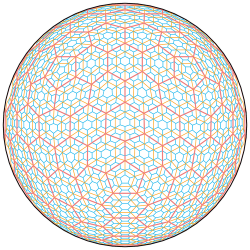
Figure 1. Illustrates the 2nd to 4th level global hexagonal discrete grid generated by DGGRID (Sahr, 2015).

2. Basic idea

This paper aims to explore the performance characteristics of the isotropic hexagonal grid in isoline extraction, highlighting its notable advantages compared to the traditional square grid. We utilize the characteristic of the continuous spatial distribution of the same isoline in the grid space to extract the isoline. The results of this approached are raster images, on which the isolines are rendered. For each grid cell, its’ color is calculated according to the attribute value (Gul & Khan, 2010; Schlei, 2009).

Additionally, when addressing global issues, classic Cartesian grid-based data are becoming inadequate (Breunig et al., 2020; Li et al., 2020). To efficiently analyze these massive volumes of data, it is crucial to provide them in a seamless interoperable format without the need for transformations between different cartographic projections (Baumann, 2021). In addition to its computational cost, reprojecting introduces supplementary artifacts and uncertainties (Kmoch et al., 2022).

Therefore, this paper deploys the isoline algorithm on a globally spherical discretized hexagonal grid. The specific extension steps are as follows: (1) Construct a spherical hexagonal discretized grid; (2) Integrate geographical data on the spherical hexagonal grid; (3) Reclassify the grid cells based on data ranges; (4) Extract the boundaries of the reclassified grid cells; (5) Extract grid isolines on a higher resolution grid; (6) Compare and validate the isoline extraction results with those from a spherical square grid.

3. Constructing spherical hexagonal grid-based data

3.1. Spherical hexagonal grid structure

This study requires the selection of a suitable global hexagonal discretized grid. Firstly, it should possess uniform geometric characteristics. Currently, the construction of a spherical hexagonal discretized grid is primarily based on the regular octahedron (Bai, 2011) or icosahedron (Sahr, 2008; Y. Zhang et al., 2006). Comparatively, the icosahedron is the closest among the regular polyhedral to a spherical shape, which can reduce the deformation during surface mapping between polyhedral and spheres. Hence, this paper opts to construct a global hexagonal discretized grid based on the regular icosahedron.

Secondly, it should be conducive to subdividing this polyhedron to create multiple resolution discrete grid, where the ratio of the areas of a planar polygon cell at resolution k and at resolution k + 1 is referred to as the aperture. Commonly used apertures in hexagonal grid include 3, 4, and 7 (Sahr et al., 2003). For aperture-4, the centerlines of each of the six child units align with the six parent edges. These units maintain consistent orientation across various scales. Aperture-4 offers the advantage of evenly distributing each of the six child units among the parent units (Bousquin, 2021). Therefore, this paper chooses the icosahedral Snyder Equal Area Aperture 4 hexagonal Grid (ISEA4H), Figure 1 (Sahr, 2011).

3.2. Generation of hexagon grid-based data

The data sources used to generate the hexagonal grid include discrete points, TIN, and traditional square grid dataset. The existing values at the centers of TIN or square grid cells are taken as discrete attribute values, and are stored to hexagonal grid cell center. The specific steps are as follows:

1. Select an appropriate grid resolution level based on the research scale and data source resolution.

2. Resample discrete points to hexagonal grid cells center using nearest neighbor interpolation.

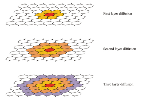
3. For any hexagonal cells without an assigned value, search neighbors in recursive bands until at least four with valid values are identified (Figure 2). Estimate the cell value by utilizing the inverse distance-weighted interpolation method based on the spherical distance formula (Equation 1(1) $\mathrm{S}=\mathrm{R}\ast {cos}^{-1}\left[cos{\beta }_{1}cos{\beta }_{2}cos\left({\alpha }_1-{\alpha }_2\right)+\mathit{\hspace{0.17em}}sin{\beta }_{1}sin{\beta }_2\right]$(1) ).

   (1) $\mathrm{S}=\mathrm{R}\ast {cos}^{-1}\left[cos{\beta }_{1}cos{\beta }_{2}cos\left({\alpha }_1-{\alpha }_2\right)+\mathit{\hspace{0.17em}}sin{\beta }_{1}sin{\beta }_2\right]$(1)

Figure 2. Diffuse query adjacent neighborhood diagram.

4. Extraction of isoline based on hexagonal-gridded structure

The method of isoline extraction stems from the natural characteristics that the same contour is continuously distributed within the space. We start from a grid cell within the study area and conduct a recursive search along the neighborhoods in six directions. By comparing the numerical differences between adjacent grid cells, all interconnected grid cells with the same value range will be connected, forming a complete isoline area.

4.1. Reclassify grid cells

The reclassification algorithm involves grouping interpolated data based on specific conditions, with each group representing a range of values for a contour line. The value range for each category can be defined according to the spatial gradient requirements. For instance, in the isoline of precipitation, grid cells with rainfall between 0 to 3 mm are grouped into one category, those with rainfall between 3 to 6 mm into another, each assigned a category code, and so on. While this classification method may overlook some intermediate contour values in certain locations, failing to accurately represent the detailed distribution of contour lines, it doesn’t significantly impact the expression of macroscopic information distribution, particularly in large-scale regions like the global oceans. Additionally, it helps avoid issues such as isoline intersections during the contour tracing process.

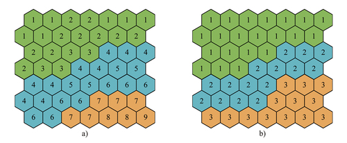
The reclassification algorithm is relatively straightforward; during computation, it iterates through all calculation grid cells once, reassigning values to the grid cells based on specified reclassification conditions. Figure 3a) depicts the numerical values of the grid cells after interpolation, where each number represents the precipitation value for each grid cell. Figure 3b) illustrates the grid values after reclassification, with the numbers indicating the category to which each grid cell belongs. Grid points within the same category represent grid cells with similar value ranges. It is evident from 3b) that the continuous region formed by all grid cells within the same category constitutes a contour area.

Figure 3. Reclassifying interpolated data, a) Interpolated data; b) Reclassified data.

4.2. Trace isoline boundaries

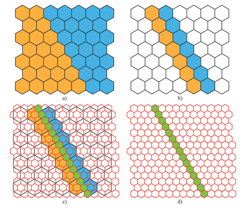
This paper utilizes the flood fill algorithm to derive contiguous grid regions of the same classification. Subsequently, isoline are traced by extracting the boundaries of these grid regions. It concludes the following steps (Figure 4):

1. Flood fill Algorithm: Choose an appropriate grid cell and employ the flood fill algorithm by evaluating concentric rings of hexagons centered on the starting cell to obtain grid regions of the same classification that are contiguous. Simultaneously, mark the searched grid cells to avoid duplication until no further growth is possible.

2. Grid Region Boundary Extraction: Within each category, traverse each grid cell. Based on whether adjacent grid cells categories are the same, extract the outer grid cells of each region to delineate contour boundaries.

3. Isoline Tracing: Get cell boundaries at a higher resolution grid through the common edges of different regions.

Figure 4. The algorithm of tracing isoline, a) Use flood fill algorithm to set same classification grid cells with same value; b) Extract the outer grid cells of each region; c) Query outer grid cells in higher resolution grid; d) a traced isoline.

5. Case study

In order to assess the isotropic properties of spherical hexagonal grid in extracting isoline from global geographical data, this study conducted a comparative validation with traditional square grid. The square grid is structured as a Gaussian latitude-longitude grid, wherein latitude lines extend from −90 degrees to 90 degrees and run parallel to one another, while longitude lines span from −180 degrees to 180 degrees, also in parallel alignment. These lines share uniform angular increments. The square grid is delineated by the intersecting latitude and longitude lines, where the enclosed areas between adjacent lines form the individual grid cells.

To ensure the fairness of the experiment, we set the resolution of the spherical square grid equal to the resolution of the hexagonal grid at the equator. Utilizing the identical data source and following the procedures outlined in Section 3.2, values were interpolated onto grid cells of both types. Subsequently, isoline were extracted following the methods outlined in Section 4, with the only difference being the neighborhood quantity—6 neighborhoods for hexagonal grid and 8 neighborhoods for square grid.

5.1. Data source

Sea surface temperature (SST) is a key determinant in the interaction between the ocean and the atmosphere, as well as in climate change (Wentz et al., 2000). SST also plays a significant role in the development and evolution of tropical storms and hurricanes (DeMaria & Kaplan, 1994; Emanuel, 1999), is correlated with nutrient concentration and primary productivity, and affects the distribution of fishing grounds (Q. Q. Shao et al., 2007). Therefore, sea surface temperature is a crucial data source in geographic spatial data.

The Physical Sciences Laboratory (PSL) of the National Oceanic and Atmospheric Administration (NOAA) in the United States provides numerous high-quality, high-resolution datasets for research in the fields of oceanography and atmospheric science. For this study, the primary data source was the COBE-SST global sea surface temperature dataset compiled by the Japan Meteorological Agency (JMA), which was obtained by downloading it from the NOAA Physical Sciences Laboratory (PSL) in Boulder, Colorado, USA. The dataset was accessed through their website at https://psl.noaa.gov. This dataset comprises global ocean grid square data with a spatial resolution of 1° × 1°, providing monthly averages with a time range extending from January 1891 to the present. The data is formatted in NetCDF. An example SST map is presented in Figure 5.

Figure 5. Example output map of SST for January 2021.

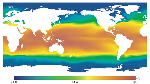
This study utilizes the average sea surface temperature for the month of January 2020 as the focus of investigation. The average sea surface temperature in January ranges from −1.8°C to 31.2°C. With 0°C designated as the starting contour line and a contour interval of 5°C, the sea surface temperature range is classified into 8 classes using the algorithm outlined in Section 4.1. Each class is assigned a category code ranging from 0 to 7, and the specific classification results are illustrated in Figure 6.

Figure 6. Value classification algorithm.

In order to ensure that the sampling density of the tessellation models for hexagonal and square grid is the same, the resolution of the square grid is kept consistent with the resolution at the equator for the hexagonal grid. Table 1 displays the grid resolutions of spherical hexagonal grid at levels 5 to 8 and the corresponding resolutions for spherical square grid.

Table 1. The resolution information of hexagonal and Square Grid.

Resolution of two types of grid
Level	5	6	7	8
Hexagon	1.96° x 1.96°	0.98° x 0.98°	0.49° x 0.49°	0.25° x 0.25°
Square	2° x 2°	1° x 1°	0.5° x 0.5°	0.25° x 0.25°

5.2. Comparison of reclassified grid

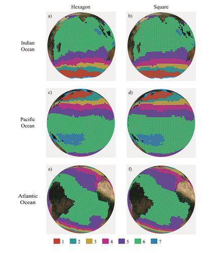
In this study, we compared the classification of three ocean region using spherical hexagonal and square grid at resolution of level 5. To assess the sensitivity of isoline to grid geometry, we categorize the data with a contour interval of 5 (as Figure 6). From a visualization perspective, as shown in Figure 7, where a), c), and e) represent the classification results of hexagonal grid on three oceans, and b), d), and f) represent the classification results of square grid on three oceans. It is not difficult to observe that, for each region the results are similar. It is not difficult to see that, at the same resolution, the hexagonal grid exhibits clearer and smoother boundary contours in different classified areas compared to the square grid. More specifically, for illustrative purposes, consider the example in the Indian Ocean region at the boundaries between categories 5 and 6. It becomes apparent that hexagonal grid offers a more detailed representation of contour lines, while those drawn by square grid appear rigid.

Figure 7. The comparison of grid classification with hexagon and square grid at level 5 for three ocean regions.

5.3. Comparison of extracted of isoline

Based on reclassified grid cells with both hexagons and squares under varying resolutions in Section 5.2, the isoline are extracted by the 6 neighborhoods and 8 neighborhoods algorithms following the extraction steps mentioned earlier. We assessed the effectiveness in isoline extraction between the hexagon grid and the square grid from ocean data by means of visual and quantitative.

5.3.1. Visual comparison

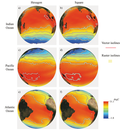
This method directly evaluates the performance of hexagonal and traditional square grid by overlaying vector isoline onto the raster isoline extracted from both grid types. Figure 8 illustrates the overlay results in the three ocean region for hexagonal and square grid, where a), c), and e) represent the overlay results of hexagonal grid on three oceans, and b), d), and f) represent the overlay results of square grid on three oceans. The comparative results across the three oceanic regions reveal slight deviations in the isoline extracted by both grid types compared to the vector lines. Despite these differences, the results based on hexagonal grid demonstrate greater consistency than square grid, showcasing outstanding performance in preserving curved characteristics. This suggests that at the same resolution, hexagonal grid exhibit a more significant advantage in maintaining both location accuracy and curved features.

Figure 8. The isoline extraction based on hexagonal and square grid in three ocean area under level 6.

To further elaborate on this advantage, Figure 9 provides a closer, more detailed view. The distinction becomes evident as the isoline extracted by square grid exhibit corners with angles close to 90°, whereas those extracted by hexagonal grid display corners with angles of 120°. Notably, the deviation of extraction results from vector lines is more pronounced in the case of square grid compared to hexagonal grid.

Figure 9. Zoom in details of isoline based on hexagonal and square grid.

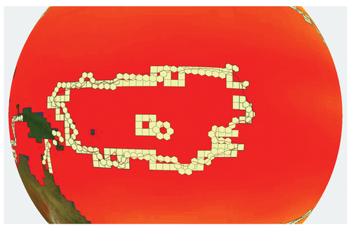
This observation leads to the conclusion that contour lines extracted based on hexagonal grid offer a smoother representation, and to some extent, they preserve curvature more effectively than those extracted by square grid. The distinct corner angles and reduced deviation from vector lines in hexagonal grid-based isoline contribute to a visually appealing and more accurate portrayal of geographic features.

5.3.2. Quantitative comparison

In this approach, the classification results of grid data largely determine the accuracy of contour line extraction. The detailed classification process described in Section 4.1 directly influences the final presentation of isolines. The classification accuracy under different grid configurations becomes a crucial factor, as it represents the ability to describe geographical features at various spatial resolutions. Higher classification accuracy implies a more accurate capture of details and features in geographical data, thereby enhancing the precision of isoline extraction. Therefore, the classification results of grid data not only establish the foundation for the isoline extraction process but also directly impact the reliability and accuracy of subsequent spatial analyses.

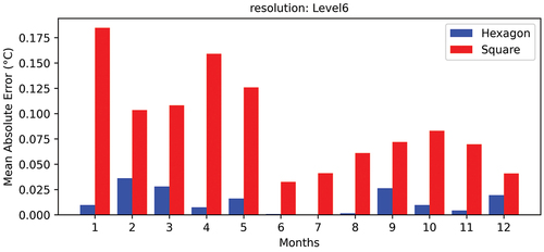
To evaluate the performance of the two grid types in extracting isoline from global sea surface temperature, the Mean Absolute Error (MAE) was computed by comparing the classified values of the grid at level 6 with the interpolated grid values. In theory, a smaller MAE indicates a higher accuracy in aligning the classification of grid cells with the true values. The calculation formula is as follows:

(2) $\mathrm{MAE}=\mathit{\hspace{0.17em}}\frac{1}{N}\sum _{\mathit{i}=1}^N\left|\mathit{Clas}{s}_i-\mathit{\hspace{0.17em}}\mathit{Valu}{e}_i\right|$(2)

Here, N represents the total number of grid cells, $\mathit{Clas}{s}_i$ is the classified value of the grid cell at position i, and $\mathit{Valu}{e}_i$is the interpolated grid value at position i. In order to enhance the accuracy of the statistical results, this study utilizes the monthly average SST from January to December 2020 as the validation data.

Figure 10 compares the Mean Absolute Error (MAE) values of the two grid types for each month. The horizontal axis represents the months, and the vertical axis represents the MAE values. The red bars represent the spherical square grid, while the blue bars represent the spherical hexagonal grid. Firstly, it is evident from the graph that both square and hexagonal grid classification errors are relatively low, with temperature deviations below 0.2°C. This demonstrates that the classification criteria in this study are suitable for global sea surface temperature data. Secondly, regardless of the grid resolution, the MAE values for the spherical hexagonal grid are consistently smaller than those for the spherical square grid, indicating the superiority of the hexagonal grid in classification accuracy.

Figure 10. Comparison of MAE values between square and hexagonal grid.

6. Discussions

6.1. Discussion on different grid levels

Figures 11 and 12 provide a comprehensive view of the classification and isoline extraction outcomes in the Indian Ocean region, obtained through the hexagon-based and square -based methods across various resolutions. Examining Figure 11, it’s noteworthy that at lower resolutions, the hexagonal grid exhibits a notable advantage, presenting clearer and smoother boundary contours in diverse classified areas compared to the square grid. This advantage becomes more pronounced as the resolution increases, showcasing the hexagonal grid’s efficacy in revealing intricate terrain features.

Figure 11. Discussion of grid classification results using hexagon and square grid at different resolutions in the Indian Ocean region.

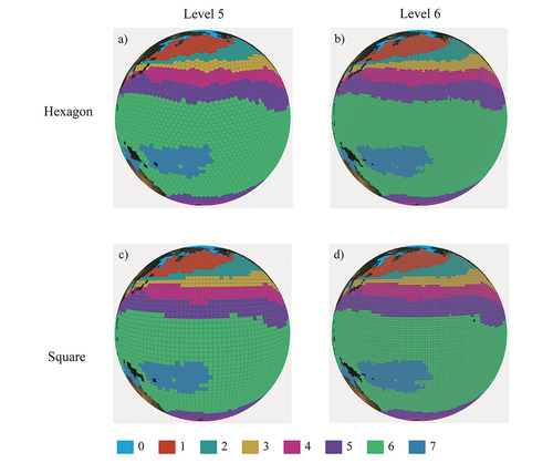
Figure 12. Discussion of isoline extraction results using hexagon and square grid at different resolutions in the Indian Ocean region.

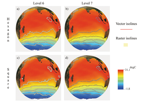
Moving on to Figure 12, illustrating the overlay results for hexagonal and square grid in the Indian Ocean region, a clear trend emerges with increasing resolution. Both grid types exhibit smoother extraction results, demonstrating an enhanced alignment with vector lines. This observation emphasizes the pivotal role of grid resolution in influencing extraction outcomes, underscoring its significance whether dealing with hexagonal or square grid data. The results not only provide insights into the performance of these methods but also highlight the importance of carefully considering resolution in geographic analyses utilizing different grid types.

6.2. Discussion on the 4 and 8 neighborhood of square in isoline extraction

This article demonstrates the impact of the geometric shapes of grid cells on isoline extraction by comparing the results of isoline extraction based on a hexagonal grid with a six-neighborhood and a square grid with an eight-neighborhood. Similar to the approach in Section 5.3.3, we contrasted the effects of orthogonal and diagonal neighborhoods on contour extraction.

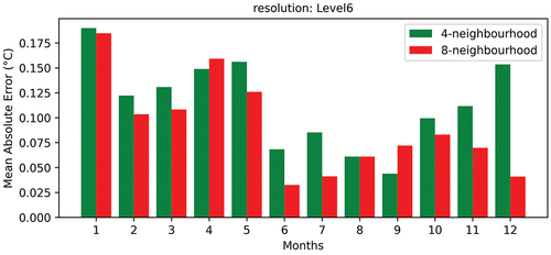
In Figure 13 compares the Mean Absolute Error (MAE) values of the two different neighborhood extraction methods in 12 months. The red bars represent the 8-neighborhood, while the green bars represent the 4-neighborhood. From the figure, it can be seen that, except for the months of April and September, in the other data, the classification error under the eight-neighborhood is smaller than that under the four-neighborhood. This is because the eight-neighborhood provides more spatial information and contextual relationships, resulting in more accurate contour extraction. The 8-neighborhood considers adjacent cells in both orthogonal and diagonal directions, allowing for a more comprehensive capture of geographical features. In contrast, the 4-neighborhood only considers adjacent cells in the orthogonal direction, which may lead to a less comprehensive understanding of geographical structures and, consequently, larger classification errors. Overall, in this context, the eight-neighborhood performs better, enhancing the accuracy of contour extraction.

Figure 13. Comparison of MAE values between 4 neighborhoods and 8 neighborhoods.

6.3. Discussion on the method’s performance

To further evaluate the method’s performance, we applied it to ocean surface elevation data. The dataset selected comprises altimeter satellite gridded Sea Level Anomalies (SLA) computed relative to a twenty-year [1993, 2012] mean. The SLA is determined using Optimal Interpolation, integrating along-track measurements from various available altimeter missions. The dataset was accessed through their website at https://doi.org/10.48670/moi-00149.

Figure 14. Comparison of MAE values between square and hexagonal grid based on SLA data.

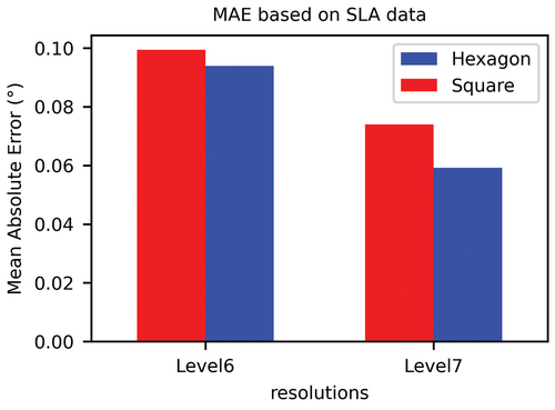
The dataset provides a spatial resolution of 0.25 × 0.25 degrees and a temporal resolution of daily. We randomly selected data from 1 January 2023, and compared the MAE values between two types of grid at different resolutions, as illustrated in Figure 14. The horizontal axis represents the grid resolution, and the vertical axis represents the MAE values. The red bars represent the spherical square grid, while the blue bars represent the spherical hexagonal grid. From the graph, it can be observed that both types of grids exhibit relatively small classification errors, each not exceeding 0.1 m. However, regardless of whether it is at the level 6 grid or a higher resolution grid, the classification error of the square grid is consistently greater than that of the hexagonal grid. Meanwhile, similar to the discussion in Section 6.1, increasing the grid resolution can improve classification accuracy. The accuracy of classification results directly impacts the precision of isoline extraction. Through quantitative comparative experiments on the two datasets, it can be concluded that the isotropic characteristics of the hexagonal grid is well-suited for the integration and analysis of spatial data.

7. Conclusions

The extraction of isoline from grid-based data source may be influenced by the neighborhood relationships among the grid cells. Based on spherical square grid, the inherent differences in distance measurements among the eight directions may result in insufficient isotropy, potentially impacting the extraction of contour lines. Contrastingly, in hexagonal grid systems, they demonstrate superior performance thanks to their consistent connectivity, compact structure, isotropy in local neighborhoods, and visual advantages. Therefore, this article proposes a hexagon-based method for extracting isoline from global Ocean data.

In applying this method to two different types of dataset to test its effectiveness. Comparisons were made with methods based on spherical square structures, leading to the following conclusions. Firstly, hexagonal grid demonstrates superior capability in maintaining positional accuracy and shape features at coarser resolutions. As the resolution decreases, the extracted isoline from both grid types become simplified, but the shape loss in hexagons is not prominent. Secondly, hexagonal grid has an advantage in data classification compared to square grid. Whether at low or high resolutions, the classification accuracy based on hexagonal grid is superior to that of square grid. This further demonstrates that the accuracy of isoline extraction from grid data based on hexagons is superior to that from square grid data. Thirdly, this paper demonstrates the significant impact of grid geometry on the quality of contour lines obtained from grid-based geographical spatial data, providing new insights for spatial analysis of geographical data. Considering the advantages of geographical data spatial analysis based on hexagonal grid, future research will focus on two aspects: (1) Extending this method to extract isoline or feature lines from other global geographical data or different types of geographical data; (2) Performing additional overlay analysis and spatial analysis by integrating the contour lines extracted based on the global hexagonal grid with other data integrated on the grid.

Acknowledgments

The authors express their gratitude to both the editors and anonymous reviewers for their insightful suggestions.

Disclosure statement

No potential conflict of interest was reported by the author(s).

Data availability statement

The dataset is available at https://doi.org/10.5281/zenodo.10574023.

Additional information

Funding

This work was supported by the National Natural Science Foundation of China [Grant no. 42076203].

References

- Ai, T., & Li, J. (2010). A DEM generalization by minor valley branch detection and grid filling. ISPRS Journal of Photogrammetry and Remote Sensing, 65(2), 198–207. https://doi.org/10.1016/j.isprsjprs.2009.11.001
- Amiri, M.-A., Harrison, E., & Samavati, F. (2015). Hexagonal connectivity maps for digital earth. International Journal of Digital Earth, 8(9), 750–769. https://doi.org/10.1080/17538947.2014.927597
- Bai, J. (2011). Location coding and indexing aperture 4 hexagonal discrete global grid based on octahedron. Journal of Remote Sensing, 15(6), 1125–1137. https://doi.org/10.11834/jrs.20110367
- Baumann, P. (2021). A general conceptual framework for multi-dimensional spatio-temporal data sets. Environmental Modelling & Software, 143, 105096. https://doi.org/10.1016/j.envsoft.2021.105096
- Bousquin, J. (2021). Discrete global grid systems as scalable geospatial frameworks for characterizing coastal environments. Environmental Modelling & Software, 146, 105210. https://doi.org/10.1016/j.envsoft.2021.105210
- Breunig, M., Bradley, P. E., Jahn, M., Kuper, P., Mazroob, N., Rösch, N., Al-Doori, M., Stefanakis, E., & Jadidi, M. (2020). Geospatial data management research: Progress and future directions. ISPRS International Journal of Geo-Information, 9(2), 95. https://doi.org/10.3390/ijgi9020095
- Cao, M., Zhang, F., Du, Z., & Liu, R. (2016). A parallel approach for contour extraction based on cuda platform. International Journal of Simulation Systems, Science & Technology, 17,1.1–1.5. https://doi.org/10.5013/IJSSST.a.17.19.01
- DeMaria, M., & Kaplan, J. (1994). Sea surface temperature and the maximum intensity of Atlantic tropical cyclones. Journal of Climate, 7(9), 1324–1334. https://doi.org/10.1175/1520-0442(1994)007<1324:SSTATM>2.0.CO;2
- De Sousa, L., Nery, F., Sousa, R., & Matos, J. (2006). Assessing the accuracy of hexagonal versus square tilled grids in preserving DEM surface flow directions. In M. Caetano & M. Painho (Eds.), Proceedings of ACCURACY 2006 - 7th International Symposium on Spatial Accuracy Assessment in Natural Resources and Environmental Sciences (pp. 191–200). Instituto Geográfico Português.
- Emanuel, K. A. (1999). Thermodynamic control of hurricane intensity. Nature, 401(6754), 665–669. https://doi.org/10.1038/44326
- Gul, S., & Khan, M. F. (2010). Automatic extraction of contour lines from topographic maps. In J. Zhang, C. Shen, G. Geers, & Q. Wu (Eds.), Proceedings of the 2010 International Conference on Digital Image Computing: Techniques and Applications (pp. 593–598). IEEE.
- Jenson, S. K., & Domingue, J. O. (1988). Extracting topographic structure from digital elevation data for geographic information system analysis. Photogrammetric Engineering and Remote Sensing, 54(11), 1593–1600. https://pubs.usgs.gov/publication/70142175
- Jingchang, Z., Runcai, B., Guangwei, L., & Wei, L. (2014). Fast isolines generation algorithm based on TIN. Computer Engineering and Applications, 50(24), 10–15. http://cea.ceaj.org/EN/abstract/abstract32672.shtml
- Keeling, M. (1999). Spatial models of interacting populations. In J. McGlade (Ed.), Advanced ecological theory (pp. 64–99). Wiley. https://onlinelibrary.wiley.com/doi/abs/10.1002/9781444311501.ch3
- Kmoch, A., Vasilyev, I., Virro, H., & Uuemaa, E. (2022). Area and shape distortions in open-source discrete global grid systems. Big Earth Data, 6(3), 256–275. https://doi.org/10.1080/20964471.2022.2094926
- Kreft, J.-U., Booth, G., & Wimpenny, J. W. T. (1998). BacSim, a simulator for individual-based modelling of bacterial colony growth. Microbiology (Reading, England), 144(12), 3275–3287. https://doi.org/10.1099/00221287-144-12-3275
- Liao, C., Tesfa, T., Duan, Z., & Leung, L. R. (2020). Watershed delineation on a hexagonal mesh grid. Environmental Modelling & Software, 128, 104702. https://doi.org/10.1016/j.envsoft.2020.104702
- Li, Z., Gui, Z., Hofer, B., Li, Y., Scheider, S., & Shekhar, S. (2020). Geospatial information processing technologies. In H. Guo, M. F. Goodchild, & A. Annoni (Eds.), Manual of digital earth (pp. 191–227). Springer. https://doi.org/10.1007/978-981-32-9915-3_6
- Liow, Y.-T. (1991). A contour tracing algorithm that preserves common boundaries between regions. CVGIP: Image Understanding, 53(3), 313–321. https://doi.org/10.1016/1049-9660(91)90019-L
- Lu, W., & Tinghua, A. I. (2019). The valley extraction based on the hexagonal grid-based DEM. Acta Geodaetica et Cartographica Sinica, 48(6), 780. https://doi.org/10.11947/j.AGCS.2019.20180408
- Pradhan, R., Kumar, S., Agarwal, R., Pradhan, M. P., & Ghose, M. K. (2010). Contour line tracing algorithm for digital topographic maps. International Journal of Image Processing, 4(2), 156–163. https://scholar.google.com/scholar?cluster=10026589509837249999
- Raposo, P. (2013). Scale-specific automated line simplification by vertex clustering on a hexagonal tessellation. Cartography and Geographic Information Science, 40(5), 427–443. https://doi.org/10.1080/15230406.2013.803707
- Sahr, K. (2008). Location coding on icosahedral aperture 3 hexagon discrete global grids. Computers, Environment and Urban Systems, 32(3), 174–187. https://doi.org/10.1016/j.compenvurbsys.2007.11.005
- Sahr, K. (2011). Hexagonal discrete global grid systems for geospatial computing. Archives of Photogrammetry, Cartography and Remote Sensing, 22, 363–376. https://webpages.sou.edu/~sahrk/sqspc/pubs/sahrMMT11us.pdf
- Sahr, K. (2015). Discrete global grid generation software (Version 6.2b). [Computer software]. https://www.discreteglobalgrids.org/software/
- Sahr, K., White, D., & Kimerling, A. J. (2003). Geodesic discrete global grid systems. Cartography and Geographic Information Science, 30(2), 121–134. https://doi.org/10.1559/152304003100011090
- Schlei, B. R. (2009). A new computational framework for 2D shape-enclosing contours. Image and Vision Computing, 27(6), 637–647. https://doi.org/10.1016/j.imavis.2008.06.014
- Seo, J., Chae, S., Shim, J., Kim, D., Cheong, C., & Han, T.-D. (2016). Fast contour-tracing algorithm based on a pixel-following method for image sensors. Sensors, 16(3), 353. https://doi.org/10.3390/s16030353
- Shao, L., Dong, G., Liu, J., Mu, Y., & Guo, P. (2014). Grid sequence algorithm generating contour based on delaunay triangulation [ Paper presentation]. 2014 IEEE International Conference on Mechatronics and Automation, Tianjin, China. https://ieeexplore.ieee.org/document/6886012
- Shao, Q. Q., Rong, K., Ma, W. W., & Chen, Z. Q. (2007). Generating time-series grid data of sea surface temperature from isotherms in the Northwestern Pacific Ocean using coupled interpolation. Deep Sea Research Part I: Oceanographic Research Papers, 54(4), 673–686. https://doi.org/10.1016/j.dsr.2007.01.004
- Tong, X., Ben, J., Wang, Y., Zhang, Y., & Pei, T. (2013). Efficient encoding and spatial operation scheme for aperture 4 hexagonal discrete global grid system. International Journal of Geographical Information Science, 27(5), 898–921. https://doi.org/10.1080/13658816.2012.725474
- Van Kreveld, M. (1996). Efficient methods for isoline extraction from a TIN. International Journal of Geographical Information Systems, 10(5), 523–540. https://doi.org/10.1080/02693799608902095
- Wang, T. (2008). An algorithm for extracting contour lines based on interval tree from grid DEM. Geo-Spatial Information Science, 11(2), 103–106. https://doi.org/10.1007/s11806-008-0029-4
- Wang, L., Ai, T., Shen, Y., & Li, J. (2020). The isotropic organization of DEM structure and extraction of valley lines using hexagonal grid. Transactions in GIS, 24(2), 483–507. https://doi.org/10.1111/tgis.12611
- Wang, J., Qian, C., & Rui, Y. (2007). A practical method for contour generation based on raster data. Science of Surveying & Mapping, 32(6), 88–90. https://chkd.cbpt.cnki.net/WKE2/WebPublication/paperDigest.aspx?paperID=7fba0722-813e-41fb-8566-db1cb2fb5a38
- Wentz, F. J., Gentemann, C., Smith, D., & Chelton, D. (2000). Satellite measurements of sea surface temperature through clouds. Science, 288(5467), 847–850. https://doi.org/10.1126/science.288.5467.847
- Zhang, Y., Ben, J., Tong, X., & Dai, C. (2006). Geospatial information processing method based on spherical hexagon grid system. Journal of Zhengzhou Institute of Surveying and Mapping, 23(2), 110–114. https://api.semanticscholar.org/CorpusID:124306491
- Zhang, M., & Liang, W. (1997). An improved method for contouring on network of triangles. Computer Aided Design and Computer Graphics Journal, 9(5), 213–217. https://cstj.cqvip.com/Qikan/Article/Detail?id=2436180