Spatiotemporal snowmelt patterns within a high Arctic landscape, with implications for flora and fauna

ABSTRACT

Snow conditions are important drivers of the distribution and phenology of Arctic flora and fauna, but the extent and effects of local variation in snowmelt are still inadequately studied. We analyze snowmelt patterns within the Zackenberg valley in northeast Greenland. Drawing on landscape-level snowmelt dates and meteorological data from a central climate station, we model snowmelt trends during 1998–2014. We then use time-lapse photographs to examine consistency in spatiotemporal snowmelt patterns during 2006–2014. Finally, we use monitoring data on arthropods and plants for 1998–2014 to investigate how snowmelt date affects the phenology of Arctic organisms. Despite large interannual variation in snowmelt timing, we find consistency in the relative order of snowmelt among sites within the landscape. With a slight overall advancement in snowmelt during the study period, early melting locations have advanced more than late-melting ones. Individual organism groups differ greatly in how their phenology shifts with snowmelt, with much variance attributable to variation in life history and diet. Overall, we note that local variation in snowmelt patterns may drive important ecological processes, and that more attention should be paid to variability within landscapes. Areas optimal for a given taxon vary between years, thereby creating spatial structure in a seemingly uniform landscape.

KEYWORDS:

• Snowmelt
• spatiotemporal variability
• phenological mismatch
• high Arctic
• climate change

Introduction

While much research on populations, communities, and ecosystem functions at high latitudes has been focused on processes occurring during the summer, the “inactive” period is longer and may have stronger impacts (Lack 1954). Winter is often a critical phase for the survival of animals that remain active year round (Forsman and Mönkkönen 2003; Mosbacher et al. 2016). Indeed, winter conditions can explain species distribution at cross-latitudinal (Hill et al. 2002; Parmesan and Yohe 2003), regional (Heino 2001), and local scales (Avila-Jiménez et al. 2011).

A key element of Arctic winter is snow. The timing of snow cover is currently changing fast, with rapidly progressing climate change. Winter temperatures in the Arctic have risen more than summer temperatures (Walsh 2014). Drastic changes have been observed in a number of parameters associated with snowmelt, such as winter temperatures and precipitation, the extent of ice cover, annual snow cover, episodic melt events in winter (Pedersen et al. 2015), the frequency of rare events (Vikhamar-Schuler et al. 2016), and snowmelt dates (Bokhorst et al. 2016; Callaghan et al. 2011). Overall, the duration of Arctic snow cover is decreasing rapidly (~3–5 days per decade), particularly because of earlier spring melt (20% per decade) and later onset of snow cover (Bokhorst et al. 2016). At the same time, many areas are experiencing increased snowfall (Cohen et al. 2012), which makes the prediction of net changes in the timing of snowmelt difficult. Because of altered precipitation regimes, future snow cover under climate change is expected to become more variable in space and time (Wipf and Rixen 2010).

Topographical variability is the main cause for differences in local-scale snow conditions (Dobrowski 2011). For many sessile or poorly dispersive taxa, such variation may have a major impact on realized distributional and phenological responses, as dictated by the timing of snowmelt, which will affect both when the ground becomes exposed to warming sunlight (Wipf, Stoeckli, and Bebi 2009) and when the cover of snow will stop buffering temperature fluctuations (Inoue 2008). Indeed, plant and insect populations may be strongly affected by small-scale variation (Badik et al. 2015), and the local timing of snowmelt has been proposed to have a major influence on local species occurrence (Leingärtner, Krauss, and Steffan-Dewenter 2014). Yet research on the impact of snow conditions on phenology typically uses average conditions: temperature and snow conditions characterized by either single weather stations for large areas or by longer-term averages across sites (Høye et al. 2014; Iler et al. 2013; Kudo and Ida 2013). Conflicting with such descriptions is the finding that the exact timing of snowmelt will vary in space and time, with spatiotemporal consistency likely affecting consistency in the timing of local phenological events and demographic processes (Bowden et al. 2015b). Yet the exact effect of snowmelt patterns at the plot versus landscape level is rarely considered. Effects of this type are likely particularly important for experimental manipulations of snowmelt or temperature, as small-scale manipulation will alter the position of the plot on the landscape-level snowmelt gradient. This can, in turn, greatly alter, for example, the way a plant interacts with its neighbors (Wipf, Rixen, and Mulder 2006) or with the surrounding pollinator community (Gezon, Inouye, and Irwin 2016).

Plants and arthropods are presumably among the organisms most sensitive to snowmelt. For plants, snowmelt dictates the onset of activity by allowing photosynthesis (Buus-Hinkler et al. 2006) and subsequent flowering, especially in early flowering species (Høye, Ellebjerg, and Philipp 2007a). For arthropods as poikilothermic animals, a warmer temperature not only speeds up development but also increases the metabolic rate during the inactive overwintering phase. Larvae and pupae may then consume their energy reserves and be forced to emerge at a potentially smaller adult size and with reduced fecundity (Bowden et al. 2015a). Of course, the temperatures experienced by hibernating arthropods depend not only on ambient temperatures but also on, for example, the insulating properties of snow, the presence of permafrost, and the overwintering strategy of the given taxa (sheltered versus exposed; Turnock and Fields 2005).

Attesting to the importance of local snowmelt conditions, Høye, Ellebjerg, and Philipp (2007a) found the onset of flowering to be more dependent on the time of snowmelt, with the subsequent duration of flowering being conditional on prevailing temperatures. This view was further supported by the finding that the total landscape-level flowering period in the high Arctic condenses as the mean snowmelt date becomes earlier and summer temperatures rise (Høye et al. 2013). Arthropod phenology in the high Arctic is also heavily influenced by the timing of snowmelt (Høye et al. 2007b), with earlier exposure to higher solar radiation possibly accentuating the effects (Høye et al. 2008). The relative contributions of and possible synergistic effects between advancing snowmelt dates and rising growing-period temperatures are currently unknown, because local snowmelt dynamics remain poorly explored (but see, e.g., Pedersen et al. 2016).

In this study, we take advantage of the long-term monitoring of snow conditions in the Zackenberg Valley of northeast Greenland (zackenberg.dk). To resolve both large-scale patterns in the mean conditions of a well-studied region and finer patterns around this mean, we draw on multiple data sets collected across the valley (Table 1): data on snowmelt trends recorded at the landscape level during 1998–2014; a set of oblique photographs documenting snow-cover conditions across the valley for 2006–2014; and data on arthropods from 1998–2014 reflecting the phenology of multiple organism groups. We ask: How have the mean timing and the landscape-wide spatial pattern of snowmelt changed during the past nine years of monitoring? How are these changes perceived at a local scale of plots used to study arthropod communities and floral phenology? How is the local consistency of conditions within plots affected by yearly variation across the valley: are early plots consistently early and late plots consistently late? To what extent are the plant flowering phenology and the timing of mean occurrence of different arthropod taxa explained by local snowmelt, compared to other environmental variables (most importantly, ambient temperatures at key life stages)? And finally, do life history traits explain which groups of organisms are the most liable to experience shifts in phenology?

Table 1. The type and time span of data sets used in individual analyses. Data are split by the focal question addressed, the variables examined, and the temporal extent of the data. For details, see Appendix, Table A2

Focus of Interest	Type of Data	Variables Included	Temporal Coverage
Spatial patterns in snowmelt	Time-lapse orthophotographs	Snowmelt date for each pixel, pixel position	2006–2014
Long-term trends	Abiotic data recorded at the climate station	Date of 50% ground uncovered, maximum snow depth, temperature sum	1998–2014
Biotic responses	Biotic data from arthropod trapping and plant monitoring. In situ monitored snowmelt dates and other abiotic data recorded at the climate station	50% flowering for six plant species, mean date of occurrence for thirty-eight arthropod taxa, sampling site coordinates, snowmelt date, maximum snow depth, temperature sum, fall soil temperature	1998–2014

Materials and methods

The Zackenberg Valley (74° 30ʹ N, 21° 00ʹ W) is characterized by a high Arctic climate, with monthly average temperatures ranging from −20°C to 7°C and annual precipitation around 260 mm (Hansen et al. 2008). The valley can be divided into a western part, dominated by gneiss and granite bedrock, and an eastern part, dominated by sedimentary and basaltic bedrock. The lowland is dominated by non-calcareous sandy fluvial sediments (Elberling et al. 2008). The vegetation is relatively rich and diverse, with the landscape mainly covered by small shrubs (Bay 1998).

The data sets used in this study, and the time periods covered by individual sets, are summarized in Table 1 and described in further detail in the Appendix, Table A2. Snow conditions within the valley are recorded by a camera rig on top of a boulder, overlooking the valley from the eastern slope of the Zackenberg Mountain (Figure 1; Buus-Hinkler et al. 2006; Hinkler et al. 2002). To minimize influences of camera types, we used only imagery from three similar cameras from the period 2006–2014. The images were orthorectified and georeferenced, after which each pixel on the map corresponds to twenty-five square meters. The open, sloping Zackenberg valley provides an ideal setting for landscape-level analyses, because only a few smaller areas are obscured by topography.

Figure 1. Location of the Zackenberg camera rig, of the instrument measuring snow depth at the main climate mast, and of plots for monitoring arthropod and plant phenology in the Biobasis program (Schmidt et al. 2016a). A single orthorectified photograph from camera two (DoY 169 of 2014) is overlaid on the map under 10 m elevation contours

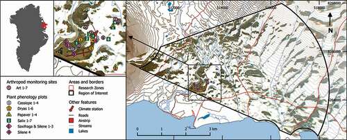
To characterize local snowmelt (Table 1), we focused on images from the snowmelt period from May 1 to July 19. All dates are henceforth given as day of year, with May 1–July 19 corresponding to day of year (DoY) 121–200. During the focal time period, visibility in the valley is sometimes impaired by fog. For days with no visibility, no photographs could be included. Because melt rates are notably lower during foggy conditions (Kankaanpää, personal observation), the missing days were ignored. To account for variable lighting conditions, the photos were batch processed for a maximal tone curve so that the lightest point would be white and the darkest black. Because there are always permanent snow beds and some bare ground (like the station runway, which is cleared from snow early in the spring; Figure 1), this resulted in an accurate scale. The location of permanent snow beds was used as a reference area for fixed white balance, removing the blueness of pictures for the overcast days.

For each pixel, we calculated snowmelt dates using a custom R-script, performing the following steps: the snow situation of each day was turned into a spatial true-false matrix by assigning pixels with all color-channel (RGB) values greater than 210 as true for snow. These matrices were then compared to the situation on the previous day and the DoY. The first DoY when the ground was visible for each pixel of the raster map was then written into a new matrix as the date of snowmelt. This was done for each pixel in each of the available years (2006–2014). We further explored the resulting nine-layered raster stacks of yearly snowmelt date maps by calculating trends and correlations with mean values for each pixel separately. All scripts used are available on request from the first author.

To understand the main factors determining the mean snowmelt timing in Zackenberg we used a multiple linear regression model to tease apart the contributions of snowfall and temperature. For this separate analysis we used the full Zackenberg climate data (Table 1) available from 1996 (or 1998) onward (depending on the type of the data, see Table A1 in the Appendix for full details). The response variable, snowmelt date, was interpolated from snow depletion data (available in the Greenland Ecosystem Monitoring database, http://data.g-e-m.dk/, and on request from K. Skov or M. Lund for 2003–2005) to interpolate dates of 50 percent snow cover. These data match well with the numbers extracted from our spatially explicit maps (Appendix, Figure A2), a finding that acts as an independent validation. This is in line with the accuracy of other similar approaches (Macander et al. 2015). As covariates we used maximum snow depth recorded at the weather station, May–July average temperature, and temperature sums (defined as the sum of daily mean temperatures above zero during the first 200 days of the year).

To establish how landscape-level patterns are reflected at a scale typically used in ecological studies, we focused on pixels around the permanent plots used for monitoring plant phenology and arthropod phenology and community composition within the valley (Schmidt et al. 2016a; Figure 1, Table 1). Here, the reproductive phenology (flowering) is recorded for Cassiope tetragona (four plots), Dryas spp. (six plots), Papaver radicatum (four plots), Salix arctica (seven plots), Saxifraga oppositifolia (three plots), and Silene acaulis (four plots) on a weekly basis during the growing season (late May through early September). The plots range in size from 1 m × 1 m (Silene 4) to 15 m × 20 m (Salix 2), with variation in size scaled to variation in flower densities.

Comparative, systematic sampling of arthropod abundances is carried out by means of yellow pitfall traps placed in five different plant communities (Art 2–5 and 7; Figure 1, Table 1), forming a habitat gradient from wet fen (Art 2) to arid heath (Art 5 and 7), and window traps at a single pond-side location (Art 1). A further plot, Art 6, is situated in a lower terrain with late-laying snow. The monitoring of this site was discontinued in 1999, and it is thus omitted from our analysis of phenological responses. Each pitfall trapping site is made up of four 5 m × 5 m squares, in which the locations of four pitfall traps are randomized each year. The traps are emptied on a weekly basis throughout the summer season. Arthropods are sorted into taxonomic groups (ranging from the order to the species level; see Appendix, Table A3), counted, and preserved at the Museum of Natural History, Aarhus.

For the individual sampling plots, we used the snowmelt photographs to examine how they vary between years in terms of their melt order and melt timing in relation to the global mean melting values averaged across the valley (Table 1). For these monitoring plots, we included twenty-one pixels, which translates to 525 m² in the field—an area comparative to the 5 m × 20 m sampling plots. We then moved on to analyzing what this implies in terms of organismal responses. Phenology within these plots have previously been analyzed in relation to climatic variation, but then characterized by temperature or snow cover at the single weather station in the middle of the valley (Høye et al. 2008, 2013). In other cases (Høye and Forchhammer 2008), the analyses have built on a considerably shorter time series than examined here. We specifically analyzed the role of local variation in the timing of snowmelt, together with other more commonly explored environmental variables including air and soil temperature.

To achieve a deeper understanding of plant and arthropod responses to local snow conditions, we applied a hierarchical joint species distribution model (Ovaskainen et al. 2016). This allowed us to simultaneously model the impact of environmental variables, species-specific traits, and the spatiotemporal context of the data. Using this framework, we aimed to estimate how much of the variation in species phenologies can be explained by the temporal variation in local snow conditions, and whether different groups of taxa and guilds differed in their responses. For this, we used two taxon-specific phenological metrics as our response data: the dates when 50 percent of flowers were open and the mean dates of occurrence for arthropods (calculated as [sum of individuals per trap-day] × [DoY of trap collection] / [sum of individuals per trap day]). These data consist of six plant species (Cassiope tetragona, Dryas octopela x integrifolia, Papaver radicatum, Salix arctica, Saxifraga oppositifolia, and Silene acaulis) from twenty sampling sites, and of window or pitfall trap data on forty-four arthropod taxa. The latter forty-four taxa were selected to be organisms identified to the family level (cf. Schmidt et al. 2016a) and represented by a large enough sample size (see Appendix, Table A3) from six sampling sites in varying habitats (Figure 1; see Schmidt et al. 2016a; also note that monitoring of Art 6 was discontinued in 1999 and is not included in the analysis).

In each plot and year, arthropod sampling has begun when the plots are revealed from under the snow, resulting in some variation in time of initiation between years. Yet the early catches are modest in comparison to peak season, and will thus have only a minor impact on our metric of mean occurrence. In terms of the end of sampling, variation in the extent to which the monitoring has continued into the autumn results in variation in the late-season records. For this reason, we truncated the data at DoY 238, to make the data comparable between years. We modeled the data assuming a normal distribution. As continuous environmental covariates, we included snowmelt date (and its square term) recorded on site (i.e., in the sampling plot), soil mean temperature during fall months (as recorded at the central climate tower), and temperature sums (above-zero degree days during the first 200 days; also recorded at the climate tower). To account for the spatial nature of the data, we considered the identity of the plots as a random effect. As a second random effect, we included year, which handles interannual fluctuation. Because we were interested in assessing the effect of time on the phenology of plant and arthropod communities, we also included year as a fixed, continuous effect, thus capturing linear trends throughout time. Detailed information on data-collection procedures is available in Schmidt et al. (2016a) and yearly summaries can be found in the Zackenberg Ecological Research Operations (ZERO) annual reports (zackenberg.dk/publications/annual-reports/). To make use of the full Zackenberg arthropod and plant phenology time series for our community analyses, we used snowmelt timing data available for the seventeen-year period (Table 1). To characterize the timing of snowmelt at the level of the local sampling plot, we used in situ observations at sampling sites (from ZERO annual reports).

To assess the effect of taxon-specific traits on phenological responses, we also included trait data in the models (seven categories; i.e., autotrophs, detritivores, flower visitors, herbivores, typically non-feeding adults, predators, and groups including species with very diverse lifestyles). A full table of trait assignments can be found in the Appendix (Table A3). We assessed the influence of the environmental covariates and traits measured on the phenological responses by the variance partitioning approach described in Ovaskainen et al. (2016). Finally, to illustrate the impact of variation in snowmelt dates on realized community-wide phenology, we used the fitted joint species distribution model to predict the phenological changes resulting from hypothetical scenarios of different snowmelt dates. The first scenario consisted of early snowmelt dates, and the second one of late snowmelt dates, defined as the 10 percent and 90 percent quantiles, respectively, of the distribution of snowmelt dates in the empirical data. For the sake of comparison, we constructed a reference baseline scenario in which the snowmelt date was set to the mean value in the data. In all scenarios, we set all the other covariates except snowmelt date to their mean value.

Results

How have mean conditions changed during seventeen years of monitoring?

In the high Arctic, climatic conditions differ strongly even in consecutive years. This is revealed by pronounced interannual variation in snowmelt: at about an average snowmelt date of June 18 (DoY 169), the range seen in yearly mean snowmelt dates was approximately thirty-eight days; that is, more than a month. The size of this variation should be compared to the absolute length of snow-free conditions, spanning a total of only some ninety-nine days (mean of 2006–2009). Against this background of large variation, we find less of a trend during the nine years of the study period. Where the first ten years of operation of the Zackenberg research station (1995–2006) were characterized by a period of rapid warming (associated with a positive Atlantic Multi-decadal Oscillations [AMO] anomaly during the period; Abermann et al. 2017), the following years (2006–2014) showed less of a clear warming trend (Figure 2). Thus, given the background of large variation in snowmelt between years, we observe no significant trend in the yearly means of snowmelt dates during the time period included in our spatially explicit analyses (Figure 4A).

Figure 2. Temporal trends in (A) landscape level snowmelt date, as determined by 50 percent of land area uncovered, (B) maximum winter snow depth as measured at the snow depth mast next to the central climate station, and (C) above-zero degree days for spring and early summer (DoY ≥ 200)

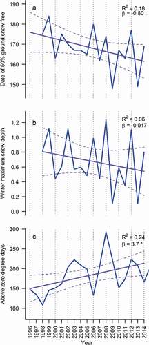
Figure 3. Variation in snowmelt dates (A) among sites and (B) among years within the Zackenberg valley. Panel (A) shows average day of year when the soil at a given site becomes exposed (scale on the right). Panel (B) shows interannual variability, expressed as the standard deviation of the timing of snowmelt (scale on the right). Both panels are based on nine years of data (2006–2014)

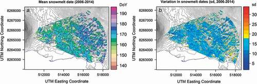
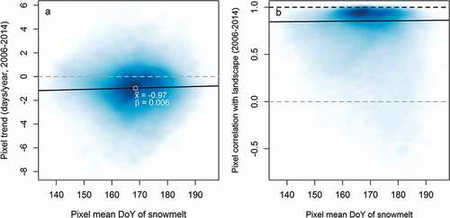
Figure 4. (A) Trend in the timing of snowmelt during 2006–2014 as a function of mean date of snowmelt for any given part (pixel) of the landscape. The average trend is negative, signaling that snowmelt is becoming earlier from year to year. Early melting pixels on average show a steeper trend than late melting sites (black trend line). (B) Scatter plot of average snowmelt pattern of individual pixels (i.e., typical earliness or lateness) and the consistency between mean snowmelt timing at the level of the pixel and the overall landscape (quantified by a correlation coefficient r). Most of the landscape follows the regional snowmelt pattern closely, with a correlation coefficient close to 1, with only a small share of all pixels diverging to a greater extent. Late sites (on the right of the x axis) show the largest variation

During the overall period from 1998 to 2014, the annual mean timing of snowmelt has closely tracked variation in winter snow-depth maxima (Figure 2). In our multiple linear regression model, the observed 1.13 m range in maximum snow depth corresponds to a range of 27.5 days in the timing of snowmelt, with deeper snow packs naturally delaying snowmelt. Variation in snowmelt period temperature, as described by the temperature sum of days above zero, has the opposite effect. A realized range of 184 degree-days translates into a 13.3-day variation in the timing of snowmelt. While no consistent trend can be seen in snow depth over time, the temperature sum for the snowmelt period has been increasing by 3.7 degree-days per year during the past two decades (for complete model summaries, see the Appendix, Table A1).

Is there local consistency in conditions within plots affected by mean conditions: Are early plots consistently early, and late plots consistently late?

Within the Zackenberg Valley, average snowmelt dates vary substantially, with later snowmelt dates being typical for higher altitudes and ravine sides (Figure 3A). Particularly high interannual variability is observed in topographically complex parts of the landscape (e.g., the moraine foothill area in the northern part of the study area; Figure 3B).

Among different areas of the landscape, the pattern of snowmelt is largely consistent among years, with the same areas generally uncovered first every year. Thus, “early sites” do tend to be predictably early and “late sites” tend to be predictably late. Local patterns within most of the landscape seem to follow regional patterns of snowmelt, but for some pixels, local variation bears essentially no resemblance to valley-wide patterns (as revealed by very low correlation coefficients in Figure 4B). Extreme plots at the earliest and latest ends of the continuum showed the highest level of consistency, with some turnover in the timing of snow disappearing from intermediate plots.

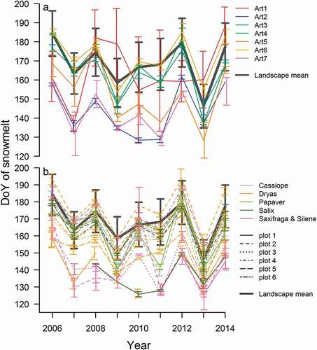
Over time, early melting sites within the landscape have been advancing their snowmelt more than late melting sites. This is illustrated by Figure 4A, where a clear majority of data points (pixels) show a slope below zero in their temporal trend for the 2006–2014 period (i.e., melt earlier over time), and where lower pixel-specific melt days (i.e., earlier sites, to the left on the x axis) show slightly more negative trends over time (i.e., a quicker decrease in DoY at snowmelt). At a small scale, around the plots used to record arthropod communities and flowering phenology, differences in the timing of snowmelt were also large between years. Between the sampling sites monitored for arthropod communities, we see spatial variability of from twenty-five to forty-one days, depending on the year (Figure 5A). Among the plots at the valley floor used to monitor plant flowering, we find interannual variability ranging from thirty-one to forty-four days (Figure 5B).

Figure 5. (A) Yearly snowmelt dates ± 1 standard deviation of the seven arthropod trapping sites situated at the bottom of the Zackenberg valley (see Figure 1). (B) Yearly snowmelt dates ± 1 standard deviation of plant phenology monitoring plots. The mean snowmelt date for the whole valley landscape is plotted for comparison (heavy grey line). Plots named as in Schmidt et al. (2016a) and in Figure 1

What is the role of local snowmelt date in determining plant and arthropod phenologies?

The phenology of plant and arthropod communities was mainly driven by the local snowmelt conditions. The joint species distribution model fitted to the phenological data explained 95 percent of the variation at the plot level, of which most (35%) was explained by the snowmelt date (Figure 6). The impact of snowmelt was particularly marked on the flowering phenology of all the plant species included, and for several key dipteran pollinator taxa such as hover flies (family Syrphidae), muscid flies (Muscidae), dagger flies (Empididae), and some others (Figure 6). In particular, the timing of the flight period of nonbiting midges (Chironomidae) at a given sampling site was almost entirely determined by the timing of local snowmelt (Figure 6), whereas some other taxa seem almost indifferent to plot-level snowmelt date, including dung flies (Scathophagidae) and all diurnal lepidopteran families (Nymphalidae, Lycaenidae, and Pieridae).

Figure 6. Relative proportions of variance in the phenology of plant and arthropod communities attributed to different factors. The variance attributed to the fixed effects is indicated by different shades of blue, whereas the variance attributed to random effects is indicated by different shades of yellow. The taxonomic categories match the original categories of the monitoring data, as here sorted by systematic position (order and class)

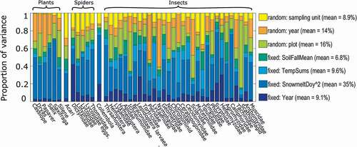
The second most important covariate explaining phenological variation among plants and arthropods was the year. This factor explained 14 percent of the variation as a random effect, and an additional 9.1 percent as a fixed, continuous effect. The latter result indicates that in addition to random variation among years, the phenology of plant and arthropod communities has also changed in a consistent direction throughout the study period. The absolute temperature sum and soil mean temperature during fall months accounted for 9.6 percent and 6.8 percent, respectively, of all variation explained by the model. Early summer temperature sums strongly affect the timing of the flight periods of mosquitoes (Culicidae), diurnal Lepidoptera (Nymphalidae, Lycaenidae, and Pieridae), and the timing of wolf spider reproduction (as reflected by the number of lycosid egg sacks detected). Most random variation (16%) was explained by the plot level, which is no surprise, given that the plots had deliberately been selected to represent different habitat types (see previous).

How the phenology of plant and arthropod taxa responded to different environmental variables seemed largely reflective of their ecology. The diet of the adult phase explained a full 52 percent of the variation observed in responses to the covariates measured.

For all groups except “Herbivores” and “Varied,” different climatic scenarios yielded drastically different phenological patterns at the community level (Table 2). Overall, phenological events occurred significantly earlier under the early snowmelt scenario than under the late snowmelt scenario (Table 2). This was especially the case for “Autotrophs” (plants), for which the predictions between these two scenarios differed by twenty days. Predictions for the baseline scenario (i.e., under current average conditions) showed that of all arthropod taxa, the dietary category including taxa with typically nonfeeding adults occurred earliest in the season, followed by detritivores and predators, whereas groups depending on flower resources and herbivores (which includes larval stages) were active the latest in the season.

Table 2. Predicted phenological occurrences for groups of species with different dietary requirements

Group of Species	Baseline Reference Scenario	Early Snowmelt Dates	Late Snowmelt Dates
Autotrophs	179 (<0.01)	171	191
Detritivores	200 (0.48)	195	209
Flower	207 (>0.99)	199	214
Herbivores	207 (0.96)	206	210
None	192 (0.02)	184	199
Predator	202 (0.91)	196	209
Varied	202 (0.67)	198	205
All	200	193	208

The values in the table show the posterior mean of the predicted phenological date averaged over the species in each group. For all cases expect “Herbivores” and “Varied” (for exact definition, see Appendix, Table A3), the prediction for the early snowmelt date is smaller and the prediction for the late snowmelt date is larger than the prediction for the baseline scenario with >0.99 posterior probability. For “Herbivores” and “Varied,” these posterior probabilities were in the range [0.63 . . . 0.88]. For the baseline scenario, the numbers in brackets show the posterior probability by which the predicted phenological day is larger for the group in question than the average over species.

Discussion

While snow conditions have been identified as important drivers of the distributions and phenologies of Arctic flora and fauna, less is known about the extent and effects of local variation in snowmelt. In the Zackenberg Valley in northeast Greenland, we find that snowmelt has become earlier during the past two decades, with a less clear pattern during the second half of this period. Early snow-free sites are advancing more in terms of their timing of snowmelt, whereas later-melting sites are more variable in their snowmelt schedule. As biotic responses, we see that plants flower earlier with earlier snowmelt, whereas arthropod groups vary substantially in how responsive they are—much of this variation is attributable to taxon-specific life style and diet. In the following section, we will discuss each finding in turn.

Snowmelt patterns across the high Arctic landscape

Although interannual variation in the timing of snowmelt is dramatic in the high Arctic landscape of Zackenberg, the spatial pattern in snowmelt is similar from year to year. Thus, early sites remain early and late sites late; as a consequence, the phenological milieu faced by sessile organisms remains similar. Some substantial variation in snowmelt patterns between years is caused by variation in wind conditions and directions during the winter, causing snow packs to form in different positions (Liston and Sturm 2002; Mernild, Liston, and Hasholt 2007; Pedersen et al. 2016). Rough landscape topography creates areas that differ from mean regional conditions, thus creating local variation within any given year. Thus, even in a generally unfavorable year, parts of the landscape will offer conditions favorable for given animals and plants (Scherrer and Körner 2011). Importantly, this is likely to give rise to spatially structured dynamics in seemingly continuous habitats, where only parts of the population reproduce actively in a given year (Avila-Jiménez et al. 2011; Post et al. 2008). The shifting nature of these so-called nano-refugia may impose a filtering effect on perennial plants and the organisms tightly connected with them. As such sessile organisms are unable to track optimal conditions from year to year by movement, they will have to persist through unfavorable years.

Some interesting effects of phenological shifts are likely to be mediated specifically through the earliest-melting sites, which incidentally also show the largest changes in snowmelt over time. Plants growing at the earliest sites may benefit from limited competition for pollination services (Gezon, Inouye, and Irwin 2016) and enjoy the longest growing seasons, but will at the same time be more exposed to colder temperatures and more frequent freeze-thaw cycles after the initial snowmelt (Gezon, Inouye, and Irwin 2016; Høye et al. 2013; Wheeler et al. 2015; Wipf, Stoeckli, and Bebi 2009). Early and late sites also experience a different mix of radiative energy, soil temperatures, and water availability during their respective growth period, which may in turn alter microbial communities and nutrient availability (Berdanier and Klein 2011; Ernakovich et al. 2014). Thus, early and late melting parts of the landscape are inherently different both in terms of how they are affected by climate change and in the way their communities of organisms are affected by those changes.

Soil temperature is an important factor shaping the biota of arctic landscapes (Hoyle et al. 2013; Sturm et al. 2005) and differentiating Arctic and alpine ecosystems (Ernakovich et al. 2014). Soil temperatures are determined by a complex interplay between ambient temperature, solar radiation, soil type, topographical features (Scherrer and Körner 2010), various aspects of snow cover (Taras, Sturm, and Liston 2002), and the proximity of the permafrost (Hinzman et al. 1991). In the high Arctic, the presence of permafrost further complicates the situation, because it will at times cool the topsoil from below and prevent spring meltwater from draining, thus keeping the topsoil cool and wet after the snow has melted. Thus, depending on the latitude and trends in snowfall, winter soil temperatures are expected to decrease in some areas (Brown and DeGaetano 2011) but increase in others. The possibility has been raised that the north might experience colder winter soil temperatures even with warmer ambient temperatures, because of the loss of insulating snow cover (Brown and DeGaetano 2011; Groffman et al. 2001). Nonetheless, the opposite has also been proposed, based on the biotic feedback mechanism of Arctic shrubification and the snow-retention properties of taller shrubs (Sturm et al. 2005). For our study area, the former hypothesis seems unlikely, because the advancement of snowmelt is mostly the result of rising spring temperatures, while the depth of snow cover has oscillated around a constant mean (Figure 2; Pedersen et al. 2016). Whether the amplitude of these oscillations has increased, or the incidence of extreme, nearly snow-free winters with a strong impact on Arctic biota (Miller and Barry 2009) has grown higher, we cannot conclude based on the data presented here.

Biotic responses to snowmelt patterns

Previous work suggests that different organisms respond differently to changes in snow-cover conditions (Dollery, Hodkinson, and Jónsdóttir 2006; Gauthier et al. 2013) and rising ambient temperatures (Arft et al. 1999; Bjorkman et al. 2015; Cook, Wolkovich, and Parmesan 2012; Gauthier et al. 2013; Hodkinson et al. 1998; Thackeray et al. 2016). Indeed, our analysis of phenological responses of different arthropod taxa reveals striking variation in the imprint of different environmental aspects on different taxa. Which environmental feature proves most influential depends on the general life history of the taxon in question. For some groups encompassing diverse phenological strategies, such as parasitic wasps in family Ichneumonidae, where some species are early and others late (Várkonyi and Roslin 2013), most of the variation gets attributed to the random effect of the sampling plot, because different sites simply host different species assemblages. However, for most other taxa, the families are so species poor in northeast Greenland that this poses no problem. Here, a more phenologically coherent family of parasitoid wasps (Braconidae) shows a phenological dependency structure very similar to that of its main prey item, lepidopteran larvae. Taxa dependent on sporadic (late season) resources such as scat, fungal fruiting bodies, or carrion prove more or less unresponsive to snowmelt pattern, suggesting a stronger response to resources rather than local environmental conditions. A strong imprint of snowmelt date was also observed in the phenological timing of many dipteran pollinator groups, in line with previous studies (Iler et al. 2013). Muscid flies at Zackenberg show a general decline in abundance during the past two decades, but patterns among individual species are highly dissimilar (Loboda et al. 2017). Our species-level data (Wirta et al. 2016) from the area suggest that individual muscid fly species differ substantially in phenology. These differences in phenology could then be linked with demographic trends.

A specific caveat derives from the sampling design employed in Zackenberg biomonitoring (Schmidt et al. 2016a). As the trapping is conducted with yellow pitfall traps (Schmidt et al. 2016a) rather than emergence traps, we cannot separate local processes from the influx of individuals from the surrounding landscape. This may account for why snowmelt date explains more of the phenological variation of soil-borne species such as spiders (Lycosidae, Thomisidae), soil invertebrates (Acari, Collembola), and other poor dispersers (Thysanoptera) as compared to strong fliers such as diurnal Lepidoptera (Nymphalidae, Lycaenidae, Pieridae). In future studies, satisfactory separation of local processes from the inflow of individuals could be achieved by experiments combining terrestrial emergence traps (measuring local recruitment) with passive traps (measuring inflow of individuals).

Community phenology in a changing Arctic

The potential for phenological mismatches between interacting functional groups, such as pollinators or plant feeders, and their predators has caused much concern during the past decade (Jones and Cresswell 2010; Kudo and Ida 2013; Memmott et al. 2007; Miller-Rushing et al. 2010; Post et al. 2008; Saino et al. 2011). From the different responses to snowmelt patterns observed among different taxa (see earlier), we can expect that at least local community composition is liable to change with changes in snow cover. Indeed, our simulations of different snowmelt scenarios suggest drastic differences in the relative phenology of species among years of different timing of snowmelt. At the community level, this will result in completely different patterns of synchrony among community members, and with longer-term change, in shifts in the relative timing of taxon-specific events. How this is reflected in community-level structure, dynamics, and functioning is a salient question in Arctic ecology (Legagneux et al. 2014; Schmidt et al. 2017, 2016b).

Implications for manipulative experiments

Our study reveals substantial variation in local snowmelt patterns, and variable levels of consistency between landscape-level and smaller-scale patterns. Late sites showed the largest variation in consistency with landscape-level patterns. Yet the exact effect of snowmelt patterns at the plot versus landscape level is rarely considered. Variation of this type is likely particularly important for experimental manipulations of snowmelt or temperature, as experimental manipulation of snow cover essentially changes the melting time of the site in relation to the surrounding landscape. As such, this is not always analogous to melt times being regionally altered by large-scale climate change, but can partly elucidate the interplay between the plants and the surrounding pollinator community (Gezon, Inouye, and Irwin 2016) and interactions between neighboring plants (Wipf, Rixen, and Mulder 2006). The limited consistency between patterns at the plot and landscape scale also urges caution when using spatial variation in snow conditions as a surrogate for temporal trends. To eventually assess the effects of climate change on organisms, their interactions, and communities at a landscape level, we suggest that researchers adopt spatial designs that include moderate amounts of variation in snow conditions and record the abiotic phenology on a local scale, while still keeping the landscape mean in their toolbox.

Conclusions

Overall, our study highlights major variability in local snow conditions across space and time in the Arctic. By revealing major differences in how groups of organisms respond to this variation, we add renewed emphasis to its importance. Differential snowmelt in space and time will result in different patterns of community-level phenology, with different levels of synchrony among local community members. These patterns have major implications for the dynamics and functioning of Arctic communities, thus marking snowmelt conditions as a key factor in Arctic ecology. Different phylogenetic and functional groups of organisms also vary greatly in which environmental factors affect their yearly phenology. In particular, species occurring later in the season are less strongly impacted by the timing of snowmelt. Thus, interactions between early and late species may weaken as the onset of spring advances. Given the importance of the timing of snowmelt for organismal phenology and the high geographical variability in winter precipitation trends, global comparisons of phenological changes should, by default, include site-specific snow parameters.

Acknowledgments

We are grateful to Otso Ovaskainen for advice on the application of the HSMC-statistical framework. Data on temperature and snow depth collected by the Greenland Ecosystem Monitoring Program ClimateBasis were provided by Asiaq–Greenland Survey, Nuuk, Greenland. Data on snow cover and organisms of the tundra collected by the Greenland Ecosystem Monitoring Programs GeoBasis and Biobasis were provided by the Department of Bioscience, Aarhus University, Denmark, in collaboration with Department of Geosciences and Natural Resource Management, Copenhagen University, Denmark.

Additional information

Funding

Funding by the Nessling Foundation (to TK), by the Ella and Georg Ehrnrooth Foundation, and by the Academy of Finland (grant no. 276909 to TR) is gratefully acknowledged.

Appendices

Table A1. Multiple linear regression model of snowmelt timing as a function of snow depth and spring temperatures

Multiple linear regression: HalfSnowcoverDoY ~ MaximumSnowDepth + TemperatureSums
	Dependent variable:
	Mean DoY of snowmelt
	coefficient (SE)
Maximum winter snow depth	24.21 (2.64)***
Above zero degree days (DoY 0–200)	–0.07 (0.02)**
Constant	165.14 (4.34)***
Observations	17
R^2	0.87
Adjusted R^2	0.85
Residual Std. Error	3.70 (df = 14)
F Statistic	47.15*** (df = 2; 14)

*p<0.1; **p<0.05; ***p<0.01

Table A2. Data sets used in the analyses included in this article

Analysis	Variable	Description	Manipulation	Years	Source
Spatial patterns of snowmelt	Snowmelt date	Spatially explicit snowmelt dates	First day not covered in snow recorded	2006–2014	Photos from Geobasis
	Vegetation class	Map of vegetation types	Georeferencing		Zackenberg website
Temporal patterns of snowmelt	Snowmelt date	Date of 50% snow cover in the central valley area	Values intrapolated from snow depletion curves. 2003–2005 are based on a slighly different area.	1998–2014	GEM-database, 2003–2005 from Geobasis
	Maximum snow depth	Maximum wintertime snow depth as recorded at a single point	None	1997–2014	Zackenberg annual reports
	Temperature sums	Above zero degree days before 19.7.	Sum of daily means of above 0 for DoY range 0–200	1996–2014	GEM-database: Air temperature (2 m)
Community responses	Arthropod abundancies	Number of individuals per taxon caught with fixed trapping effort. Used to calculate arthropod phenology	Individuals per day per trapping site, period trimmed to end at DoY 235	1996–2014	GEM-database: Arthropod phenology
	Arthropod phenology	Mean DoY of occurrence of arthropod taxa	Sum of individuals per day × DoY of trapping/sum individuals per day, for each trapping site.	1996–2014	GEM-database: Arthropod phenology
	Flower phenology	50% of flowers open	None	1996–2014	Zackenberg annual reports
	Local snowmelt	50% of arthropod/plant plots uncovered from snow	Intrapolated from field observations. Contains inaccuracies at the early end, when the snow has melted before the start of active field season	1996–2014	Zackenberg annual reports
	Autumn soil temperature	Mean soil temperature during previous autumn	Mean soil temperature of August, September, and October	1997–2014	GEM-database: Soil temperature (−5 cm)
	Temperature sums	Above-zero degree days before 19.7.	Sum of daily means of above 0 for DoY range 0–200	1996–2014	GEM-database: Air temperature (2 m)

Table A3. Categories included as traits in the HMSC-analysis. For heterotrophs, the trait value describes adult diet, with "None" referring to typically nonfeeding adults. Flower feeders visit flowers for nectar or pollen resources

Taxon	Adult Diet
Cassiope	Autotroph
Dryas	Autotroph
Papaver	Autotroph
Salix	Autotroph
Saxifraga	Autotroph
Silene	Autotroph
Acari	Detritivore
Dictynidae	Predator
Linyphiidae	Predator
Lycosidae	Predator
Lycosidae egg sack	Predator
Thomisidae	Predator
Collembola	Detritivore
Thysanoptera	Flower
Hemiptera	Herbivore
Lygaeidae	Herbivore
Hymenoptera	Flower
Apidae	Flower
Ichneumonidae	Flower
Braconidae	Flower
Lepidoptera larvae	Herbivore
Tortricidae	Flower
Pieridae	Flower
Lycaenidae	Flower
Nymphalidae	Flower
Geometridae	Flower
Noctuidae	Flower
Chironomidae	None
Culicidae	Varied
Ceratopogonidae	Predator
Cecidomyiidae	None
Sciaridae	None
Mycetophilidae	Flower
Tipulidae	None
Empididae	Predator
Phoridae	Detritivore
Syrphidae	Flower
Heleomyzidae	Varied
Agromyzidae	Flower
Calliphoridae	Flower
Tachinidae	Flower
Scathophagidae	Predator
Anthomyiidae	Detritivore
Muscidae	Flower

Figure A1. Validation of snowmelt data extracted from photographs as compared to ground-truthed observations. Shown are mean snowmelt dates measured from orthophotographs (x axis) and in situ observations of date of 50 percent snow cover (y axis) from the same arthropod and plant phenology plots. The latter includes some values with known uncertainties; that is, cases where the snow of the plot had melted before the first visit. The correlation coefficient (Pearson’s r) between the two is 0.88. The mean difference between mean snowmelt and 50 percent snow cover is 4.7 days

References

- Abermann, J., B. Hansen, M. Lund, S. Wacker, M. Karami, and J. Cappelen. 2017. Hotspots and key periods of Greenland climate change during the past six decades. Ambio 46 (s1):3–11. doi:https://doi.org/10.1007/s13280-016-0861-y.
- Arft, A. A. M., M. D. Walker, J. Gurevitch, J. M. Alatalo, M. Diemer, F. Gugerli, G. H. R. Henry, M. H. Jones, R. D. Hollister, I. S. Jonsdottir, et al. 1999. Responses of Tundra plants to experimental warming: Meta-analysis of the international Tundra experiment. Ecological Monographs 69 (4):491–511.
- Avila-Jiménez, M. L., S. J. Coulson, M. L. Ávila-Jiménez, S. J. Coulson, M. L. Avila-Jiménez, and S. J. Coulson. 2011. Can snow depth be used to predict the distribution of the high Arctic aphid Acyrthosiphon svalbardicum (Hemiptera: Aphididae) on Spitsbergen? BMC Ecology 11 (1). doi:https://doi.org/10.1186/1472-6785-11-25.
- Badik, K. J., A. M. Shapiro, M. M. Bonilla, J. P. Jahner, J. G. Harrison, and M. L. Forister. 2015. Beyond annual and seasonal averages: Using temporal patterns of precipitation to predict butterfly richness across an elevational gradient. Ecological Entomology 40 (5):585–95. doi:https://doi.org/10.1111/een.12228.
- Bay, C. 1998. Vegetation mapping of Zackenberg Valley, Northeast Greenland. Denmark: Danish Polar Center & Botanical Museum, University of Copenhagen.
- Berdanier, A. B., and J. A. Klein. 2011. Growing season length and soil moisture interactively constrain high elevation aboveground net primary production. Ecosystems 14 (6):963–74. doi:https://doi.org/10.1007/s10021-011-9459-1.
- Bjorkman, A. D., S. C. Elmendorf, A. L. Beamish, M. Vellend, and G. H. R. Henry. 2015. Contrasting effects of warming and increased snowfall on Arctic tundra plant phenology over the past two decades. Global Change Biology 21 (12):4651–61. doi:https://doi.org/10.1111/gcb.13051.
- Bokhorst, S., S. H. Pedersen, L. Brucker, O. Anisimov, J. W. Bjerke, R. D. Brown, D. Ehrich, R. L. H. Essery, A. Heilig, S. Ingvander, et al. 2016. Changing Arctic snow cover: A review of recent developments and assessment of future needs for observations, modelling, and impacts. Ambio 45 (5):516–37. doi:https://doi.org/10.1007/s13280-016-0770-0.
- Bowden, J. J., A. Eskildsen, R. R. Hansen, K. Olsen, C. M. Kurle, and T. T. Høye. 2015a. High-Arctic butterflies become smaller with rising temperatures. Biology Letters 11 (10):20150574. doi:https://doi.org/10.1098/rsbl.2015.0574.
- Bowden, J. J., R. R. Hansen, K. Olsen, and T. T. Høye. 2015b. Habitat-specific effects of climate change on a low-mobility Arctic spider species. Polar Biology 38 (4):559–68. doi:https://doi.org/10.1007/s00300-014-1622-7.
- Brown, P. J., and A. T. DeGaetano. 2011. A paradox of cooling winter soil surface temperatures in a warming northeastern United States. Agricultural and Forest Meteorology 151 (7):947–56. doi:https://doi.org/10.1016/j.agrformet.2011.02.014.
- Buus-Hinkler, J., B. U. Hansen, M. P. Tamstorf, and S. B. Pedersen. 2006. Snow-vegetation relations in a High Arctic ecosystem: Inter-annual variability inferred from new monitoring and modeling concepts. Remote Sensing of Environment 105 (3):237–47. doi:https://doi.org/10.1016/j.rse.2006.06.016.
- Callaghan, T. V., M. Johansson, R. D. Brown, P. Y. Groisman, N. Labba, V. Radionov, R. G. Barry, O. N. Bulygina, R. L. H. Essery, D. M. Frolov, et al. 2011. The changing face of arctic snow cover: A synthesis of observed and projected changes. Ambio 40 (S1):17–31. doi:https://doi.org/10.1007/s13280-011-0212-y.
- Cohen, J. L., J. C. Furtado, M. Barlow, V. Alexeev, and J. E. Cherry. 2012. Arctic warming, increasing snow cover and widespread boreal winter cooling. Environmental Research Letters 7 (1):014007. doi:https://doi.org/10.1088/1748-9326/7/1/014007.
- Cook, B. I., E. M. Wolkovich, and C. Parmesan. 2012. Divergent responses to spring and winter warming drive community level flowering trends. Proceedings of the National Academy of Sciences 109 (23):9000–5. doi:https://doi.org/10.1073/pnas.1118364109.
- Dobrowski, S. Z. 2011. A climatic basis for microrefugia: The influence of terrain on climate. Global Change Biology 17 (2):1022–35. doi:https://doi.org/10.1111/j.1365-2486.2010.02263.x.
- Dollery, R., I. D. Hodkinson, and I. S. Jónsdóttir. 2006. Impact of warming and timing of snow melt on soil microarthropod assemblages associated with Dryas-dominated plant communities on Svalbard. Ecography 29 (1):111–19. doi:https://doi.org/10.1111/j.2006.0906-7590.04366.x.
- Elberling, B., M. P. Tamstorf, A. Michelsen, M. F. Arndal, C. Sigsgaard, L. Illeris, C. Bay, B. U. Hansen, T. R. Christensen, and E. S. Hansen. 2008. Soil and plant community: Characteristics and dynamics at Zackenberg. In High-Arctic ecosystem dynamics in a changing climate: Advances in ecological research, edited by H. Meltofte, T. R. Christensen, B. Elberling, M. C. Forchhammer, and M. Rasch, vol. 40, 223–48. London: Elsevier.
- Ernakovich, J. G., K. A. Hopping, A. B. Berdanier, R. T. Simpson, E. J. Kachergis, H. Steltzer, and M. D. Wallenstein. 2014. Predicted responses of arctic and alpine ecosystems to altered seasonality under climate change. Global Change Biology 20 (10):3256–69. doi:https://doi.org/10.1111/gcb.12568.
- Forsman, J. T., and M. Mönkkönen. 2003. The role of climate in limiting European resident bird populations. Journal of Biogeography 30 (1):55–70. doi:https://doi.org/10.1046/j.1365-2699.2003.00812.x.
- Gauthier, G., J. Bety, M.-C. Cadieux, P. Legagneux, M. Doiron, C. Chevallier, S. Lai, A. Tarroux, and D. Berteaux. 2013. Long-term monitoring at multiple trophic levels suggests heterogeneity in responses to climate change in the Canadian Arctic tundra. Philosophical Transactions of the Royal Society B: Biological Sciences 368 (1624):20120482. doi:https://doi.org/10.1098/rstb.2012.0482.
- Gezon, Z. J., D. W. Inouye, and R. E. Irwin. 2016. Phenological change in a spring ephemeral: Implications for pollination and plant reproduction. Global Change Biology 22 (5):1779–93. doi:https://doi.org/10.1111/gcb.13209.
- Groffman, P. M., C. T. Driscoll, T. J. Fahey, J. P. Hardy, R. D. Fitzhugh, and G. L. Tierney. 2001. Colder soils in a warmer world: A snow manipulation study in a northern hardwood forest ecosystem. Biogeochemistry 56 (2):135–50. doi:https://doi.org/10.1023/A:1013039830323.
- Hansen, B. U., C. Sigsgaard, L. Rasmussen, J. Cappelen, J. Hinkler, S. H. Mernild, D. Petersen, M. P. Tamstorf, M. Rasch, and B. Hasholt. 2008. Present-day climate at Zackenberg. In Advances in ecological research: High-Arctic ecosystem dynamics in a changing climate, edited by H. Meltofte, T. R. Christensen, B. Elberling, M. C. Forchhammer, and M. Rasch, Vol. 40, 111–49. London: Elsevier.
- Heino, J. 2001. Regional gradient analysis of freshwater biota: Do similar biogeographic patterns exist among multiple taxonomic groups? Journal of Biogeography 28 (1):69–76. doi:https://doi.org/10.1046/j.1365-2699.2001.00538.x.
- Hill, J. K., C. D. Thomas, R. Fox, M. G. Telfer, S. G. Willis, J. Asher, and B. Huntley. 2002. Responses of butterflies to twentieth century climate warming: Implications for future ranges. Proceedings of the Royal Society B: Biological Sciences 269 (1505):2163–71. doi:https://doi.org/10.1098/rspb.2002.2134.
- Hinkler, J., S. B. Pedersen, M. Rasch, and B. U. Hansen. 2002. Automatic snow cover monitoring at high temporal and spatial resolution, using images taken by a standard digital camera. International Journal of Remote Sensing 23 (21):4669–82. doi:https://doi.org/10.1080/01431160110113881.
- Hinzman, L. D., D. L. Kane, R. E. Gieck, and K. R. Everett. 1991. Hydrologic and thermal properties of the active layer in the Alaskan Arctic. Cold Regions Science and Technology 19 (2):95–110. doi:https://doi.org/10.1016/0165-232X(91)90001-W.
- Hodkinson, I. D., N. R. Webb, J. S. Bale, W. Block, S. J. Coulson, and A. T. Strathdee. 1998. Global change and arctic ecosystems: Conclusions and predictions from experiments with terrestrial invertebrates on Spitsbergen. Arctic and Alpine Research 30 (3):306–13. doi:https://doi.org/10.2307/1551978.
- Høye, T. T., S. M. Ellebjerg, and M. Philipp. 2007a. The impact of climate on flowering in the high Arctic: The case of dryas in a hybrid zone. Arctic Antarctic and Alpine Research 39 (3):412–21. doi:https://doi.org/10.1657/1523-0430(06-018).
- Høye, T. T., A. Eskildsen, R. R. Hansen, J. J. Bowden, N. M. Schmidt, and W. D. Kissling. 2014. Phenology of high-arctic butterflies and their floral resources: Species-specific responses to climate change. Current Zoology 60 (2):243–51. doi:https://doi.org/10.1093/czoolo/60.2.243.
- Høye, T. T., and M. C. Forchhammer. 2008. Phenology of high-Arctic arthropods: Effects of climate on spatial, seasonal, and inter-annual variation. In High-Arctic ecosystem dynamics in a changing climate: Advances in ecological research, edited by H. Meltofte, T. R. Christensen, B. Elberling, M. C. Forchhammer, and M. Rasch, Vol. 40, 299–324. London: Elsevier.
- Høye, T. T., M. C. Forchhammer, V. Kattsov, E. Källén, H. Cattle, J. Christensen, H. Drange, I. Hanssen-Bauer, T. Jóhannesen, I. Karol, et al. 2008. The influence of weather conditions on the activity of high-arctic arthropods inferred from long-term observations. BMC Ecology 8 (8). doi:https://doi.org/10.1186/1472-6785-8-8.
- Høye, T. T., E. Post, H. Meltofte, N. M. Schmidt, and M. C. Forchhammer. 2007b. Rapid advancement of spring in the High Arctic. Current Biology 17 (12):R449–51. doi:https://doi.org/10.1016/j.cub.2007.04.047.
- Høye, T. T., E. Post, N. M. Schmidt, K. Trøjelsgaard, and M. C. Forchhammer. 2013. Shorter flowering seasons and declining abundance of flower visitors in a warmer Arctic. Nature Climate Change 3 (8):759–63. doi:https://doi.org/10.1038/nclimate1909.
- Hoyle, G. L., S. E. Venn, K. J. Steadman, R. B. Good, E. J. Mcauliffe, E. R. Williams, and A. B. Nicotra. 2013. Soil warming increases plant species richness but decreases germination from the alpine soil seed bank. Global Change Biology 19 (5):1549–61. doi:https://doi.org/10.1111/gcb.12135.
- Iler, A. M., D. W. Inouye, T. T. Høye, A. J. Miller-Rushing, L. A. Burkle, and E. B. Johnston. 2013. Maintenance of temporal synchrony between syrphid flies and floral resources despite differential phenological responses to climate. Global Change Biology 19 (8):2348–59. doi:https://doi.org/10.1111/gcb.12246.
- Inouye, D. W. 2008. Effects of climate change on phenology, frost damage, and floral abundance of montane wildflowers. Ecology 89 (2):353–62. doi:https://doi.org/10.1890/06-2128.1.
- Jones, T., and W. Cresswell. 2010. The phenology mismatch hypothesis: Are declines of migrant birds linked to uneven global climate change? Journal of Animal Ecology 79 (1):98–108. doi:https://doi.org/10.1111/j.1365-2656.2009.01610.x.
- Kudo, G., and T. Y. Ida. 2013. Early onset of spring increases the phenological mismatch between plants and pollinators. Ecology 94 (10):2311–20. doi:https://doi.org/10.1890/12-2003.1.
- Lack, D. L. 1954. The naturel regulation of animal numbers. Oxford, UK: Oxford University Press.
- Legagneux, P., G. Gauthier, N. Lecomte, N. M. Schmidt, D. Reid, M. Cadieux, D. Berteaux, J. Bêty, C. J. Krebs, R. A. Ims, et al. 2014. Arctic ecosystem structure and functioning shaped by climate and herbivore body size. Nature Climate Change 4 (5):379–83. doi:https://doi.org/10.1038/nclimate2168.
- Leingärtner, A., J. Krauss, and I. Steffan-Dewenter. 2014. Elevation and experimental snowmelt manipulation affect emergence phenology and abundance of soil-hibernating arthropods. Ecological Entomology 39 (4):412–18. doi:https://doi.org/10.1111/een.12112.
- Liston, G. E., and M. Sturm. 2002. Winter precipitation patterns in Arctic Alaska determined from a blowing-snow model and snow-depth observations. Journal of Hydrometeorology 3 (6):646–59. doi:https://doi.org/10.1175/1525-7541(2002)003<0646:WPPIAA>2.0.CO;2.
- Loboda, S., J. Savage, C. M. Buddle, N. M. Schmidt, and T. H. Toke. 2017. Declining diversity and abundance of High Arctic fly assemblages over two decades of rapid climate warming Ecography (April):1–12. doi: https://doi.org/10.1111/ecog.02747.
- Macander, M. J., C. S. Swingley, K. Joly, and M. K. Raynolds. 2015. Landsat-based snow persistence map for northwest Alaska. Remote Sensing of Environment 163:23–31. doi:https://doi.org/10.1016/j.rse.2015.02.028.
- Memmott, J., P. G. Craze, N. M. Waser, and M. V. Price. 2007. Global warming and the disruption of plant-pollinator interactions. Ecology Letters 10 (8):710–17. doi:https://doi.org/10.1111/j.1461-0248.2007.01061.x.
- Mernild, S. H., G. E. Liston, and B. Hasholt. 2007. Snow-distribution and melt modelling for glaciers in Zackenberg river drainage basin, north-eastern Greenland. Hydrological Processes 21 (24):3249–63. doi:https://doi.org/10.1002/hyp.6500.
- Miller, F. L., and S. J. Barry. 2009. Long-term control of peary caribou numbers by unpredictable, exceptionally severe snow or ice conditions in a non-equilibrium grazing system. Arctic 62 (2):175–89. doi:https://doi.org/10.14430/arctic130.
- Miller-Rushing, A. J., T. T. Hoye, D. W. Inouye, and E. Post. 2010. The effects of phenological mismatches on demography. Philosophical Transactions of the Royal Society B: Biological Sciences 365 (1555):3177–86. doi:https://doi.org/10.1098/rstb.2010.0148.
- Mosbacher, J. B., A. Michelsen, M. Stelvig, D. K. Hendrichsen, and N. M. Schmidt. 2016. Show me your rump hair and I will tell you what you ate: The dietary history of muskoxen (Ovibos moschatus) revealed by sequential stable isotope analysis of guard hairs. PLoS ONE 11 (4):e0152874. doi:https://doi.org/10.1371/journal.pone.0152874.
- Ovaskainen, O., G. Tikhonov, A. Norberg, F. G. Blanchet, L. Duan, D. Dunson, T. Roslin, and N. Abrego. 2016. How to make more out of community data? A conceptual framework and its implementation as models and software. Ecology Letters 20:561–576. doi:https://doi.org/10.1111/ele.12757.
- Parmesan, C., and G. Yohe. 2003. A globally coherent fingerprint of climate change impacts across natural systems. Nature 421 (6918):37–42. doi:https://doi.org/10.1038/nature01286.
- Pedersen, S. H., G. E. Liston, M. P. Tamstorf, A. Westergaard-Nielsen, and N. M. Schmidt. 2015. Quantifying episodic snowmelt events in Arctic ecosystems. Ecosystems 18 (5):839–56. doi:https://doi.org/10.1007/s10021-015-9867-8.
- Pedersen, S. H., M. P. Tamstorf, J. Abermann, A. Westergaard-Nielsen, M. Lund, K. Skov, C. Sigsgaard, M. R. Mylius, B. U. Hansen, G. E. Liston, et al. 2016. Spatiotemporal characteristics of seasonal snow cover in Northeast Greenland from in situ observations. Arctic, Antarctic, and Alpine Research 48 (4):653–71. doi:https://doi.org/10.1657/AAAR0016-028.
- Post, E., C. Pedersen, C. C. Wilmers, and M. C. Forchhammer. 2008. Warming, plant phenology and the spatial dimension of trophic mismatch for large herbivores. Proceedings of the Royal Society B: Biological Sciences 275 (1646):2005–13. doi:https://doi.org/10.1098/rspb.2008.0463.
- Saino, N., R. Ambrosini, D. Rubolini, J. Von Hardenberg, A. Provenzale, K. Hüppop, O. Hüppop, A. Lehikoinen, E. Lehikoinen, K. Rainio, et al. 2011. Climate warming, ecological mismatch at arrival and population decline in migratory birds. Proceedings of the Royal Society B: Biological Sciences 278 (1707):835–42. doi:https://doi.org/10.1098/rspb.2010.1778.
- Scherrer, D., and C. Körner. 2010. Infra-red thermometry of alpine landscapes challenges climatic warming projections. Global Change Biology 16 (9):2602–13. doi:https://doi.org/10.1111/j.1365-2486.2009.02122.x.
- Scherrer, D., and C. Körner. 2011. Topographically controlled thermal-habitat differentiation buffers alpine plant diversity against climate warming. Journal of Biogeography 38 (2):406–16. doi:https://doi.org/10.1111/j.1365-2699.2010.02407.x.
- Schmidt, N. M., L. H. Hansen, J. Hansen, T. Berg, and H. Meltofte. 2016a. Zackenberg Ecological Research Operations: BioBasis Manual—Conceptual design and sampling procedures of the biological monitoring programme within Zackenberg Basic, 19th ed. Roskilde, Denmark: Aarhus University.
- Schmidt, N. M., B. Hardwick, O. Gilg, T. T. Høye, P. H. Krogh, H. Meltofte, A. Michelsen, J. B. Mosbacher, K. Raundrup, J. Reneerkens, et al. 2017. Interaction webs in arctic ecosystems: Determinants of arctic change? Ambio 46 (S1):12–25. doi:https://doi.org/10.1007/s13280-016-0862-x.
- Schmidt, N. M., J. B. Mosbacher, P. S. Nielsen, C. Rasmussen, T. T. Høye, and T. Roslin. 2016b. An ecological function in crisis? The temporal overlap between plant flowering and pollinator function shrinks as the Arctic warms. Ecography 39 (12):1250–52. doi:https://doi.org/10.1111/ecog.02261.
- Sturm, M., J. Schimel, G. Michaelson, J. M. Welker, S. F. Oberbauer, G. E. Liston, J. Fahnestock, and V. E. Romanovsky. 2005. Winter biological processes could help convert arctic tundra to shrubland. BioScience 55 (1):17–26. doi:https://doi.org/10.1641/0006-3568(2005)055[0017:WBPCHC]2.0.CO;2.
- Taras, B., M. Sturm, and G. E. Liston. 2002. Snow: Ground interface temperatures in the Kuparuk River Basin, Arctic Alaska: Measurements and model. Journal of Hydrometeorology 3 (4):377–94. doi:https://doi.org/10.1175/1525-7541(2002)003<0377:SGITIT>2.0.CO;2.
- Thackeray, S. J., P. A. Henrys, D. Hemming, J. R. Bell, M. S. Botham, S. Burthe, P. Helaouet, D. G. Johns, I. D. Jones, D. I. Leech, et al. 2016. Phenological sensitivity to climate across taxa and trophic levels. Nature 535 (7611):241–45. doi:https://doi.org/10.1038/nature18608.
- Turnock, W. J., and P. G. Fields. 2005. Winter climates and coldhardiness in terrestrial insects. European Journal of Entomology 102 (4):561–76. doi:https://doi.org/10.14411/eje.2005.081.
- Várkonyi, G., and T. Roslin. 2013. Freezing cold yet diverse: Dissecting a high-Arctic parasitoid community associated with Lepidoptera hosts. The Canadian Entomologist 145 (02):193–218. doi:https://doi.org/10.4039/tce.2013.9.
- Vikhamar-Schuler, D., K. Isaksen, J. E. Haugen, H. Tømmervik, B. Luks, T. V. Schuler, and J. W. Bjerke. 2016. Changes in winter warming events in the nordic arctic region. Journal of Climate 29 (17):6223–44. doi:https://doi.org/10.1175/JCLI-D-15-0763.1.
- Walsh, J. E. 2014. Intensified warming of the Arctic: Causes and impacts on middle latitudes. Global and Planetary Change 117:52–63. doi:https://doi.org/10.1016/j.gloplacha.2014.03.003.
- Wheeler, H. C., T. T. Høye, N. M. Schmidt, J. C. Svenning, and M. C. Forchhammer. 2015. Phenological mismatch with abiotic conditions—Implications for flowering in Arctic plants. Ecology 96 (3):775–87. doi:https://doi.org/10.1890/14-0338.1.
- Wipf, S., and C. Rixen. 2010. A review of snow manipulation experiments in Arctic and alpine tundra ecosystems. Polar Research 29 (1):95–109. doi:https://doi.org/10.1111/j.1751-8369.2010.00153.x.
- Wipf, S., C. Rixen, and C. P. H. Mulder. 2006. Advanced snowmelt causes shift towards positive neighbour interactions in a subarctic tundra community. Global Change Biology 12 (8):1496–506. doi:https://doi.org/10.1111/j.1365-2486.2006.01185.x.
- Wipf, S., V. Stoeckli, and P. Bebi. 2009. Winter climate change in alpine tundra: Plant responses to changes in snow depth and snowmelt timing. Climatic Change 94 (1–2):105–21. doi:https://doi.org/10.1007/s10584-009-9546-x.
- Wirta, H., G. Várkonyi, C. Rasmussen, R. Kaartinen, N. M. Schmidt, P. D. N. Hebert, M. Barták, G. Blagoev, H. Disney, S. Ertl, et al. 2016. Establishing a community-wide DNA barcode library as a new tool for arctic research. Molecular Ecology Resources 16 (3):809–22 doi:https://doi.org/10.1111/1755-0998.12489.