High-resolution ice sheet surface mass-balance and spatiotemporal runoff simulations: Kangerlussuaq, west Greenland

ABSTRACT

The spatiotemporal distribution of freshwater runoff from the Greenland Ice Sheet (GrIS) determines the hydrographic and circulation conditions in Greenlandic fjords. The distribution of GrIS first-order atmospheric forcings, surface mass-balance (SMB), including snow/ice melt, and freshwater river discharge from the Kangerlussuaq drainage catchment were simulated for the thirty-five-year period 1979/1980–2013/2014. ERA-Interim (ERA-I) products, together with the modeling software package SnowModel, were used with relatively high-resolutions of 3-h time steps and 5-km horizontal grid increments. SnowModel simulated and downscaled grid mean annual air temperature (MAAT) and SMB correspond well to point observations along a weather station transect (the K-transect). On average, simulated catchment runoff was, however, overestimated and subsequently adjusted against observed runoff. This overestimation could likely be because of missing multiyear firn processes, such as nonlinear meltwater retention, percolation blocked by ice layers, and refreezing. In the GrIS Kangerlussuaq catchment, the simulated thirty-five-year MAAT was −15.0 ± 1.4°C, with a mean 0° isotherm below 280 m a.s.l. near the ice sheet margin. At the ice sheet margin, on average, 45 percent of precipitation fell as snow. At 2,000 m a.s.l., snow constituted 98 percent of the total precipitation. At the catchment outlet of Watson River draining into the fjord Kangerlussuaq, 80 percent of the simulated runoff originated from GrIS ice melt, 15 percent from snowmelt, and 5 percent from rain.

KEYWORDS:

• ERA-I
• freshwater runoff
• Greenland Ice Sheet
• HydroFlow
• modeling
• SnowModel
• surface mass-balance

Introduction

The Greenland Ice Sheet (GrIS) plays an essential role in the Arctic hydrological cycle and for the individual Greenland catchment water budgets (Bing et al. 2016; Hanna et al. 2009; Langen et al. 2016), where freshwater runoff is the hydrological link between snowmelt and ice melt and hydrographic and circulation conditions in fjords and the surrounding ocean (e.g., Rahmstorf et al. 2005; Cullather et al. 2016; Hansen et al. 2016).

The GrIS net mass-balance loss has increased since the 1980s (e.g., Box and Colgan 2013; Church et al. 2013; Hanna et al. 2013; Langen et al. 2015; Rignot et al. 2011; Shepherd et al. 2012; van den Broeke et al. 2016), where 60 percent of the mass loss since 1991 was largely caused by the surface mass-balance (SMB) and the remainder by calving dynamics (Hurkmans et al. 2014; van den Broeke et al. 2016). From 2009 to 2012, freshwater runoff has been estimated to explain approximately two-thirds of the mass loss of the GrIS (Enderlin et al. 2014). Since the mid-twentieth century, the freshwater runoff from Greenland, including GrIS, has shown a pronounced increase (Bamber et al. 2012; Hanna et al. 2013; Lenaerts et al. 2015), with the greatest increases in the southern and southwestern parts of Greenland (Mernild and Liston 2012). Specifically, Bamber et al. (2012) stated that since 1992 the total runoff from the GrIS changed by 16.9 ± 1.8 km³ yr⁻².

To understand the GrIS SMB and the ice sheet hydrological processes and conditions, including freshwater runoff, the Kangerlussuaq catchment in southern west Greenland (67°N) has been an important study site throughout recent decades. Here, detailed observational and numerical modeling studies have been conducted across a range of spatial and temporal scales, providing insights into system-wide responses to climatic changes. Van de Wal et al. (2005, 2012) and van den Broeke et al. (2008a, 2008b, 2008c), for example, analyzed on-ice individual long-term meteorological, energy balance, and SMB conditions at the K-transect (from 320–1,790 m above sea level [m a.s.l.]; Figure 1). The cumulative SMB since 1991 at Station S9 (1,500 m. a.s.l., and formerly the equilibrium line altitude) lost an approximately 4 m water equivalent (w.e.) that produced an upward migration of the equilibrium line altitude (ELA; Tedesco et al. 2016). With respect to freshwater runoff, Mernild and Hasholt (2009) presented an estimate of seasonal runoff (2007–2008); runoff time series, which were underestimated because of the lack of observations of high discharges (observations used for model calibration). Mernild et al. (2011, 2012) simulated freshwater river runoff hydrographs at the Kangerlussuaq catchment outlet (1950–2080), including internal GrIS water storage and release influencing the seasonal runoff hydrograph and the occurrence of jökulhlaups, indicating over the study period an increase in runoff of 0.6 km³. Specifically, during the warm year 2010, van As et al. (2012) analyzed meteorological data, such as the energy balance and air temperature conditions and their effect on SMB and freshwater runoff from the Watson River.

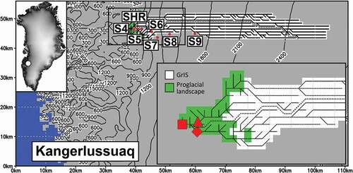
Figure 1. Kangerlussuaq simulation domain and catchment (12,825 km²; GrIS covered part 12,000 km²) with HydroFlow estimated drainage network and watershed divide between Sandflugtsdalen and Ørkendalen (dotted lines), 300-m contour interval, and locations for the K-transect AWSs S4–S9 and SHR (red dots). The inset figure (upper left) indicates the general location in Greenland. The inset figure (lower right) indicates a detailed illustration of the drainage system in the lower part of the catchment (below ~1,500 m a.s.l.), including the location of the Kangerlussuaq catchment outlet at the Watson River bridges (red square), outlet of Sandflugtsdalen (red triangle), and outlet from Ørkendalen (red diamond)

Hasholt et al. (2013) and Mikkelsen et al. (2013, 2016) reanalyzed the observed seasonal runoff conditions at the catchment outlet and the occurrence of jökulhlaups. A new cycle of jökulhlaups from an ice-marginal lake was initiated in 2007 (Russell et al. 2011); the drainage occurred toward the end of the ablation season for all years between 2007 and 2013, except for 2009 and 2011. Further, the runoff peak on July 11, 2012, which followed an extreme GrIS melt extent, was analyzed by Nghiem et al. (2012), Hall et al. (2013), and Hanna et al. (2014). Smith et al. (2015) used satellite mapping and in situ measurements to characterize GrIS supraglacial water storage, drainage patterns, and discharge, whereas Rennermalm et al. (2012, 2013) studied near-margin proglacial river stage, discharge, and water temperature, together with meltwater retention and delay. Recently, van As et al. (2017) updated and strengthened the observed Watson River discharge hydrograph time series (2006–2015) based on new available acoustic doppler current profiler (ADCP) measured discharge. Prior to the study by van As et al. (2017), observed and simulated discharge studies based on model calibration by observed discharge had higher uncertainty and were biased toward an underestimation of discharge. This uncertainty was because of difficulties in measuring the river cross-section profile (bed level variabilities in response to changes in sand deposition and erosion throughout the runoff season), difficulties in measuring the stage level because of the hydraulic jumps, and difficulties in measuring velocity at supercritical conditions (Froude number >1). A revision of the observed Watson River discharge time series was needed, for example, to improve our quantitative understanding of runoff and related transport of sediment and solutes from the Kangerlussuaq catchment, including the delay, onset/end, duration, variation, and intensity of freshwater supply to the fjord Kangerlussuaq. For instance, information about runoff, sediment, and solute transport is needed as boundary conditions in hydrodynamic and ecological fjord models.

Modeling the GrIS surface water balance components, including SMB, is relatively well understood and documented in several studies (e.g., Cullather et al. 2016; Ettema et al. 2009; Fettweis et al. 2013; Hanna et al. 2008; Langen et al. 2015; Mernild et al. 2011; Vernon et al. 2013). The physical mechanisms that connect climate and nonlinearities in meltwater retention and firn densification, feedbacks between hydrology and ice sheet dynamics, and internal runoff routing and storage, which all contribute toward transforming the various input contributions into a runoff hydrograph at the margin, while taking into account the seasonal flow changes and delays, are only weakly understood (e.g., Rennermalm et al. 2013). In spite of this, there is growing recognition that accurate representations of meltwater retention, internal drainage and storage, and flow processes are essential for realistically assessing the impact of climate variability on the GrIS hydrological conditions, including freshwater river runoff (Langen et al. 2016; van As, Box, and Fausto 2016, 2017).

In this study, SnowModel and HydroFlow (Liston and Mernild 2012) were used to simulate climatic and hydrological conditions within the Kangerlussuaq catchment and along the drainage network through the glacierized and non-glacierized parts of the catchment. These simulations focus on the spatiotemporal distribution of energy and moisture fluxes and variabilities. Also, the ratios between river runoff and rain-derived runoff, snowmelt-derived runoff, and glacier ice melt–derived runoff were simulated for the outlet of Watson River together with the river runoff ratio between the tributaries from the two main sub-basins Sandflugtsdalen (in Greenlandic: Akuliarusiarsuup Kuaa) and Ørkendalen (Qinnquata Kuussua; Figure 1). This is to evaluate the importance of rain-derived, snow-derived, and glacier ice–derived runoff, and the spatiotemporal distribution of runoff within the Kangerlussuaq catchment. ERA-I atmospheric data at six-hour temporal resolution (precipitation twelve-hour temporal resolution) were downscaled to three hourly, 5-km, gridded data sets using the MicroMet (Liston and Elder 2006a) meteorological downscaling algorithms and submodels: ERA-I was chosen because it well represented atmospheric and GrIS conditions (Cullather et al. 2016), and because Langen et al. (2015) showed promising results after a full evaluation estimating changes in ice sheet surface mass-balance for the drainage basin linked to the Godthåbsfjord (64° N) in southwest Greenland. These atmospheric forcing data were used to drive SnowModel over the entire GrIS. Direct independently observed GrIS point MAAT and SMB, and catchment-integrated river runoff time series, which partly covered the period 1990–2014, were used to verify the performance of the SnowModel and HydroFlow simulations.

We simulated and analyzed the sub-daily, daily, monthly, annual, and decadal climatic and hydrological conditions covering the period from September 1979 to August 2014 for the Kangerlussuaq catchment. This study focuses on the following research questions: (1) Does simulated GrIS Kangerlussuaq air temperature, SMB, and river runoff agree with observed conditions and trends, including seasonal variabilities? (2) Have trends in GrIS Kangerlussuaq climatic and hydrological conditions been significant since 1979? (3) What is the spatiotemporal distribution of climatic and hydrological conditions within the GrIS Kangerlussuaq catchment? (4) Can we quantify the links between catchment outlet river runoff and contributions from rain-derived runoff, snowmelt-derived runoff, and glacier ice melt–derived runoff? and (5) What is the systematic seasonal distribution (ratio) between river runoff from the tributaries draining the two sub-basins Sandflugtsdalen and Ørkendalen? This study provides us with an extended understanding and update of the climatic and hydrological conditions and trends within the Kangerlussuaq catchment, including an update on the origin of river runoff and spatiotemporal runoff variability within the catchment during the thirty-five-year period (1979–2014).

Model description, setup, and verification

SnowModel

The model simulations were performed using SnowModel (Liston and Elder 2006a) to quantify GrIS spatial and temporal variations in first-order atmospheric forcing, surface snow properties, SMB, and runoff conditions for the Kangerlussuaq catchment (Figure 1). SnowModel downscales and simulates meteorological conditions, calculates a full surface energy balance (considering the influence of cloud cover, sun angle, topographic slope, and aspect on incoming solar radiation), and accounts for moisture exchanges within the simulation domain. The moisture exchange protocols include multilayer heat- and mass-transfer processes within the snow and drainage system and catchment runoff simulations based on a flow network calculated in HydroFlow from gridded surface topography and ocean-mask data (Liston and Mernild 2012). The simulations were conducted using five of the six submodels implemented in SnowModel: MicroMet (Liston and Elder 2006b); Enbal (Liston et al. 1999); SnowTran-3D (Liston et al. 2007; Liston and Sturm 1998); SnowPack-ML (Liston and Mernild 2012); and HydroFlow (Liston and Mernild 2012). For further details about SnowModel and HydroFlow, see Liston and Elder (2006a) and Liston and Mernild (2012).

SnowModel has been developed during the past three decades and tested step-wise with success on snow- and ice-covered land and ice applications: these include the Antarctic ice sheet, the GrIS, and mountain glaciers in the northern hemisphere (specifically Greenland) and southern hemisphere (e.g., Beamer et al. 2016; Hiemstra, Liston, and Reiners 2002, 2006; Liston and Hiemstra 2011; Suzuki et al. 2011; Suzuki, Liston, and Kodama 2015).

These SnowModel studies have all been tested against independent observations and have yielded acceptable results. In addition, the spatiotemporal snow surface albedo routines in SnowModel (Mernild et al. 2010) have been found to realistically evolve individual grid scale snow albedo using the methods of Douville, Royer, and Mahfouf (1995) and Strack, Liston, and Pielke (2004), where the snow albedo gradually decreased from 0.8 to 0.5 as the snow aged. In the present application, the snow albedo was reset to 0.8 after a 0.003 mm snow-water equivalent of newly fallen snow. The albedo for bare ice was set to 0.4 in SnowModel. Alternatively, for example, van As et al. (2017) prescribed the GrIS Kangerlussuaq catchment albedo using Moderate Resolution Imaging Spectroradiometer (MODIS) Terra MOD10A1 data averaged over 100-m elevation bins, but this approach limits studies to the 2000–present temporal extent of MODIS products.

Model configuration and meteorological forcing

The GrIS Kangerlussuaq surface simulations were conducted for the thirty-five-year period from 1979/1980 to 2013/2014, following the “mass-balance year” from September 1 to August 31. The domain covered the GrIS, Greenland coastal regions, and its surrounding fjords and seas (Figure 1). Atmospheric forcings were provided by the ERA-I reanalysis. ERA-I is a global atmospheric reanalysis from 1979, continuously updated in near real time. The ERA-I products are available on a 1° longitude × 1° latitude grid from the European Centre for Medium-Range Weather Forecasts (ECMWF; Dee et al. 2011) and on a six-hour time step. Precipitation, however, was available on a twelve-hour time step. We used the standard (total = large-scale plus convective) precipitation from ECMWF ERA-I reanalysis.

The ERA-I products were aggregated to three hourly values by linear interpolation to resolve the diurnal cycle. The ERA-I forcings were downscaled in MicroMet to create spatiotemporal-distributed atmospheric fields, using the Barnes objective analysis scheme (Barnes 1964, 1973) and known temperature-elevation, wind-topography, humidity-cloudiness, and radiation-cloud-topography relationships (for detailed information, see Liston and Elder 2006a). Depending on the variable of interest, the SnowModel outputs were either summed or averaged to daily, monthly, annual, and/or decadal values.

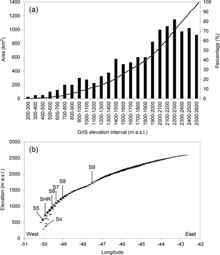
The surface topography data were obtained from Levinsen et al. (2015), and rescaled to a 5-km horizontal grid increment. This digital elevation model (DEM) was a time-invariant DEM specific to the year 2010 (Figure 1). The DEM was developed by merging contemporary radar and laser altimetry data. Radar data were acquired with Envisat and CryoSat-2, and laser data with the Ice, Cloud, and Land Elevation Satellite, Airborne Topographic Mapper, and Land, Vegetation, and Ice Sensor. Radar data were corrected for horizontal, slope-induced errors and vertical errors from penetration of the echoes into the subsurface (Levinsen et al. 2015). Because laser data are not subject to such errors, merging radar and laser data yields a DEM that is capable of resolving both surface depressions and topographic features at higher altitudes (Levinsen et al. 2015). The Kangerlussuaq catchment was estimated to be 12,825 km², with the GrIS covering approximately 12,000 km² of the catchment, indicating that the proglacial tundra area accounts for approximately 6 percent of the entire catchment. Our analysis shows that approximately 50 percent of the Kangerlussuaq GrIS catchment is located below 2,000 m a.s.l. (Figure 2A).

Figure 2. Kangerlussuaq GrIS catchment: (a) hypsometry, and (b) longitudinal elevation profile based on individual grids from the GrIS margin (west) to the highest elevated part of GrIS at the ice sheet divide (east). The locations of the K-transect stakes S4–S9 and SHR are shown

Our HydroFlow-estimated Kangerlussuaq catchment area is larger than that reported in some earlier studies, such as 6,130 km² by Mernild et al. (2011), and 9,743 km² by Hasholt et al. (2013). The difference in catchment area between this study and Mernild et al. (2011) is mainly because of the use of a relatively less accurate DEM (Bamber, Ekholm, and Krabill 2001) and the program RiverTools (http://rivix.com/) for estimating, for example, the watershed divides. Using a detailed bedrock map, Lindbäck et al. (2015) calculated the hydropotential for the region and also found the Kangerlussuaq sector of the GrIS to be approximately 12,000 km², equal to 0.7 percent of the total GrIS area (van As et al. 2017).

The flow residence times and flow velocities of meltwater and rain passing through the HydroFlow grid cells depend on the travel distance (i.e., the grid cell size); surface slope and roughness (e.g., density of depression storage, such as superglacial lakes, crevasses, and moulins); characteristics of the snow and ice matrix that the fluid is flowing through and over (e.g., temperature or cold content and porosity); temporal evolution of the snow and ice matrix; and changes in superglacial, englacial, and subglacial channel dimensions (Liston and Mernild 2012). In HydroFlow, we used flow velocities gained from tracer experiments conducted through the snowpack (in both early and late summer) and through the en- and subglacial environments (Mernild, Hasholt, and Liston 2006). Here, for example, the spatiotemporal variability in simulated snow distribution and associated characteristics have an impact on the transit time and its spatial and temporal evolution through the snowpack (for additional details see Liston and Mernild 2012).

Because of the use of a 5-km horizontal grid increment, snow transport and blowing-snow sublimation processes generated by SnowTran-3D were excluded from the simulations (static sublimation was, however, included in the model integrations) because blowing snow does not typically move completely across 5-km distances. On the GrIS, wind-transported snow particles are typically captured in a drift trap, or they sublimate before traveling several kilometers (Liston and Hiemstra 2011). By not including snow transport and blowing-snow sublimation in these GrIS Kangerlussuaq simulations, the results may underestimate the total annual sublimation, and subsequently influence calculated snowpack properties such as, for example, snow density, snow-water equivalent depths, and snow-cover evolution. Experiences from observational snow studies (Liston and Hiemstra 2011; Sturm et al. 2010) indicate that by excluding snow transport and blowing-snow sublimation processes, we expect simulated snow densities to be approximately 50 kg m⁻³ lower than observations depending on the season of the year. Here we have assumed that the lower-density simulations have not had an impact on processes that move liquid water through the snowpack. Also, surface albedo may be influenced by excluding blowing-snow transport from the simulations, likely slightly underestimating (overestimating) the snow covered (ice covered) areas.

Verification of simulations

Three independent observational data sets were used for MAAT (point observations), SMB (point observations), and catchment freshwater river runoff model verification (Tables 1–3), where river runoff integrates a response of the watershed to precipitation, snow and glacier melt, groundwater flow, and other hydrometeorological processes (e.g., Bliss, Hock, and Radic 2014; Liston and Mernild 2012). For the GrIS at the K-transect (Figure 1), long-term automatic weather station (AWS) MAAT and annual SMB time series have been observed continuously since 1993 and 1990, respectively (e.g., van den Broeke et al. 2008a, 2008b; van de Wal et al. 2005). Data from AWS and stakes for S4–S9 and SHR were used, covering the elevation range from approximately 390 to 1,460 m a.s.l. (Figure 2B). Observed time series of catchment freshwater river runoff for Greenland and the GrIS are sparse; available runoff data sets represent less than 1 percent of the total Greenland runoff that is transferred to the surrounding fjords and seas (Mernild and Liston 2012). However, at the Kangerlussuaq catchment, river runoff has been observed at the Watson River since 2006 (e.g., Mernild and Hasholt 2009; Mernild et al. 2011; Hasholt et al. 2013; Mikkelsen et al. 2013; van As et al. 2012, 2017; Figure 1). These runoff time series have been adjusted and recalculated several times to account for: (1) a wider range of observed discharges that could be used to strengthen the stage discharge relation; (2) new soundings of the river cross-section profile, including the bottom profile, to better understand the bed-level variability in response to changes in sand deposition and erosion throughout the runoff season; and (3) recognition of uncertainty of the determination of surface level and velocity under supercritical hydraulic conditions, including the presence of hydraulic jumps. The river discharge time series—updated using ADCP measurements by van As et al. (2017)—are twice as large as values by Hasholt et al. (2013) and four times as large as those observed by Mernild and Hasholt (2009; for a detailed description of the updated Watson River time series, including uncertainties, see van As et al. [2017]). These updated observed runoff time series impact earlier simulations of runoff (e.g., Mernild et al. 2011, 2012), because these simulations were verified against underestimated river discharge. The observed runoff time series cover the runoff season, except before mid-May and after late-September when there is risk of frost damage to the stage instruments (van As et al. 2017).

Table 1. Observed and SnowModel ERA-I simulated MAAT and standard deviation for the different K-transect AWS S5, S6, and S9 for variable observation periods and 1979–2014. Observed data from the AWS are operated by IMAU (van de Wal et al. 2005)

	S5	S6	S9
Observed (°C), period	−6.3 ± 8.2 (August 1993–August 2014)	−9.9 ± 8.3 (August 1995–August 2014)	−12.7 ± 8.6 (August 2003–August 2014)
Simulated (°C), period	−6.1 ± 9.3 (August 1993–August 2014)	−9.5 ± 8.5 (August 1995–August 2014)	−12.2 ± 8.2 (August 2003–August 2014)
Simulated (°C), 1979–2014	−6.7 ± 9.4	−9.4 ± 8.9	−12.3 ± 8.3

Table 2. Observed and SnowModel ERA-I simulated SMB mean and standard deviation for the different K-transect stakes S4–S9 and SHR for two periods 1990–2014 and 1979–2014. The value in the brackets illustrates the mean difference between observed and simulated SMB

	S4	S5	SHR	S6	S7	S8	S9	Mean
Observed 1990–2014 (m w.e yr^−1)	−4.15 ± 0.71	−3.68 ± 0.64	−3.08 ± 0.59	−1.66 ± 0.57	−1.48 ± 0.60	−0.78 ± 0.59	−0.12 ± 0.41	−2.14 ± 0.59
Simulated 1990–2014(m w.e yr^−1)	−3.83 ± 0.57	−3.56 ± 0.60	−3.21 ± 0.64	−2.24 ± 0.68	−1.94 ± 0.69	−1.08 ± 0.66	−0.32 ± 0.58	−2.31 ± 0.63 (0.17 ± 0.23)
Simulated 1979–2014(m w.e yr^−1)	−3.70 ± 0.56	−3.43 ± 0.58	−3.09 ± 0.62	−2.11 ± 0.66	−1.82 ± 0.67	−0.94 ± 0.65	−0.19 ± 0.55	−2.18 ± 0.61

Table 3. Observed and SnowModel ERA-I simulated mean Watson River outlet runoff and standard deviation for the years 2007–2013. Observed runoff is operated by GEUS (van As et al. 2012, 2017)

	2007	2008	2009	2010	2011	2012	2013	Mean
Observed discharge (m^3) (observed period)	7.51 × 10^9 (June 7–September 8)	5.46 × 10^9 (May 27–September 10)	4.87 × 10^9 (June 2–September 9)	11.24 × 10^9 (May 10–September 28)	7.77 × 10^9 (June 7–September 18)	10.73 × 10^9 (May 28–September 30)	4.32 × 10^9 (June 6–September 15)	7.41 × 10^9
Simulated discharge (m^3) (observed period)	11.65 × 10^9 (June 7–September 8) (63%)	8.04 × 10^9 (May 27–September 10) (66%)	6.67 × 10^9 (June 2–September 9) (69%)	13.66 × 10^9 (May 10–September 28) (82%)	11.68 × 10^9 (June 7–September 18) (66%)	14.97 × 10^9 (May 28–September 30) (71%)	8.22 × 10^9 (June 6–September 15) (52%)	10.69 × 10^9 (68 ± 9%)
Simulated discharge (m^3) (entire runoff period)	12.12 × 10^9	8.72 × 10^9	7.11 × 10^9	14.14 × 10^9	12.85 × 10^9	15.36 × 10^9	8.57 × 10^9	11.26 × 10^9
Adjusted simulated discharge (m^3) (entire runoff period)	7.67 × 10^9	5.75 × 10^9	4.89 × 10^9	11.53 × 10^9	8.54 × 10^9	10.94 × 10^9	4.45 × 10^9	7.69 × 10^9

These independent catchment observations (point MAAT, point SMB, and catchment outlet river runoff) were used for verification of SnowModel/HydroFlow simulations, even though these available data sets do not cover the complete simulated spatial and temporal domains. However, they remain useful for verification of SnowModel/HydroFlow ERA-I simulated GrIS MAAT, SMB, and catchment river runoff conditions (Tables 1–3).

In the presentation that follows, all comparisons and correlation trends that are declared significant are statistically significant at or above the 5percent level (p < 0.05; based on a linear regression t test, where p equals the level of significance).

Water balance components

For the Kangerlussuaq catchment and for the GrIS surface water balance components, the following Equation 1(1) $P-(Su+E)-R+\mathrm{\Delta }S=0\pm \eta ,$(1) can be estimated in SnowModel based on the hydrological method (continuity equation):

(1) $P-(Su+E)-R+\mathrm{\Delta }S=0\pm \eta ,$(1)

where P is precipitation input from snow and rain; Su is sublimation (solid to gas phase with no intermediate liquid stage) from a static surface; E is evaporation (liquid to gas phase flux of water); R is runoff from snowmelt, ice melt, and rain; ΔS is change in storage (ΔS is also referred to as SMB) derived as the residual value from changes in glacier storage and snowpack storage. For snow and ice surfaces, the ablation was estimated as: Su + E + R. The parameter η is the water-balance discrepancy (error). The error term should be 0 (or small), if the components P, Su, E, R, and ΔS have been determined accurately.

Results and discussion

Verification of MAAT, SMB, and runoff simulations

Table 1 shows point-observed and grid-simulated MAAT for the K-transect for AWS S5, S6, and S9. For all three AWS, simulated MAAT is not significantly different from observed MAAT with mean differences of 0.2°C (S5; August 1993–August 2014), 0.4°C (S6; August 1995–August 2014), and 0.5°C (S9; August 2003–August 2014). This provides confidence in SnowModel ERA-I simulated GrIS MAAT, although the difference between the simulated and observed MAAT increases with increasing elevation (Table 1).

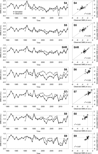
Regarding verification between point-observed and grid-simulated annual SMB time series (1990–2014) for the K-transect for AWS, S4–S9 and SHR showed small mean differences between time series (Table 2): For each individual AWS, the mean annual difference between point-observed SMB and grid-simulated SMB span between minimum 0.12 m w.e. (S5) and maximum 0.58 m w.e. (S6), averaging 0.17 ± 0.23 m w.e. (where ± is standard deviation). This indicates confidence in SnowModel ERA-I simulated annual SMB along the K-transect (Table 2). Further, Figure 3 shows annual time series and scatter plots of observed (point) and simulated SMB (grid), highlighting r² values (where r² is the explained variance) in the range between 0.55 and 0.67 (linear), except for AWS S6 (elevation ~1,000 m a.s.l.), where r² was 0.28 and the simulated SMB was slightly lower than the observed SMB after 1995. The simulated thirty-five-year mean equilibrium-line altitude (ELA; the spatially averaged elevation of the equilibrium line, defined as the set of points on the glacier surface where the net mass balance is zero) was located at 1,760 ± 260 m a.s.l. van As et al. (2017) estimated ELA, here defined as the altitude where SMB minus refreezing equals zero, to be at approximately 1,800 m a.s.l. (2009–2015), and van de Wal et al. (2012) at approximately 1,610 m a.s.l. (1991–2014).

Figure 3. SnowModel ERA-I simulated (1979–2014) and observed (1990–2014) SMB time series and scatter plots for the different K-transect stakes S4–S9 and SHR

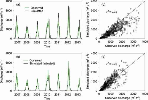
Catchment outlet runoff is an integrated response of all hydrometeorological processes within the catchment, including GrIS supra-, en-, and subglacial processes. Daily simulated catchment outlet discharge hydrograph time series (Watson River) were verified against observed discharge hydrograph time series (not including early- and late-season discharge values; Figure 4). Simulated discharge values followed observed discharge values related to the time for initiation/ending of seasonal runoff and the time and size of daily peak discharges. For example, for July 11–14, 2012 (during the period of extreme GrIS surface melt; Hanna et al. 2014; Nghiem et al. 2012), the mean daily observed discharge averaged approximately 2,980 m³ s⁻¹ and the simulated runoff was approximately 3,150 m³ s⁻¹, indicating an overestimation of about 5 percent (Figure 4A). Besides the scatter plot illustrated on Figure 4B between daily observed and simulated discharge (r² = 0.72, linear), we performed a Nash–Sutcliffe coefficient (NSC) test (Nash and Sutcliffe 1970), which showed a NSC value of 0.54. If the NSC is 1, then the model is a perfect fit to the observations. If the NSC is between 1 and 0, decreasing values represent a decline in goodness of fit, where zero and negative values represent major deviations between the modeled and observed data.

Figure 4. Kangerlussuaq catchment observed and SnowModel ERA-I simulated daily discharge (2007–2013): (a) time series, (b) scatter plot, (c) adjusted discharge time series, and (d) adjusted discharge scatter plot

In Table 3, simulated runoff has for each individual year been compared against observed runoff (for the exact same time period). This comparison shows an overestimation of simulated runoff of 31 ± 9 percent (2007–2013). This overestimation of outlet runoff is not the result of significant differences between simulated and observed GrIS air temperature and SMB conditions (Tables 1 and 2), but is likely because of model uncertainties; for example, not representing the proper catchment delineations and area (Lindbäck et al. 2015) and/or spatiotemporal processes related to multiyear meltwater retention, percolation (blocked by ice layers), and refreezing processes and routines in multiyear firn layers on the ice sheet. Such snow and firn processes have an influence on percolation and runoff flow conditions (Langen et al. 2016), as surface melt does not necessarily equal runoff because meltwater can refreeze in the porous near-surface snow and firn, making the firn layer an important buffer (Janssens and Huybrechts 2000; Machguth et al. 2016).

Harper et al. (2012) emphasized that surface melt generated in the percolation zone (a region of the accumulation area that is perennially covered by snow and firn) is poorly constrained, where a proportion of meltwater will infiltrate the snow, firn, and multi-firn layer, and a proportion will flow downstream to lower GrIS elevations. Understanding the multiannual spatiotemporal meltwater percolation, retention, and refreezing processes and routines in the snow and the multiyear firn layers is still far from solved (van As, Box, and Fausto 2016). However, SnowModel/HydroFlow is one of the few GrIS SMB models, apart from, for example, Lewis and Smith (2009) and Lindbäck et al. (2015), that is able to route meltwater in a spatial gridded system.

In SnowModel/HydroFlow, the flow network is controlled exclusively by surface topography, whereas the role of bedrock topography on controlling the potentiometric surface and the associated flow direction is secondary (Cuffey and Paterson 2010) from the flow’s place of origin to the ice sheet margin and to the coastline. Simulated runoff volumes were therefore adjusted to match observed runoff volumes, showing that the mean annual adjusted runoff was 7.7 ± 10⁹ m³ yr⁻¹ (2007–2013), spanning from 4.9 ± 10⁹ m³ yr⁻¹ (2009) to 11.5 ± 10⁹ m³ yr⁻¹ (2010). In comparison, the observed mean annual runoff was 7.41 ± 10⁹ m³ yr⁻¹ (Table 3), which is within the range of acceptance. A linear relation between daily observed and simulated adjusted runoff indicates a r² value of 0.76, and an NSC value of 0.75. The simulated adjusted runoff follows observed runoff values related to the time for initiation/ending of seasonal runoff and time and amount of peak discharges. For example, for July 11–14, 2012, the mean daily observed discharge was on average approximately 2,980 m³ s⁻¹, and simulated adjusted runoff was approximately 2,710 m³ s⁻¹ (Figure 4C), indicating an underestimation of 9 percent (henceforth, adjusted runoff is referred to as runoff).

Seasonal and annual variabilities in GrIS Kangerlussuaq surface conditions

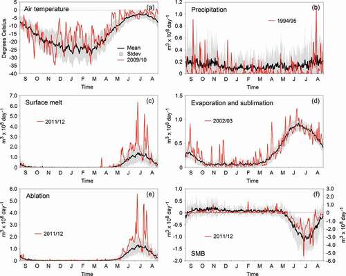
Figure 5 emphasizes the thirty-five-year mean seasonal variability in GrIS Kangerlussuaq surface parameters. GrIS-average air temperature conditions show a characteristic variability—a distinct annual cycle—with thirty-five-year mean minimum temperatures through winter of approximately −25°C (December through February) and maximum temperatures through summer of approximately −5°C (June through August; Figure 5A). Precipitation was lowest during December through March (~0.1 × 10⁸ m³ d⁻¹) and highest during the period August–November (~0.2 × 10⁸ m³ d⁻¹; Figure 5B). This variability is confirmed by precipitation observations (operated by DMI; Mernild et al. 2015), although it must be emphasized that these data were observed in the town of Kangerlussuaq (~30 km west of the ice sheet margin). Surface melt occurred from May through September, with the highest thirty-five-year mean values throughout July (~1.2 × 10⁸ m³ d⁻¹; Figure 5C), following the seasonal pattern from, for example, Tedesco et al. (2014). As expected, evaporation, sublimation, and ablation had similar seasonal thirty-five-year mean patterns as surface melt (Figure 5D, E), where, for example, the seasonal variability in evaporation and sublimation follows values from Boisvert et al. (2016). The thirty-five-year mean SMB seasonal variability indicates positive SMB from September through May, followed by negative SMB with the most negative values in July (~1.0 × 10⁸ m³ d⁻¹; Figure 5F). The GrIS Kangerlussuaq SMB pattern follows the overall seasonal ice sheet SMB variability as shown, for example, on the online Polar Portal (http://polarportal.dk/en/groenlands-indlandsis/nbsp/isens-overflade/). With respect to GrIS Kangerlussuaq surface melt, ablation, and SMB, 2011/2012 was an extreme year within the thirty-five-year period (Figure 5C, E, F); this is also confirmed by observations by Nghiem et al. (2012) and van As et al. (2017).

Figure 5. Kangerlussuaq GrIS catchment thirty-five-year mean daily SnowModel ERA-I simulated surface (1979–2014): (a) air temperature, (b) precipitation, (c) surface melt (snow and ice melt), (d) evaporation and sublimation, (e) ablation, and (f) SMB. The bold black line is the daily mean, the grey area indicates one standard deviation, and the red line indicates the year with the maximum accumulated value (for precipitation and SMB it is the yearly minimum accumulated values)

In Figure 6, the annual time series of GrIS Kangerlussuaq surface parameters (1979–2014) are shown together with linear trends (only significant trends are shown). For the GrIS Kangerlussuaq catchment, MAAT was −15.0 ± 1.4°C, precipitation was 0.42 ± 0.08 m w.e. yr⁻¹, surface melt was 0.81 ± 0.26 m w.e. yr⁻¹, evaporation and sublimation were 0.10 ± 0.01 m w.e. yr⁻¹, ablation was 0.76 ± 0.23 m w.e. yr⁻¹, and SMB was −0.34 ± 0.24 m w.e. yr⁻¹. For the ERA-I grid point located closest to the center of the Kangerlussuaq watershed, MAAT was −15.2 ± 1.5°C and precipitation was 0.43 ± 0.09 m w.e. yr⁻¹ (the ERA-I grid point annual time series are shown in red on Figure 6). MAAT, surface melt, ablation, and SMB displayed significant trends (Figure 6A–F). SMB was the only parameter with a negative trend. For SMB, it was close to zero in 1980, dropping to approximately −0.6 m w.e. yr⁻¹ in 2014 (−0.14 m w.e. decade⁻¹; linear). MAAT, surface melt, and ablation changed on average from approximately −16°C to −14°C (0.78°C decade⁻¹), approximately 0.4 to 1.1 m w.e. yr⁻¹ (0.17 m w.e. decade⁻¹), and approximately 0.5 to 1.0 m w.e. yr⁻¹ (0.14 m w.e. decade⁻¹), respectively (Figure 6). Similar trends have previously been shown, for example, for Godthåbsfjorden (Langen et al. 2015), and for the entire GrIS (Hanna et al. 2011; Tedesco et al. 2014; Fettweis et al. 2008, 2011, 2016; Wilton et al. 2017).

Figure 6. SnowModel ERA-I simulated time series of Kangerlussuaq GrIS catchment: (a) MAAT, (b) precipitation, (c) surface melt (snow and ice melt), (d) evaporation and sublimation, (e) ablation, and (f) SMB. Only significant trends are shown as linear fits through the data. For both (a) MAAT and (b) precipitation, ERA-I data are shown for the grid point located closest to the center of the Kangerlussuaq catchment (red time series). The grey shading is the ±10 percent (forced by a change in precipitation of ±10%). It is most visual for precipitation and SMB

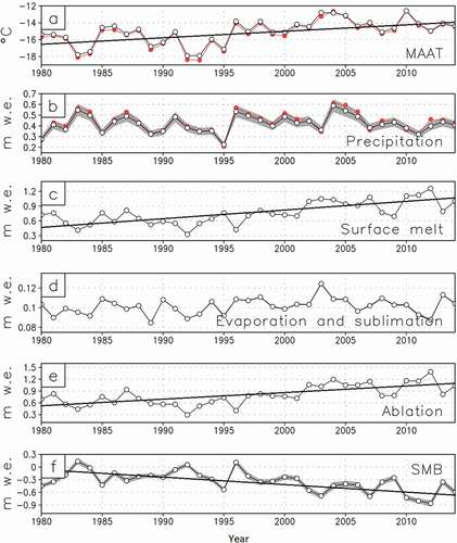
An uncertainty analysis can be conducted by applying a positive and negative 10 percent precipitation bias to the SnowModel ERA-I simulations (grey shading on Figure 6). The results of this test showed that the mean annual catchment SnowModel ERA-I precipitation was insignificantly different with respect to potentially biased values: 0.42 ± 0.08 m w.e. yr⁻¹ (precipitation), 0.46 ± 0.09 m w.e. yr⁻¹ (precipitation +10%), and 0.38 ± 0.07 m w.e. yr⁻¹ (precipitation −10%). A similar effect occurred for SMB where the difference also was insignificant: −0.34 ± 0.24 m w.e. yr⁻¹ (SMB), −0.28 ± 0.24 m w.e. yr⁻¹ (SMB simulated based on +10% precipitation), and −0.40 ± 0.24 m w.e. yr⁻¹ (SMB simulated based on −10% precipitation). We therefore conclude that less impact was seen on SMB by applying a positive and negative 10 percent precipitation bias to the simulations.

Spatial variability in GrIS Kangerlussuaq surface conditions

For the GrIS Kangerlussuaq catchment, the relationship between MAAT distribution and elevation showed that the thirty-five-year MAAT was, as expected, highest at the ice sheet margin (~ −5°C) and lowest at highest elevations near the ice divide (~ −21°C; Figures 7A and 8A). The thirty-five-year mean 0°C isotherm was located at elevations near the ice sheet margin (<280 m a.s.l.). In addition to MAAT, precipitation is a key climate system variable. Figures 7B and 8B show the thirty-five-year mean precipitation versus elevation, including the fraction of annual precipitation falling as snow and rain, where snow precipitation accounted for 95 percent (0.40 ± 0.08 m w.e. yr⁻¹) of the total mean annual precipitation (Figure 7B)—this indicates that the GrIS Kangerlussuaq catchment is influenced by a snow-dominated precipitation regime. In Figures 7B and 8B, the thirty-five-year mean precipitation versus elevation show an increasing precipitation (significant) with increasing elevation (~0.1 m w.e. 100 m⁻¹), with lowest mean annual values at the GrIS margin (~0.25 m w.e. yr⁻¹) and highest values at the ice sheet divide (~0.54 m w.e. yr⁻¹). However, at elevations between approximately 1,800 and 2,400 m a.s.l., there is a drop in precipitation from about 0.45 m w.e. to 0.40 m w.e., controlled by variabilities in snow precipitation (Figures 7B and 8B). This indicates, above approximately 1,800 m a.s.l., a C-shaped precipitation distribution pattern with increasing elevation. Overall, this suggests considerable spatial variability in precipitation with increasing elevation within the GrIS catchment over distances of a few tens of kilometers (Figures 7B and 8B). The amount of snow precipitation increased with increasing elevation (significant; except between ~1,800 and ~2,400 m a.s.l.). The amount of rain decreased with increasing elevation (significant; Figure 7B) because of the decreasing trend in MAAT (Figure 7A). The annual amount of snowfall relative to the total amount of precipitation was 45 percent at the ice sheet margin (~280 m a.s.l.), 75 percent (~1,000 m a.s.l.), 90 percent (~1,500 m a.s.l.), and 98 percent (~2,000 m a.s.l.; Figure 7B).

Figure 7. SnowModel ERA-I simulated thirty-five-year: (a) MAAT, (b) precipitation (snow and rain), (c) surface melt (snow and ice melt), (d) evaporation and sublimation, (e) ablation, and (f) SMB versus elevation

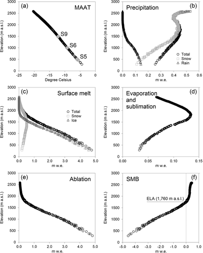
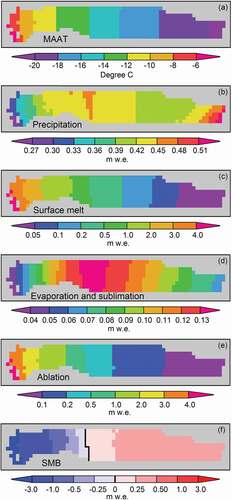
Figure 8. SnowModel ERA-I simulated thirty-five-year mean spatial Kangerlussuaq GrIS catchment surface (1979–2014): (a) MAAT, (b) precipitation, (c) surface melt (snow and ice melt), (d) evaporation and sublimation, (e) ablation, and (f) SMB

Figures 7C and 8C show the thirty-five-year mean surface melt versus elevation for the GrIS Kangerlussuaq catchment, indicating decreasing melt with increasing elevation, as expected. Ice melt follows the overall trend in surface melt, where at less than 1,500 m a.s.l. the amount of ice melt is greater than snowmelt (0.6 m w.e.), and opposite at greater than 1,500 m a.s.l. (Figure 7C). Furthermore, snowmelt was greatest at approximately 1,500 m a.s.l. (0.6 m w.e.) because of a combination of elevation changes in air temperature and precipitation. Evaporation and sublimation peaked at about 1,800 m a.s.l. (0.13 m w.e.), showing similar thirty-five-year mean values of 0.06 m w.e. both at approximately 1,000 and 2,500 m a.s.l. (Figures 7D and 8D). For the GrIS, Boisvert et al. (2016) estimated water fluxes (evaporation and sublimation) to be greatest in the interval between 300 and 1,500 m a.s.l. and lower both below and above this interval. This suggests that the overall GrIS pattern is similar to the regional pattern for the GrIS Kangerlussuaq catchment. In the GrIS Kangerlussuaq catchment, the ablation changed with increasing elevation from approximately 4.8 m w.e. at the ice sheet margin to about 0.05 m w.e. at the ice divide (Figures 7E and 8E). Fausto and van As (2012, updated) estimated annual ablation rates at AWS KAN_L (~670 m a.s.l.; operated by GEUS) to be in the range of 3.2–4.9 m w.e. yr⁻¹ (2009–2014), averaging 3.7 ± 0.8 m w.e. yr⁻¹. Simulated mean ablation ranges at the KAN_L elevation was about 3.8 ± 0.9 m w.e. yr⁻¹ (Figure 7E), with a range of 3.0–4.9 m w.e. (2009–2014). SMB increased with increasing elevation ranging from approximately −4.6 m w.e. yr⁻¹ at the ice sheet margin to about 0.5 m w.e. yr⁻¹ at the ice divide, indicating that the thirty-five-year mean ELA was located at 1,760 m a.s.l. (Figures 7F and 8F). Mean SMB values are in the range of simulated SMB data (1-km resolution; 1958–2015) by Noël et al. (2016).

Runoff from Kangerlussuaq catchment

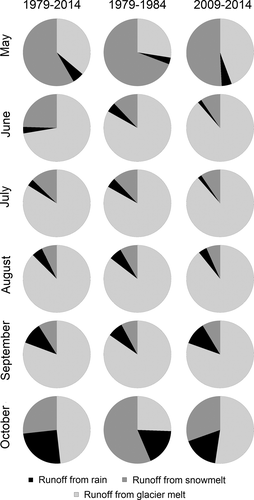
Figure 9A presents the time series of daily simulated discharge (1979–2014) for the Watson River outlet; clearly showing seasonal variability in the hydrograph from no runoff during winter to river runoff during spring, summer, and autumn, and averaging 318 ± 396 m³ d⁻¹ for days with runoff. The runoff time series is tied to runoff contributions from rain-derived runoff, snowmelt-derived runoff, and ice melt–derived runoff. In Figure 9B, the annual variability in runoff contributions from rain-derived runoff, snowmelt-derived runoff, and ice melt–derived runoff is shown, illustrating that the runoff regimes are dominated by ice-melt conditions rather than by a pluvial (rain) or a nival regime. Throughout the study period, between 70 and 90 percent of the annual runoff originated from ice melt–derived runoff (averaging 80 ± 5%), 8–20 percent derived from snowmelt (15 ± 5%), and 2–8 percent derived from rain (5 ± 1%; Figure 9B, C). The catchment runoff was dominated by ice melt–derived runoff due to the glacier cover distribution (~94% of the catchment was covered by the GrIS; according to Lindbäck et al. 2015 it was ~95%), hypsometry, and climate conditions (Figure 1). Also, at the monthly time scale the percentage of runoff contribution from rain-derived runoff, snowmelt-derived runoff, and ice melt–derived runoff is shown in Figure 10. The thirty-five-year mean runoff throughout the runoff season—from May to October—indicated a relative drop in snowmelt-derived runoff from May to August, and hereafter an increase. This shows that snowmelt influences runoff mostly in the beginning of the runoff season (in May). For ice melt–derived runoff, the trend was the opposite, indicating a relative increase from May to August, and a drop hereafter where ice melt influenced the runoff mostly in June through October (Figure 10). Regarding the rain-derived runoff, the relative values were in the same order of magnitude for May through August, hereafter increasing toward the end of the runoff season. Monthly mean runoff variabilities were not significantly different compared to mean values for the first (1979–1984) and last pentad (2009–2014) of the simulation period (Figure 10).

Figure 9. (a) SnowModel ERA-I time series of simulated daily Kangerlussuaq catchment outlet discharge from September 1979 to August 2014; (b) the origin and variability of annual runoff from rain, snowmelt, and ice melt; and (c) thirty-five-year mean runoff contributions (in percentage) from rain, snowmelt, and ice melt

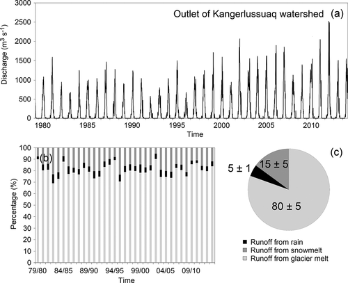
Figure 10. SnowModel ERA-I simulated monthly mean runoff from rain, snowmelt, and ice melt for the runoff season May through October for 1979–2014, 1979–1984, and 2009–2014 for the outlet of Kangerlussuaq watershed

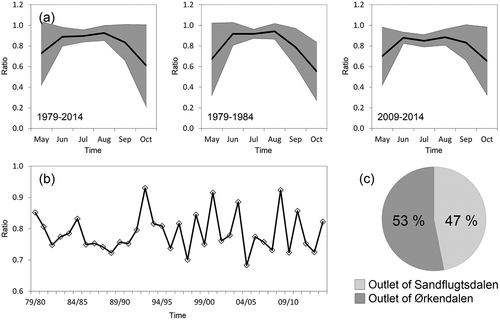
A few kilometers upstream from the Watson River outlet, two tributary rivers from Ørkendalen and Sandflugtsdalen merge (Figure 1). The daily discharge time series from each sub-basin are shown in Figure 11A, B. The mean daily discharge from Ørkendalen was 251 ± 315 m³ s⁻¹ (covering a mean runoff period of 205 d yr⁻¹), whereas the mean daily discharge from Sandflugtsdalen was 238 ± 272 m³ s⁻¹ (191 d yr⁻¹), indicating on average no significant difference in runoff between the two tributaries. On Figure 11C, the daily discharge ratio between Sandflugtsdalen and Ørkendalen indicates variability throughout the runoff season. Such variabilities are highlighted on mean monthly scales for the periods 1979–2014, 1979–1984, and 2009–2014 (Figure 12A), where the ratio in the beginning (May) and the end (October) of the runoff season is close to 0.6–0.7, and between 0.8 and 1.0 for June through September. On an annual time scale, the discharge ratio varies between 0.70 and 0.95 for the thirty-five-year period, averaging 0.79 ± 0.06 (Figure 12B). In other words, at the intersection where the Ørkendalen tributary and the Sandflugtsdalen tributary meet, 53 ± 1 percent of the runoff originated from Ørkendalen sub-basin and 47 ± 1 percent from the Sandflugtsdalen sub-basin during the thirty-five-year period (Figure 12).

Figure 11. SnowModel ERA-I daily simulated discharge September 1979 through August 2014: (a) outlet of Sandflugtsdalen (6,800 km² and GrIS covered part 6,225 km² [92%], illustrated by a red triangle on Figure 1); (b) outlet of Ørkendalen (5,925 km² and GrIS covered part 5,775 km² [97%], illustrated by a red diamond on Figure 1); and (c) ratio between Sandflugtsdalen and Ørkendalen

Figure 12. SnowModel ERA-I simulated: (a) mean monthly runoff ratio between Sandflugtsdalen and Ørkendalen for the annual runoff period (May through October) for 1979–2014, 1979–1984, and 2009–2014, where the gray area equals one standard deviation; (b) time series of mean annual runoff ratio; and (c) the thirty-five-year mean runoff ratio

Model limitations, knowledge gaps, and uncertainty

The SnowModel/HydroFlow simulations over the GrIS Kangerlussuaq catchment show a detailed and physically realistic representation of surface snow and ice ablation, snowpack evolution, SMB, and runoff routing based on the established flow network at relatively high temporal and spatial resolution compared with previous studies by Mernild et al. (2011, 2012). SnowModel/HydroFlow capabilities present a contrast with studies that (1) largely rely on air temperature as a proxy for the energy available for melt, and (2) do not link between surface runoff production from snowmelt and ice-melt processes and the associated freshwater fluxes to downstream areas and surrounding oceans through an estimated flow network that combines the individual grid cells that make up the simulation catchment. HydroFlow takes advantage of its ability to simulate and subsequently display hydrographs at different locations within the drainage network (and at the catchment outlet); for example, at the intersection between the Ørkendalen and Sandflugtsdalen tributaries. In addition, to understand GrIS surface processes, sub-diurnal simulation time steps are required to account for the sub-daily variability in solar radiation and its energy-related surface water balance components, including SMB and runoff. This is because over GrIS ice and snow surfaces, incoming solar radiation is the primary source of energy melting the ice and snow; an order of magnitude greater than that provided by sensible heat flux associated with near-surface air temperatures (Liston and Hiemstra 2011).

However, SnowModel only performs one-way atmospheric coupling in its simulations, where the meteorological conditions are prescribed at each time step. The model simulations were conducted without regard for whether the surface ice and snow distribution and properties might be different from the original ERA-I forcings. In nature the atmospheric conditions would be modified in response to changes in surface conditions and properties (Liston and Hiemstra 2011). Such interactions were unfortunately not accounted for in the Kangerlussuaq SnowModel simulations described herein.

SnowModel used a constant ice sheet area and a time-invariant DEM specific to the year 2010 throughout the simulation campaign (Levinsen et al. 2015). By doing so, the simulations neglect potential SMB feedbacks, for example, from thinning ice and ice retreat and from changes in hypsometry, where changes in hypsometry are expected to be an amplifier of meltwater runoff in a warming climate. Information from satellite observations show that the GrIS margin and hypsometry have changed throughout the past decades (e.g., Kargel et al. 2012). The use of a constant GrIS area and a time-invariant DEM will likely overestimate melt rates, SMB, and runoff prior to 2010, and the opposite will occur after 2010. The overestimation before 2010 is because of a lower elevated GrIS surface compared to reality, and after 2010 the opposite occurred. However, it is not clear whether a change in GrIS margin since 1979 can be resolved with the 5-km grid increment used in these simulations. Further, blowing snow sublimation was not simulated on this 5-km grid. However, the simulations did take into account sublimation over static snow and ice surfaces. Therefore, sublimation might be underestimated (but likely not enough to explain the overestimation in simulated runoff). Static-surface sublimation in SnowModel and in nature depend on the near-surface air temperature, the moisture deficit of the air, wind speed, and components of the surface energy balance (Liston and Hiemstra 2011). Throughout the Arctic, snow studies have shown that the amount of calculated sublimation (blowing and static sublimation) range between 10 and 50 percent of the total winter precipitation (Liston and Sturm 1998, 2004).

Understanding the physical link between a changing climate, snow and ice surface melt, and freshwater river runoff is challenging, and more extensive and accurate records of percolation (blocked by ice layers, likely semipermeable impermeable layers) and refreezing processes and routines in the snow, firn, and the multiyear firn layers on the ice sheet are needed (van As, Box, and Fausto 2016). This is especially true when predicting and modeling nonlinear changes in the permeability of firn and multiyear firn layers. In situ meltwater retention and densification observations in the snowpack, firn pack, and the multiyear firn layers together with impermeable ice layers are physical mechanisms leading to nonlinearity in meltwater retention. Densification, refreezing, and meltwater penetration are difficult processes to observe and quantify in the firn zone (Brown et al. 2012; Humphrey et al. 2012). Hence, present meltwater retention and densification models for each grid assume homogeneous infiltration of percolating meltwater into the firn (e.g., Fettweis et al. 2011). In reality, tracer experiments show chaotic infiltration patterns of both horizontal and vertical water flow established by two flow regimes: “preferential flow” followed by “matrix wetting front flow” (Humphrey et al. 2012). These flow regimes are still not well understood (e.g., Bøggild, Forsberg, and Reeh 2005; van As, Box, and Fausto 2016). The preferential flow system appears in well-defined flow fingers, where the matrix flow system is dominated by film and capillary flow in the unsaturated snow and firn matrix (e.g., Waldner et al. 2004). From a model development perspective, this study shows that SnowModel could be improved by including an extended spatiotemporal and subgrid description of meltwater percolation (e.g., blocked by surface parallel ice layers), refreezing, densification that accounts for nonlinear interactions and feedbacks, and generally a more physical description of the 3-D flow structure in the firn and multiyear firn layers. Such model-development perspectives will strengthen our understanding and better establish the linkages between the GrIS surface hydrological conditions and the hydrographic and circulation conditions in fjords, such as the fjord Kangerlussuaq.

Conclusions

The merging of SnowModel/HydroFlow (a snow, ice, and runoff evolution model) with ERA-I atmospheric forcing data allowed us to simulate, map, and analyze spatiotemporal meteorological, ablation, and freshwater runoff flow conditions for the Kangerlussuaq catchment for the thirty-five-year period 1979–2014, on a three-hour time step and a 5-km grid. SnowModel ERA-I simulated MAAT and SMB were verified against independent observations from the K-transect, indicating an insignificant difference between simulations and observations. Furthermore, simulated freshwater river discharge at the Watson River outlet was verified against observations, initially because of an overestimation of simulated discharge values. Simulated discharge values were overestimated by an average of 31 percent (before verification) compared to observed discharge values, likely because of the lack of model routines; for example, taking into account nonlinearity in meltwater retention and densification in the firn and multiyear firn layers.

In the Kangerlussuaq catchment, the GrIS covered approximately 90 percent of the area, and the thirty-five-year mean GrIS air temperature was −15.0 ± 1.4°C, precipitation 0.42 ± 0.08 m w.e. yr⁻¹, ablation 0.76 ± 0.23 m w.e. yr⁻¹, and SMB −0.34 ± 0.29 m w.e. yr⁻¹. MAAT, surface melt, ablation, and SMB all had significant linear trends over time. The GrIS was influenced by a snow-dominated precipitation regime.

The SnowModel/HydroFlow simulations estimated the flow network within the catchment calculated from the gridded surface topography and ocean-mask data. These HydroFlow river flow simulations expand the possibility to assess the variability in runoff upstream from the catchment outlet; for example, where the two tributary rivers from Ørkendalen and Sandflugtsdalen are merging. On average, 53 percent of the runoff (here illustrated as mean daily discharge: 251 ± 315 m³ s⁻¹) originated from the sub-basin Ørkendalen and 47 percent (238 ± 272 m³ s⁻¹) from Sandflugtsdalen. On average, the difference in runoff from Ørkendalen and Sandflugtsdalen is insignificant; however, it covers a seasonal variability in the runoff ratio between the two sub-basins. At the Watson River outlet a clear variability in the hydrograph occurred, from no winter runoff to seasonal variabilities in discharge during the runoff season, averaging 318 ± 396 m³ d⁻¹, indicating that the runoff regimes are dominated by ice-melt conditions rather than a pluvial (rain) or a nival regime. Throughout the thirty-five-year period, between 70 and 90 percent of the annual runoff originated from ice melt–derived runoff (averaging 80 ± 5%), 8–20 percent derived from snowmelt (15 ± 5%), and 2–8 percent derived from rain (5 ± 1%).

Furthermore, this Kangerlussuaq catchment SnowModel/HydroFlow setup and simulations allow future assessments of the link between the GrIS surface hydrological conditions and the hydrographic and circulation conditions in the adjacent fjords.

Acknowledgments

We extend a special thanks to the two anonymous reviewers for their insightful critique of this article. Observed point air temperature and surface mass-balance data from the K-transect were provided by the Institute for Marine and Atmospheric Research (IMAU), Utrecht University, and Watson River discharge was monitored by B. Hasholt and A.B. Mikkelsen (University of Copenhagen, 2006–2013), and by D. van As and B. Hasholt (Geological Survey of Denmark and Greenland, 2014–present). All SnowModel/HydroFlow data requests should be addressed to the first author. The authors have no conflicts of interest.

References

- Bamber, J., S. Ekholm, and W. Krabill. 2001. A new, high-resolution digital elevation model of Greenland fully validated with airborne laser altimeter data. Journal of Geophysical Research 106:1–21.
- Bamber, J. L., M. van den Broeke, J. Ettema, and J. Lenaerts. 2012. Recent large increases in freshwater fluxes from Greenland into the North Atlantic. Geophysical Research Letters 39:L19501.
- Barnes, S. L. 1964. A technique for maximizing details in numerical weather map analysis. Journal of Applied Meteorology 3:396–409.
- Barnes, S. L. 1973. Mesoscale objective analysis using weighted timeseries observations. NOAA Tech. Memo. ERL NSSL-62, National Severe Storms Laboratory, Norman, OK, 60.
- Beamer, J. P., D. F. Hill, A. Arendt, and G. E. Liston. 2016. High-resolution modeling of coastal freshwater discharge and glacier mass balance in the Gulf of Alaska watershed. Water Resources Research 52:3888–909.
- Bing, A., I. Fedorova, Y. Dibike, J. M. Karlsson, S. H. Mernild, T. Prowse, O. Semenova, S. Stuefer, and M.-K. Woo. 2016. Arctic terrestrial hydrology: A synthesis of processes, regional effects and research challenges. Journal of Geophysical Research 121 (3):621–49.
- Bliss, A., R. Hock, and V. Radic. 2014. Global response of glacier runoff to twenty-first century climate change. Journal of Geophysical Research - Earth Surface 119:717–30.
- Bøggild, C. E., R. Forsberg, and N. Reeh. 2005. Melt water in a transect across the Greenland ice sheet. Annals of Glaciology 40:169–73.
- Boisvert, L. N., J. N. Lee, J. T. M. Lenaerts, B. Noël, M. R. van den Broeke, and A. W. Nolin. 2016. Using remotely sensed data from AIRS to estimate the vapor flux on the Greenland Ice Sheet: Comparisons with observations and a regional climate model. Journal of Geophysical Research: Atmosphere 122 (1):202–29.
- Box, J. E., and W. Colgan. 2013. Greenland Ice Sheet mass balance reconstruction. Part III: Marine ice loss and total mass balance (1840–2010). Journal of Climate 26:6990–7002.
- Brown, J., J. Bradford, J. Harper, W. T. Pfeffer, N. Humphrey, and E. Mosley-Thompson. 2012. Georadar-derived estimates of firn density in the percolation zone, western Greenland ice sheet. Journal of Geophysical Research 117:F01011. doi:https://doi.org/10.1029/2011JF002089.
- Church, J. A., P. U. Clark, A. Cazenave, J. M. Gregory, S. Jevrejeva, A. Levermann, M. A. Merrifield, G. A. Milne, R. S. Nerem, P. D. Nunn, et al. 2013. Sea level change. In Climate change 2013: The physical science basis. Contribution of working group I to the fifth assessment report of the intergovernmental panel on climate change, edited by T. F. Stocker, D. Qin, G.-K. Plattner, M. Tignor, S. K. Allen, J. Boschung, A. Nauels, Y. Xia, V. Bex, and P. M. Midgley. Cambridge, UK: Cambridge University Press.
- Cuffey, K. M., and W. S. B. Paterson. 2010. The physics of glaciers, 4th ed., 707. Amsterdam: Elsevier.
- Cullather, R. I., S. M. J. Nowicki, B. Zhao, and L. S. Koenig. 2016. A characterization of Greenland Ice Sheet surface melt and runoff in contemporary reanalyses and a regional climate model. Frontiers in Earth Science 4:10. doi:https://doi.org/10.3389/feart.2016.00010.
- Dee, D. P., S. M. Uppala, A. J. Simmons, P. Berrisford, P. Poli, S. Kobayashi, U. Andrae, M. A. Balmaseda, G. Balsamo, P. Bauer, et al. 2011. The ERA-Interim reanalysis: Configuration and performance of the data assimilation system. Quarterly Journal of the Royal Meteorological Society 137 (656):553–97.
- Douville, H., J. F. Royer, and J. F. Mahfouf. 1995. A new snow parameterization for the Meteo-France climate model: Part 1—Validation in stand-alone experiments. Climate Dynamics 12 (1):21–35.
- Enderlin, E. M., I. M. Howat, S. Jeong, M.-J. Hoh, J. H. van Angelen, and M. R. van den Broeke. 2014. An improved mass budget for the Greenland ice sheet. Geophysical Research Letters 41 (3):866–72.
- Ettema, J., M. R. van den Broeke, E. van Meijgaard, W. J. van den Berg, J. L. Bamber, J. E. Box, and R. C. Bales. 2009. Higher surface mass balance of the Greenland ice sheet revealed by high-resolution climate modeling. Geophysical Research Letters 36:L12501.
- Fausto, R. S., and D. van As, Promice Team. 2012. Ablation observations for 2008–2011 from the Programme for Monitoring of the Greenland Ice Sheet (PROMICE). Geological Survey of Denmark and Greenland Bulletin 26:73–76.
- Fettweis, X., J. E. Box, C. Agosta, C. Amory, C. Kittel, and H. Gallée. 2016. Reconstructions of the 1900–2015 Greenland ice sheet surface mass balance using the regional climate MAR model. The Cryosphere Discuss., doi:https://doi.org/10.5194/tc-2016-268.
- Fettweis, X., B. Franco, M. Tedesco, J. H. van Angelen, J. T. M. Lenaerts, M. R. van den Broeke, and H. Gallée. 2013. Estimating the Greenland ice sheet surface mass balance contribution to future sea level rise using the regional atmospheric climate model MAR. The Cryosphere 7:469–89.
- Fettweis, X., E. Hanna, H. Gallée, P. Huybrechts, and M. Erpicum. 2008. Estimation of the Greenland ice sheet surface mass balance for the 20th and 21st centuries. The Cryosphere 2:117–29.
- Fettweis, X., M. Tedesco, M. van den Broeke, and J. Ettema. 2011. Melting trends over the Greenland ice sheet (1958–2009) from spaceborne microwave data and regional climate models. The Cryosphere 5:359–75.
- Hall, D. K., J. C. Comiso, N. E. DiGirolamo, C. A. Shuman, J. E. Box, and L. S. Koenig. 2013. Variability in the surface temperature and melt extent of the Greenland ice sheet from MODIS. Geophysical Research Letters 40 (10):2114–20.
- Hanna, E., J. Cappelen, X. Fettweis, P. Huybrechts, A. Luckman, and M. H. Ribergaard. 2009. Hydrologic response of the Greenland ice sheet: The role of oceanographic warming. Hydrological Processes 23 (1):7–30.
- Hanna, E., X. Fettweis, S. H. Mernild, J. Cappelen, M. Ribergaard, C. Shuman, K. Steffen, L. Wood, and T. Mote. 2014. Atmospheric and oceanic climate forcing of the exceptional Greenland Ice Sheet surface melt in summer 2012. International Journal of Climatology 34:1022–37.
- Hanna, E., P. Huybrechts, J. Cappelen, K. Steffen, R. C. Bales, E. Burgess, J. R. McConnell, J. P. Steffensen, M. van den Broeke, L. Wake, et al. 2011. Greenland Ice Sheet surface mass balance 1870 to 2010 based on twentieth century reanalysis, and links with global climate forcing. Journal of Geophysical Research - Atmospheres 116 (24):1–20.
- Hanna, E., P. Huybrechts, K. Steffen, J. Cappelen, R. Huff, C. Shuman, T. Irvine-Fynn, S. Wise, and M. Griffiths. 2008. Increased runoff from melt from the Greenland ice sheet: A response to global warming. Journal of Climate 21:331–41.
- Hanna, E., F. J. Navarro, F. Pattyn, C. Domingues, X. Fettweis, E. Ivins, R. J. Nicholls, C. Ritz, B. Smith, S. Tulaczyk, et al. 2013. Ice-sheet mass balance and climate change. Nature 498:51–59.
- Hansen, J., M. Sato, P. Hearty, R. Ruedy, M. Kelley, V. Masson-Delmotte, G. Russell, G. Tselioudis, J. Cao, E. Rignot, et al. 2016. Ice melt, sea level rise and superstorms: Evidence from paleoclimate data, climate modeling, and modern observations that 2C global warming is highly dangerous. Atmospheric Chemistry and Physics 16:3761–812.
- Harper, J., N. Humphrey, W. T. Pfeffer, J. Brown, and X. Fettweis. 2012. Greenland ice-sheet contribution to sea-level rise buffered by meltwater storage in firn. Nature 491:240–43.
- Hasholt, B., A. B. Mikkelsen, H. M. Nielsen, and M. A. D. Larsen. 2013. Observations of runoff and sediment and dissolved loads from the Greenland Ice Sheet at Kangerlussuaq, West Greenland, 2007 to 2010. Zeitschrift Für Geomorphologie 57 (2):3–27.
- Hiemstra, C. A., G. E. Liston, and W. A. Reiners. 2002. Snow redistribution by wind and interactions with vegetation at upper treeline in the Medicine Bow Mountains, Wyoming, USA. Arctic, Antarctic, and Alpine Research 34:262–73.
- Hiemstra, C. A., G. E. Liston, and W. A. Reiners. 2006. Observing, modelling, and validating snow redistribution by wind in a Wyoming upper treeline landscape. Ecological Modelling 197:35–51.
- Humphrey, N. F., J. T. Harper, and W. T. Pfeffer. 2012. Thermal tracking of meltwater retention in Greenland’s accumulation area. Journal of Geophysical Research 117:F01010. doi:https://doi.org/10.1029/2011JF002083.
- Hurkmans, R. T. W. L., J. L. Bamber, C. H. Davis, I. R. Joughin, K. S. Khvorostovsky, B. S. Smith, and N. Schoen. 2014. Time-evolving mass loss of the Greenland Ice Sheet from satellite altimetry. The Cryosphere 8:1725–40.
- Janssens, I., and P. Huybrechts. 2000. The treatment of meltwater retention in mass-balance parameterizations of the Greenland ice sheet. Annals of Glaciology 31:133–40.
- Kargel, J. S., A. P. Ahlstrøm, R. B. Alley, J. L. Bamber, T. J. Benham, J. E. Box, C. Chen, P. Christoffersen, M. Citterio, J. G. Cogley, et al. 2012. Brief communication Greenland’s shrinking ice cover: “fast times” but not that fast. The Cryosphere 6:533–37.
- Langen, P. L., R. S. Fausto, B. Vandecrux, R. H. Mottram, and J. E. Box. 2016. Liquid water flow and retention on the Greenland Ice Sheet in the regional climate model HIRHAM5: Local and large-scale impacts. Frontiers in Earth Science 4:110. doi:https://doi.org/10.3389/feart.2016.00110.
- Langen, P. L., R. H. Mottram, J. H. Christensen, F. Boberg, C. B. Rodehacke, M. Stendel, D. van As, A. P. Ahlstrøm, J. Mortensen, S. Rysgaard, et al. 2015. Quantifying energy and mass fluxes controlling Godthåbsfjord freshwater input in a 5-km simulation (1991–2012). Journal of Climate 28:3694–713. doi:https://doi.org/10.1175/JCLI-D-14-00271.1.
- Lenaerts, J. T. M., D. Le Bars, L. van Kampenhout, M. Vizcaino, E. M. Enderlin, and M. R. van den Broeke. 2015. Representing Greenland ice sheet freshwater fluxes in climate models. Geophysical Research Letters 42:6373–81.
- Levinsen, J. F., R. Forsberg, L. S. Sørensen, and S. A. Khan. 2015. Essential climate variables for the ice sheets from space and airborne measurements. Danmarks Tekniske Universitet (DTU). PhD Thesis, Kgs. Lyngby, 1–232. http://orbit.dtu.dk/files/108800238/Dissertation.pdf.
- Lewis, S. M., and L. C. Smith. 2009. Hydrological drainage of the Greenland ice sheet. Hydrological Processes 23:2004–11.
- Lindbäck, K., R. Pettersson, A. L. Hubbard, S. H. Doyle, D. van As, A. B. Mikkelsen, and A. A. Fitzpatrick. 2015. Subglacial water drainage, storage, and piracy beneath the Greenland Ice Sheet. Geophysical Research Letters 42 (18):7606–14.
- Liston, G. E., and K. Elder. 2006a. A distributed snow-evolution modeling system (SnowModel). Journal of Hydrometeorology 7:1259–76.
- Liston, G. E., and K. Elder. 2006b. A meteorological distribution system for high-resolution terrestrial modeling (MicroMet). Journal of Hydrometeorology 7:217–34.
- Liston, G. E., R. B. Haehnel, M. Sturm, C. A. Hiemstra, S. Berezovskaya, and R. D. Tabler. 2007. Simulating complex snow distributions in windy environments using SnowTran-3D. Journal of Glaciology 53:241–56.
- Liston, G. E., and C. A. Hiemstra. 2011. The changing cryosphere: Pan-Arctic snow trends (1979–2009). Journal of Climate 24:5691–712.
- Liston, G. E., and S. H. Mernild. 2012. Greenland freshwater runoff. Part I: A runoff routing model for glaciated and non-glaciated landscapes (HydroFlow). Journal of Climate 25 (17):5997–6014.
- Liston, G. E., and M. Sturm. 1998. A snow-transport model for complex terrain. Journal of Glaciology 44:498–516.
- Liston, G. E., and M. Sturm. 2004. The role of winter sublimation in the Arctic moisture budget. Nordic Hydrology 35:325–34.
- Liston, G. E., J.-G. Winther, O. Bruland, H. Elvehøy, and K. Sand. 1999. Below surface ice melt on the coastal Antarctic ice sheet. Journal of Glaciology 45:273–85.
- Machguth, H., M. MacFerrin, D. van As, J. E. Box, C. Charalampidis, W. Colgan, R. S. Fausto, H. A. J. Meiler, E. Mosley-Thompson, and R. S. W. van de Wal. 2016. Greenland meltwater storage in firn limited by near-surface ice formation. Nature Climate Change 6:390–93.
- Mernild, S. H., E. Hanna, J. R. McConnell, M. Sigl, A. P. Beckerman, J. C. Yde, J. Cappelen, and K. Steffen. 2015. Greenland precipitation trends in a long-term instrumental climate context (1890–2012): Evaluation of coastal and ice core records. International Journal of Climatology 35:303–20.
- Mernild, S. H., and B. Hasholt. 2009. Observed runoff, jökulhlaups, and suspended sediment load from the Greenland Ice Sheet at Kangerlussuaq, West Greenland, for 2007 and 2008. Journal of Glaciology 55 (193):855–58.
- Mernild, S. H., B. Hasholt, and G. E. Liston. 2006. Water flow through Mittivakkat Glacier, Ammassalik Island, SE Greenland. Geografisk Tidsskrift-Danish Journal of Geography 106 (1):25–43.
- Mernild, S. H., and G. E. Liston. 2012. Greenland freshwater runoff. Part II: Distribution and trends, 1960–2010. Journal of Climate 25 (17):6015–35.
- Mernild, S. H., G. E. Liston, C. A. Hiemstra, J. H. Christensen, M. Stendel, and B. Hasholt. 2011. Surface mass-balance and runoff modeling using HIRHAM4 RCM at Kangerlussuaq (Søndre Strømfjord), West Greenland, 1950–2080. Journal of Climate 24 (3):609–23. doi:https://doi.org/10.1175/2010 JCLI3560.1
- Mernild, S. H., G. E. Liston, K. Steffen, and P. Chylek. 2010. Meltwater flux and runoff modeling in the ablation area of the Jakobshavn Isbræ, West Greenland. Journal of Glaciology 56 (195):20–32. doi:https://doi.org/10.3189/002214310791190794.
- Mernild, S. H., G. E. Liston, and M. van den Broeke. 2012. Simulated internal storage build-up, release, and runoff from Greenland Ice Sheet at Kangerlussuaq, West Greenland. Arctic, Antarctic, and Alpine Research 44 (1):83–94.
- Mikkelsen, A. B., B. Hasholt, N. T. Knudsen, and M. H. Nielsen. 2013. Jökulhlaups and sediment transport in Watson River, Kangerlussuaq, West Greenland. Hydrology Research 44 (1):58–67.
- Mikkelsen, A. B., A. Hubbard, M. MacFerrin, J. E. Box, S. H. Doyle, A. Fitzpatrick, B. Hasholt, H. L. Bailey, K. Lindbäck, and R. Pettersson. 2016. Extraordinary runoff from the Greenland ice sheet in 2012 amplified by hypsometry and depleted firn retention. The Cryosphere 10:1147–59.
- Nash, J. E., and J. V. Sutcliffe. 1970. River flow forecasting through conceptual models, part I: A discussion of principles. Journal of Hydrology 10:282–90.
- Nghiem, S. V., D. K. Hall, T. L. Mote, M. Tedesco, M. R. Albert, K. Keegann, C. A. Shuman, N. E. DiGirolamo, and G. Neumann. 2012. The extreme melt across the Greenland ice sheet in 2012. Geophysical Research Letters 39:L20502.
- Noël, N., W. J. van de Berg, H. Machguth, S. Lhermitte, I. Howat, X. Fettweis, and M. van den Broeke. 2016. A daily 1 km resolution data set of downscaled Greenland ice sheet surface mass balance (1958–2015). The Cryosphere 10:2361–77.
- Rahmstorf, S. M. Crucifix, A. Ganopolski, H. Goosse, I. Kamenkovich, R. Knutti, G. Lohmann, R. Marsh, L. A. Mysak, Z. Wang, et al. 2005. Thermohaline circulation hysteresis: A model intercomparison. Geophysical Research Letters 32:L23605. doi:https://doi.org/10.1029/2005GL023655.
- Rennermalm, A. K., S. E. Moustafa, J. Mioduszewski, V. W. Chu, R. R. Forster, B. Hagedorn, J. T. Harper, T. L. Mote, D. A. Robinson, C. A. Shuman, et al. 2013. Understanding Greenland ice sheet hydrology using an integrated multi-scale approach. Environmental Research Letters 8 (015017):1–14.
- Rennermalm, A. K., L. C. Smith, V. W. Chu, R. R. Forster, J. E. Box, and B. Hagedorn. 2012. Proglacial river stage, discharge, and temperature datasets from the Akuliarusiarsuup Kuua River northern tributary, Southwest Greenland, 2008–2011. Earth System Science Data 4:1–12.
- Rignot, E., I. Velicogna, M. R. van den Broeke, A. Monaghan, and J. Lenaerts. 2011. Acceleration of the contribution of the Greenland and Antarctic ice sheets to sea level rise. Geophysical Research Letters 38:L05503.
- Russell, A. J., J. L. Carrivick, T. Ingeman-Nielsen, J. C. Yde, and M. Williams. 2011. A new cycle of jökulhlaups at Russell Glacier, Kangerlussuaq, West Greenland. Journal of Glaciology 57 (202):238–46.
- Shepherd, A., E.R. Ivins, A. Geruo, V. R. Barletta, M. J. Bentley, S. Bettadpur, K. H. Briggs, D. H. Bromwich, R. Forsberg, N. Galin, et al. 2012. A reconciled estimate of ice-sheet mass balance. Science 338:1183–89.
- Smith, L. C., V. W. Chu, K. Yang, C. J. Gleason, L. H. Pitcher, A. K. Rennermalm, C. J. Legleiter, A. E. Behar, B. T. Overstreet, S. E. Moustafa, et al. 2015. Efficient meltwater drainage through supraglacial streams and rivers on the southwest Greenland ice sheet. Proceedings of the National Academy of Science 112 (4):935–36.
- Strack, J. E., G. E. Liston, and R. A. S. Pielke. 2004. Modeling snow depth for improved simulation of snow–vegetation–atmosphere interactions. Journal of Hydrometeorology 5 (5):723–34.
- Sturm, M., B. Taras, G. E. Liston, C. Derksen, T. Jonas, and J. Lea. 2010. Estimating snow water equivalent using snow depth data and climate classes. Journal of Hydrometeorology 11:1380–94.
- Suzuki, K., Y. Kodama, Y. Nakai, G. E. Liston, K. Yamamoto, T. Ohata, Y. Ishii, A. Sumida, T. Hara, and T. Ohta. 2011. Impact of land-use changes on snow in a forested region with heavy snowfall in Hokkaido, Japan. Hydrological Sciences Journal 56 (3):443–67.
- Suzuki, K., G. E. Liston, and Y. Kodama. 2015. Variations of winter surface net shortwave radiation caused by land-use change in northern Hokkaido, Japan. Journal of Forest Research 20:281–92.
- Tedesco, M., J. E. Box, J. Cappelen, R. S. Fausto, X. Fettweis, T. Mote, C. J. P. P. Smeets, D. van As, I. Velicogna, R. S. W. van de Wal, et al. 2016. Greenland ice sheet. In Arctic report card 2016, edited by J. Richter-Menge, J. E. Overland, and J. Mathis. http://www.arctic.noaa.gov/Report-Card/Report-Card-2016.
- Tedesco, M., J. E. Box, J. Cappelen, X. Fettweis, T. Mote, R. S. W. van de Wal, C. J. P. P. Smeets, and J. Wahr. 2014. Greenland Ice Sheet. In Arctic report card 2014, edited by M. O. Jeffries, J. A. Richter-Menge, and J. E. Overland. http://www.arctic.noaa.gov/reportcard.
- van As, D., J. E. Box, and R. S. Fausto. 2016. Challenges of quantifying meltwater retention in snow and firn: An expert elicitation. Frontiers in Earth Science 4 (101):1–5.
- van As, D., A. L. Hubbard, B. Hasholt, A. B. Mikkelsen, M. R. van den Broeke, and R. S. Fausto. 2012. Large surface meltwater discharge from the Kangerlussuaq sector of the Greenland ice sheet during the record-warm year 2010 explained by detailed energy balance observations. The Cryosphere 6:199–209.
- van As, D., A. B. Mikkelsen, M. H. Nielsen, J. E. Box, L. C. Liljedahl, K. Lindbäck, L. Pitcher, and B. Hasholt. 2017. Hypsometric amplification and routing moderation of Greenland ice sheet meltwater release. The Cryosphere 11:1371–1386. doi:https://doi.org/10.5194/tc-11-1371-2017.
- van de Wal, R. S. W., W. Boot, C. J. P. P. Smeets, H. Snellen, M. R. van den Broeke, and J. Oerlemans. 2012. Twenty-one years of mass balance observations along the K-transect, West Greenland. Earth System Science Data 5:351–63.
- van de Wal, R. S. W., W. Greuell, M. R. van den Broeke, C. H. Reijmer, and J. Oerlemans. 2005. Surface mass-balance observations and automatic weather station data along a transect near Kangerlussuaq, West Greenland. Annals of Glaciology 42:311–16.
- van den Broeke, M., E. M. Enderlin, I. M. Howat, P. K. Munneke, B. P. Y. Noël, W. J. van de Berg, E. van Meijgaard, and B. Wouters. 2016. On the recent contribution of the Greenland ice sheet to sea level change. The Cryosphere 10:1933–46. doi:https://doi.org/10.5194/tc-10-1933-2016.
- van den Broeke, M., P. Smeets, and J. Ettema. 2008c. Surface layer climate and turbulent exchange in the ablation zone of the west Greenland ice sheet. International Journal of Climatology 29 (15):2309–23.
- van den Broeke, M., P. Smeets, J. Ettema, and P. K. Munneke. 2008a. Surface radiation balance in the ablation zone of the west Greenland ice sheet. Journal of Geophysical Research 113:D13105.
- van den Broeke, M., P. Smeets, J. Ettema, C. van der Veen, R. van de Wal, and J. Oerlemans. 2008b. Partitioning of melt energy and meltwater fluxes in the ablation zone of the west Greenland ice sheet. The Cryosphere 2:179–89.
- Vernon, C. L., J. L. Bamber, J. E. Box, M. R. van den Broeke, X. Fettweis, E. Hanna, and P. Huybrechts. 2013. Surface mass balance model intercomparison for the Greenland ice sheet. The Cryosphere 7:599–614.
- Waldner, P. A., M. Schneebeli, U. Schultze-Zimmermann, and H. Flühler. 2004. Effects of snow structure on water flow and solute transport. Hydrological Processes 18:1271–90.
- Wilton, D. J., A. Jowett, E. Hanna, G. R. Bigg, M. R. van den Broeke, X. Fettweis, and P. Huybrechts. 2017. High resolution (1 km) positive degree-day modelling of Greenland ice sheet surface mass balance, 1870–2012 using reanalysis data. Journal of Glaciology 63 (237):176–93.