Landscape variation in soil carbon stocks and respiration in an Arctic tundra ecosystem, west Greenland

ABSTRACT

The magnitude and acceleration of carbon dioxide emissions from warming Arctic tundra soil is an important part of the Region’s influence on the Earth’s climate system. We investigated the links between soil carbon stocks, soil organic matter decomposition, vegetation heterogeneity, temperature, and environmental sensitivities in dwarf shrub tundra near Kangerlussuaq, Greenland. We quantified carbon stocks of forty-two soil profiles using bulk density estimates based on previous studies in the region. The soil profiles were located within six vegetation types at nine study sites, distributed across an environmental gradient. We also monitored air and soil temperature and measured in situ soil respiration to quantify variation in carbon flux between vegetation types. For spatial extrapolation, we created a high-resolution land cover classification map of the study area. Aside from a single soil profile taken from a fen soil (54.55 kg C m⁻²; 2.13 kg N m⁻²), the highest carbon stocks were found in wet grassland soils (mean, 95% CI: 34.87 kg C m⁻², [27.30, 44.55]). These same grassland soils also had the highest mid-growing-season soil respiration rates. Our estimation of soil carbon stocks and mid-growing-season soil respiration measurements indicate that grassland soils are a “hot spot” for soil carbon storage and soil carbon dioxide efflux. Even though shrub, steppe, and mixed vegetation had lower average soil carbon stocks (14.66 – 20.17 kg C m⁻²), these vegetation types played an important role in carbon cycling at the landscape scale because they cover approximately 50 percent of the terrestrial landscape and store approximately 68 percent of the landscape soil organic carbon. The heterogeneous soil carbon stocks in this landscape may be sensitive to key environmental changes, such as shrub expansion and climate change. These environmental drivers could possibly result in a trend toward decreased soil carbon storage and increased release of greenhouse gases into the atmosphere.

KEYWORDS:

• Soil organic carbon
• landscape heterogeneity
• tundra
• soil respiration
• soil temperature

Introduction

The tundra biome covers 7.5 × 10⁶ km² north of the Arctic tree line, a region that is undergoing rapid climate and ecosystem change (Callaghan et al. 2005). The soils in this high-latitude ecosystem store an estimated 1,300 Pg of carbon (Hugelius et al. 2014), which is approximately twice the carbon contained in the atmosphere. Climate and environmental impacts on these soils could affect the global carbon cycle as a result of microbial release of stored soil carbon through decomposition. Models predict that the response in decomposition is based on molecular scale biokinetic properties (Davidson and Janssens 2006; Sierra et al. 2015), but it remains a challenge to link these predictions to an aggregate response of the ecosystem at the landscape scale (Hinzman et al. 2013).

Consideration of soil carbon processes at the landscape level introduces spatial heterogeneity and dynamics of ecosystem properties (such as soil organic carbon content) along with landscape characteristics (e.g., elevation, topography), abiotic conditions (e.g., moisture), biotic factors (vegetation type), soil formation (e.g., time), and associated interactions among these variables (Jenny 1941). Previous studies on tundra soils have identified soil temperature, soil moisture, disturbance, litter quality, permafrost, and microtopography (Sullivan et al. 2008) as important controls on soil carbon accumulation (Schmidt et al. 2011).

Information about heterogeneity in carbon stocks needs to be combined with an understanding of variation in soil carbon quality, temperature sensitivity of decomposition processes, and environmental controls on carbon cycling in order to best predict how the carbon stocks will respond to landscape-wide drivers of change. However, it is not well understood how variations in soil carbon quality, defined as the decomposability of carbon (Bosatta and Ågren 1999), and temperature affect decomposition at the landscape scale. The carbon quality temperature hypothesis predicts that the temperature sensitivity of decomposition increases with soil carbon recalcitrance as long as decomposition is not constrained by environmental factors (Davidson and Janssens 2006). In support of the carbon quality temperature hypothesis, Fierer, Colman, and Schimel (2006) found the temperature sensitivity of decomposition to increase with soil carbon recalcitrance at sites across the continental United States. However, conflicting results from a landscape analysis at the Konza Prairie Biological Station, USA, found a wider range of temperature sensitivities and higher maximum sensitivity than observed at the continental scale (Craine et al. 2009). Spatial heterogeneity in abiotic controls, carbon accumulation, and thermal sensitivities of decomposition should affect carbon storage and response to environmental drivers, such as climate change. Therefore, we need to understand landscape-level distribution of soil carbon and variation in temperature sensitivity of decomposition to improve spatially explicit predictions of the effect of climate and environmental change on soil organic carbon (SOC) pools.

Vegetation types also affect soil carbon storage through organic matter input (i.e., litter, root exudation and turnover) and mediation of the belowground environment. These belowground interactions define the stability of soil carbon and the thermal sensitivity of soil decomposition. Plant species and functional group can influence the quantity and quality of SOC (Creamer et al. 2011; Hollingsworth et al. 2008; Ostle et al. 2009). For example, Arctic shrubs produce lignaceous biomass that tends to have high C:N mass ratios that, when compared to herbaceous species, result in a less decomposable, lower quality resource for soil microbial communities (Chapin et al. 1996; Hooper and Vitousek 1998). Numerous studies in the Arctic have shown that decomposition decreases with increasing organic matter C:N ratios (Haddix et al. 2011; Hobbie 1996; Thomsen et al. 2008). Vegetation functional groups can also have distinct impacts on belowground environmental conditions, such as soil temperature and moisture, which influence microbial activity and soil carbon accumulation (Hudson, Henry, and Cornwell 2011; Ostle et al. 2009).

Shrub expansion into grassland is a trend that is widely observed throughout the Arctic (Frost and Epstein 2014; Myers-Smith and Hik 2013; Urban et al. 2014). Shrub expansion has been observed in west Greenland (Jørgensen, Meilby, and Kollmann 2013), but grazing from large herbivores has suppressed shrub expansion (Post and Pedersen 2008) and slowed the carbon cycling response to warming in the tundra near Kangerlussuaq (Cahoon et al. 2011). Changes in the extent and abundance of shrubs may also be locally limited by low soil moistures (Myers-Smith et al. 2015).

Associations between vegetation and soil carbon are valuable for prediction because, unlike subsurface characteristics, vegetation can be detected remotely using aerial and satellite imagery. Few studies have combined estimates of carbon stocks and temperature sensitivities at the landscape scale to understand the landscape-level patterns of soil carbon storage and respiration (Horwath Burnham and Sletten 2010; Hugelius and Kuhry 2009) and, to our knowledge, no such study has been undertaken in the Kangerlussuaq area in west Greenland.

The objective of this study is to link landscape-level variation in temperature and vegetation cover to soil carbon stocks and sensitivities to environmental change. We characterize variation in (1) soil temperature, (2) soil carbon storage and soil chemistry, and (3) soil respiration by vegetation type across a climate gradient in the tundra landscape near Kangerlussuaq, Greenland. We hypothesized that soil temperature, soil carbon storage and soil chemistry, and soil respiration would vary by vegetation type. Furthermore, we hypothesized that soil temperature, carbon storage, and respiration would increase with distance from the Greenland Ice Sheet. By applying the results to a spatially explicit model, we aimed to identify the role of different land cover classes in landscape-level soil carbon storage and carbon dioxide emissions.

Methods

Study Area

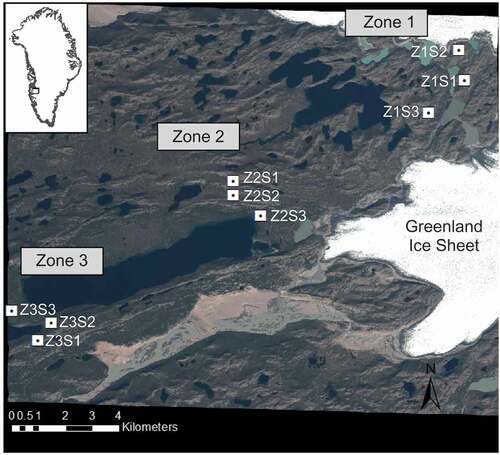
We conducted fieldwork at nine sites in the shrub tundra landscape near Kangerlussuaq, Greenland (Figure 1). The landscape was deglaciated approximately 7,000 years ago (Levy et al. 2012), and is located at the margin of the current extent of the Greenland Ice Sheet (GrIS). The landscape is covered by aeolian silt deposits above bedrock and glacial till (Dijkmans and Törnqvist 1991). Soils are humus-poor arctic brown soil in the soil order Gelisol (Jones et al. 2009). Soil erosion features, termed deflation patches, which are likely a result of strong winds from the GrIS, are common on the landscape and are visually distinct areas with low vegetative cover and productivity (Heindel, Chipman, and Virginia 2015). In addition to geophysical controls, climate and vegetation shifts are likely to be key environmental drivers of biogeochemical cycling in this and other tundra ecosystems. From 1973 to 1999, the average annual atmospheric temperature observed at Kangerlussuaq was −5.7°C (DMI 2017). According to regional climate projections, by the years 2021–2050, atmospheric temperature is projected to increase by 2°C in summer and autumn seasons from historical seasonal averages of 9.2°C and −4.9°C, respectively. Winter is projected to increase by 3°C from a historical mean of −19.2°C, while a 4°C increase from a historical mean of −7.7°C is projected for the spring (DMI [Danish Meterological Institute] 2017; Stendel et al. 2007). Annual precipitation in Kangerlussuaq is approximately 250 mm (Mernild et al. 2015) and is projected to increase 15 percent by 2021–2050 and 30–40 percent by 2051–2080 (Stendel et al. 2007).

Figure 1. Map of the study area, with sites indicated over a WorldView2 satellite image from July 10, 2010. Inset map marks the study area (black rectangle) in west Greenland

Land Cover Classification

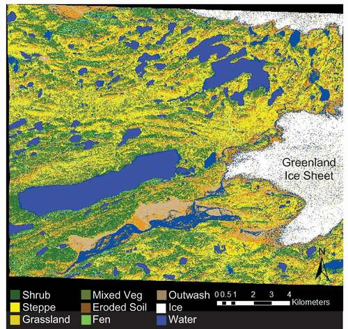
To create a land cover classification map of the study area near Kangerlussuaq, we conducted a multistage unsupervised classification of a WorldView2 image (multispectral, 1.34 m resolution) taken on July 10, 2010. In ENVI Software (Harris Geospatial Solutions) we ran a ISODATA land cover classification to obtain twenty spectral classes with a 5 percent change threshold and a maximum of twenty iterations. Drawing on field knowledge accumulated during the summers of 2010–2013 and visual inspection of the satellite imagery, we visually interpreted the output spectral classes to determine land cover classes based on vegetation functional group. Six spectral classes contained pixels of multiple land cover types, so we built a mask for each mixed class with Spatial Modeler in ERDAS Imagine to isolate the mixed classes. We then ran ISODATA on each masked class with a maximum of eight classes and fifteen iterations. For classes that were split between water and land after the second stage of unsupervised classification, we chose to preserve the integrity of terrestrial land cover. We merged the initial classified and the masked images using Spatial Modeler and simplified the images into nine main classes: shrub, steppe, grassland, mixed vegetation, fen, eroded soil (ES), water, ice, and cloud (Table 1). The ES class includes deflation patches and exposed bedrock, but bedrock is less than 20 percent of unvegetated areas (Heindel, Chipman, and Virginia 2015). To focus on terrestrial classes, we calculated percent cover and total area of shrub, steppe, grassland, mixed vegetation, fen, and ES land cover types by multiplying the number of pixels in each class by the pixel size.

Table 1. Description of cover type used in land classification and field sampling

Cover Type	Common Species	Description
Shrub	Salix glauca Betula nana Rhododendron tomentosum	Dominated by dwarf shrub species
Mixed vegetation	Betula nana Rhododendron groenlandicum Epetrum nigrum	Occurs mainly on damp soil on gently sloping hillsides. Composed of a mix of shrub, with forbs and graminoid undergrowth
Steppe	Calamagrostis purpurascens Carex supina Agrostis mertensii Kobresia myosuroides Potentilla arenosa	Graminoid dominated with scattered forbs, common on south-facing slopes
Eroded soil (ES)	Biological soil crusts Dryas integrifolia Silene acaulis	Common on ridgelines and south-facing slopes, where loess soil has been locally removed by wind erosion: 10–20 percent vegetation cover*
Grassland	Poa pratensis Erophorum angustifolum Calamagrostis lapponica Carex bigelowii Campanula gieseckiana Cerastium alpinum Ranunculus hyperboreus	Found in moist depressions, and are dominated by graminoid species with intermixed forbs
Fen	Carex sp. Eriophorum sp. Hippuris vulgaris	Found along the edge of streams and lakes, and includes shallow lakebeds with ephemeral surface water

*Heindel, Chipman, and Virginia (2015).

We assessed the accuracy of the land cover classification by comparing land cover classes to 288 ground control waypoints from field observations. These points were not used during the development of the classification. We used the ground control points to calculate an error matrix and accuracy statistics for the terrestrial classes in the land classification map.

Site Selection

Study sites for field measurements and soil sample collection were selected from the land cover classification map and ground observations. Three zones were established according to proximity to the margin of the GrIS, where Zone 1 borders the ice edge and Zone 3 is the farthest away, extending toward the fjord Kangerlussuaq (Figure 1). Within each zone we identified five to seven possible sites that each contained representative land cover types (shrub, mixed vegetation, steppe, and ES). Three sites were randomly selected from candidate sites. Grassland was included when present (a total of five sites). Fen samples were collected at one site, Zone 1 Site 2 (Z1S2). We measured air and soil temperature, conducted vegetation surveys, and collected soil samples at all sites, and took in situ soil respiration measurements at seven sites (Table 2).

Table 2. Sample collection and measurement across the study sites. Vegetation types are shrub (SH), steppe (ST), grasslands (GL), mixed vegetation (MX), eroded soil (ES), and fen (FN)

Zone	Site	Air Temperature	No. Soil Temperature Loggers by Vegetation Class				Vegetation Surveys and Soil Samples (2011)	In Situ Soil Respiration (2012)
			SH	ST	MX	ES
1	Z1S1	Yes	3	2	3	3	SH, ST, GL, MX, ES, FN	July 12
	Z1S2	Yes	2	1	3	3	SH, ST, MX, ES	July 12
	Z1S3	Yes	3	2	3	2	SH, ST, GL, MX, ES	N/A
2	Z2S1	No	2	2	3	2	SH, ST, GL, MX, ES	July 13
	Z2S2	Yes	2	2	1	3	SH, ST, GL, MX, ES	July 13
	Z2S3	Yes	1	2	1	3	SH, ST, GL, MX, ES	July 13
3	Z3S1	Yes	3	1	2	3	SH, ST, GL, MX, ES	N/A
	Z3S2	Yes	3	2	3	3	SH, ST, MX, ES	July 14
	Z3S3	Yes	3	2	2	2	SH, ST, MX, ES	July 14

The terrestrial land cover classes used in the land classification and sampling design (shrub, mixed vegetation, steppe, grassland, fen, and ES; Table 1) are comparable to a Landsat-based vegetation classification created to assess caribou habitat (Tamstorf, Aastrup, and Cuyler 2005).

Air and Soil Temperature

At each site, we monitored air and soil temperature every four hours using Thermocron iButton loggers (Model DS 1921G, Embedded Data Systems®). To measure air temperature at each site and capture air temperature patterns across the study area, iButton loggers were installed in PVC capsules with a drilled hole to enable air exchange, attached to rebar at 30 cm height, and shaded under an aluminum roof in an area without shrub cover from July 11, 2011, to August 22, 2012. Soil temperature loggers were buried at 5 cm depth within steppe, shrub, mixed vegetation, and ES land cover types between July 17, 2011, and June 12, 2012. Within each vegetation type, we identified three soil temperature locations by randomly selecting a direction (degrees from true north) and a number of steps from the center point of a continuous patch of land cover. If a patch was smaller than approximately 8 m in diameter, we distributed the temperature loggers among more than one patch. We placed a total of twelve loggers per site, and 108 across the entire study area. The data from twenty-five loggers were not included in analyses because the loggers were either disturbed by wildlife or could not be located, but all vegetation types at each site had at least one logger with a complete data record (Table 2). All temperature loggers were wrapped in parafilm and neoprene plastic for waterproofing.

Vegetation Surveys and Soil Sampling

At each site, we identified a soil pit location at the center of each vegetation type. We avoided vegetation boundaries to maximize the likelihood of collecting soils that have a long-lived association with the vegetation type of interest. Prior to disturbing the soil surface, we conducted a vegetation survey within a 0.5 m² quadrat at each soil pit location. We visually estimated percent cover of shrub, herbaceous, graminoid vegetation using a 0.5 m² quadrant.

We collected soil samples from a 50 cm soil profile using visual classification to sample detectable horizons. At some sites, the active layer was shallower than 50 cm, so we sampled soil to the depth of frozen ground. We collected at least 75 g of soil from each depth interval using a spoon that was cleaned between samples to minimize contamination, and stored samples in separate sterile Whirl-pak® bags (Nasco, Fort Atkinson, WI). Soil samples were frozen and shipped to the Environmental Measurements Lab, Dartmouth College (Hanover, NH) where they were kept at −20°C until processing.

Soil Analyses

Samples were thawed and sieved to isolate the less than 2 mm fraction of each soil horizon for laboratory analysis. Soil water content was estimated from a 10 g soil sample that was dried at 95°C for 24 h, reweighed, and calculated as g water g⁻¹ dry soil. Soil pH was measured using a 1:2 solution of soil:di-H₂O using a pH meter (Thermo Scientific, Orion 3 Star A111 pH Benchtop, Waltham, MA). Electrical conductivity was measured using a 1:5 solution of soil:di-H₂O using a conductivity meter (Thermo Scientific, Orion 3 Star Conductivity Benchtop, Waltham, MA). Carbon and nitrogen content was measured on soils ground with a mortar and pestle using a Carlo Erba NA-1500 elemental analyzer (Carlo Erba Instruments, Milan, Italy) using standard methods (Sollins et al. 1999). Hydrochloric acid was added to samples from mineral soils in vegetated areas to remove inorganic carbonates. No reaction to the hydrochloric acid was visually observed.

In Situ Soil Respiration Measurements

We measured in situ soil respiration (CO₂ flux) with a portable Li-Cor 8100 (Lincoln, NE) infrared gas analyzer (IRGA) with a 20 cm survey chamber attached. At seven of the nine field sites, we installed three 20 cm diameter PVC collars at randomized locations within shrub, steppe, grassland, mixed vegetation, and ES vegetation types. Following installation, collars sat for at least twenty minutes to minimize the effect of physical disturbance on CO₂ diffusion across the soil surface. This time interval was selected based on sampling logistics and a limited number of PVC collars that precluded long-term set up in the sampling required for this particular study. We measured the height of the collar above ground to calculate the volume of the headspace in each PVC ring. In a random order, we recorded the CO₂ flux with a two-minute observation after a twenty-second pre-purge. We collected a total of 106 measurements during a rainless three-day sampling period (July 12–14, 2012). Data were not collected at two sites because of logistical challenges and limited field time: Z1S3 was too remote to access during the survey period, and Z3S1 was an outlier in elevation (354 m vs. 253 m and 264 m for the other Zone 3 sites).

Calculations and Data Analysis

Temperature Analyses

To test our assumption that air temperature increases extending away from the ice sheet, we compared mean annual temperature, growing season temperature, and winter temperature between zones using a multivariate analysis of variance (MANOVA) followed by univariate analysis to test differences within each dependent variable. The annual average was calculated from data recorded between July 11, 2011, and July 10, 2012. We defined growing season as the dates between leaf out and senescence, May 22 to August 7 (Post and Forchhammer 2008; Post and Pedersen 2008), and winter season as the cold season climate window, November 28 to March 27 (Weatherspark 2015). The logger for one site (Z2S1) disappeared during the winter months, so the site was not included in air temperature comparisons.

We compared the soil temperature environment using thermal sum for each logger during the measurement period. Thermal sum is the difference between the recorded temperature above the baseline temperature of 0°C and the baseline, summed for the number of days in the measurement period. We conducted a model comparison of linear mixed effect models to test land cover type, zone, and the interaction between the two as predictor of soil thermal sum, with site as a random variable in the model. A second model comparison was conducted to test land cover type, zone, and their interaction as predictors of thermal sum of soils in vegetated land cover types, excluding the soil land cover type. We used Tukey’s HSD (α = 0.05) to evaluate differences between means, and calculated marginal R², a measure of variance for mixed effect models.

Soil Chemistry Ordination

We conducted multivariate analysis to test whether soil chemistry differed by vegetation type and zone. Measures of percent organic C, percent N, C:N, pH, EC, and soil water content were used in a partial redundancy analysis (RDA) to determine if these variables differed by vegetation type and zone (vegan package in R [Oksanen et al. 2015]). RDA provides a quantitative method of testing hypotheses in multidimensional datasets. Each soil sample is assigned scores on constrained axes of the predictor variables and unconstrained axes to account for the remaining variance. Soil chemistry measures were used as response variables. Vegetation type and zone were used as predictor variables, with depth as a covariate in the model. Eight soil samples were not included in the analysis because the sample did not contain enough soil mass to conduct a full set of soil chemistry measurements. We analyzed a total of 239 soil samples. The response variables were standardized using the scale function to reduce the influence of the magnitude of model variables on the association between samples. A permutations test with 5,000 permutations was used to determine if vegetation type and zone explained a significant portion of the variance in soil chemistry between samples. Adjusted R² was calculated to partition variance between the explanatory and covariate variables (Borcard, Gillet, and Legendre 2011).

Soil Carbon Pools and Landscape Storage

We estimated the organic carbon pool for near-surface soil (0–20 cm depth) and the full active layer profile up to 50 cm depth (Equation 1(1) $\begin{array}{rl}& \mathrm{S}\mathrm{O}\mathrm{C}\left(\mathrm{k}\mathrm{g}\mathrm{C}{\mathrm{m}}^{-2}\right)=\mathrm{\%}\mathrm{C}\times {\mathrm{D}}_{\mathrm{b}}\times \mathrm{d}\times 10^4\mathrm{c}{\mathrm{m}}^2{\mathrm{m}}^{-2}\\ & \times 10^{-3}\mathrm{k}\mathrm{g}{\mathrm{g}}^{-1}\end{array}$(1) ):

(1) $\begin{array}{rl}& \mathrm{S}\mathrm{O}\mathrm{C}\left(\mathrm{k}\mathrm{g}\mathrm{C}{\mathrm{m}}^{-2}\right)=\mathrm{\%}\mathrm{C}\times {\mathrm{D}}_{\mathrm{b}}\times \mathrm{d}\times 10^4\mathrm{c}{\mathrm{m}}^2{\mathrm{m}}^{-2}\\ & \times 10^{-3}\mathrm{k}\mathrm{g}{\mathrm{g}}^{-1}\end{array}$(1)

where % C is SOC concentration, D_b is bulk density (g soil × cm⁻³), and d is depth (cm). We assigned bulk density to soil horizon and depth based on measurements from other studies that we conducted in the same area and vegetation types, with bulk densities of 0.25 g DW cm⁻³ for organic soils (Bradley-Cook and Virginia 2016), 0.62 g DW cm⁻³ for shallow mineral soils (<10 cm depth), and 1.37 g DW cm⁻³ for deeper mineral soils (10–20 cm; Petrenko et al. 2016). We estimated soil nitrogen pools with identical calculations from percent N. We calculated terrestrial soil carbon and nitrogen inventories at the landscape scale by multiplying soil carbon content by area in the land cover classification map for each terrestrial class.

We used linear mixed effects models to test zone and vegetation type as predictor of soil carbon stocks of the full soil profile. We identified significant differences between vegetation types using Tukey’s HSD test in the multcomp package in R. Carbon and nitrogen areal stocks were log-transformed to meet assumptions of normality and homoscedasticity. We back-transformed the mean and the 95 percent confidence interval values (Hanlon and Larget 2011).

Results

Land Cover Classification

The land cover classification contains nine land cover classes: shrub, steppe, grassland, mixed vegetation, eroded soil (ES), fen, water, fluvial sediment (outwash) and ice (Figure 2). Ground-based vegetation surveys at 288 points reveal that the classification has an overall accuracy of 50 percent. Producer’s accuracy, which provides the probability that a pixel in the classification corresponds with the correct vegetation type, was as high as 84 percent in the ES class and as low as 17 percent in the fen class (Table 3). User’s accuracy, or the probability that the cover type at a single point corresponds with the land cover class on the map, ranged from 20 percent for fen to 60 percent for grassland. The most dominant land cover type of the terrestrial landscape was steppe (25%), and is closely followed by mixed vegetation (22%), ES (22%), and shrub (19%; Table 4). The least common land cover types were grassland (7%) and fen (5%; Table 4).

Table 3. Error matrix comparing land cover classes from satellite classification with ground-based vegetation observations. Vegetation classes are shrub (SH), steppe (ST), grassland (GL), mixed vegetation (MX), eroded soil (ES), fen (FN), and water (W)

		Ground Control Data
		SH	ST	GL	MX	ES	F	W	Row Total
Classification by satellite image	SH	21	7	1	17	3	0	0	49
	ST	12	34	2	8	8	1	0	65
	GL	5	17	6	4	0	0	0	32
	MX	21	8	1	35	3	3	0	71
	ES	2	7	0	0	47	0	0	56
	FN	4	0	0	0	1	1	0	6
	W	1	0	0	0	8	0	0	9
Column total		66	73	10	64	70	5	0	288
Producer accuracy				User accuracy
SH	43%	SH	32%
ST	52%	ST	47%
GL	19%	GL	60%
MX	49%	MX	55%
ES	84%	ES	67%
FN	17%	FN	20%
Overall accuracy		50%

Table 4. Area, percent cover, carbon and nitrogen pools for each terrestrial land cover class. Area was extracted from the land cover classification. Pool sizes are mean values

Land Cover Class	Mean C 20-cm (kg m^−2)	Mean C 50-cm (kg m^−2)	Area (km^2 (%))	Total C 20-cm (Gg C (%))	Total C 50-cm (Gg C (%))
(A) Organic Carbon
Shrub	6.44	14.67	16.13 (19%)	103.86 (16%)	236.59 (17%)
Steppe	8.98	20.17	21.16 (25%)	189.91 (30%)	426.78 (31%)
Grassland	19.07	34.87	5.60 (7%)	106.86 (17%)	195.35 (14%)
Mixed veg	6.71	15.13	18.12 (22%)	121.66 (19%)	274.26 (20%)
Eroded soil	0.46	0.70	18.63 (22%)	8.48 (1%)	13.02 (1%)
Fen	24.36	54.55	4.22 (5%)	102.91 (16%)	230.44 (17%)
TOTAL	–	–	83.86	633.68	1,376.45
(B) Total Nitrogen
Shrub	0.32	0.75	16.13 (19%)	5.21 (13%)	12.13 (14%)
Steppe	0.59	1.33	21.16 (25%)	12.54 (30%)	28.12 (31%)
Grassland	1.30	2.30	5.60 (7%)	7.27 (18%)	12.87 (14%)
Mixed veg	0.36	0.82	18.12 (22%)	6.54 (16%)	14.88 (17%)
Eroded soil	0.04	0.06	18.63 (22%)	0.80 (2%)	1.12 (1%)
Fen	2.13	4.85	4.22 (5%)	9 (22%)	20.49(23%)
TOTAL	–	–	83.86	41.36	89.62

Figure 2. Land cover classification map of the study area. Colors coincide with land cover classes, including the following vegetation classes: shrub, steppe, grassland, mixed vegetation, eroded soil, and fen

Air Temperature

There was a statistically significant difference in air temperature regime between the three zones (F_1,6 = 7.56, P = 0.041; Wilk’s Λ = 0.1508) for the full measurement period, July 11, 2011, to August 22, 2012. Growing season temperatures were significantly different by zone (F_1,6 = 9.335, P = 0.02). Zone 1 had a lower growing season temperature (mean = 9.0°C) than Zone 3 (mean = 11.2°C; Tukey’s HSD P = 0.0586), but not compared to Zone 2 (mean = 10.9°C; Tukey’s HSD P = 0.135). Growing season temperatures of Zone 2 and Zone 3 were not significantly different (Tukey’s HSD P = 0.914). Annual temperatures did not differ by zone (F_1,6 = 3.727, P = 0.102), with a mean annual air temperature for all sites of −3.1°C. Winter temperatures also did not differ between zones (F_1,6 = 0.128, P = 0.733), with a mean temperature of −17.3°C. Thermal sum was significantly different by zone (F_1,6 = 10.377, P = 0.018), with lower thermal sums at Zone 1 (mean = 1084.1 degree days, °Cd) than Zone 3 (mean = 1338.8 °Cd; Tukey’s HSD P = 0.0585; Figure 3). Thermal sum at Zone 2 (mean = 1274.0 °Cd) did not differ from Zone 1 (P = 0.191) or Zone 3 (P = 0.770; Figure 3).

Figure 3. Thermal sums of (A) air and (B) soil temperatures at 5 cm depth in different vegetation types and in three zones. Data points mark site averages with error bars indicating ±1 standard error. Thermal sum of air temperature was calculated for one year (July 12, 2011–July 11, 2012), and soil temperature was calculated between July 17, 2011, and June 12, 2012. Shapes of soil thermal sums indicate vegetation cover (ES = eroded soil, ST = steppe, MX = mixed vegetation, SH = shrub)

Soil Temperature

Land cover type and zone explained a significant amount of the variance in soil thermal sum (Table 5). ES had higher thermal sums than all other land cover classes at all zones (Figure 3). Thermal sums are reduced by more than 400 degree days in vegetated areas (Figure 3). Mean thermal sums of steppe soils have a narrow range of values across all zones (mean = 183°Cd, min = 171°Cd, max = 205°Cd). Shrub soils have lowest thermal sums in Zone 2 (Zone 1 = 298°Cd, Zone 2 = 94°Cd, Zone 3 = 395°Cd). Thermal sum in mixed vegetation decreases moving away from the ice sheet (Zone 1 = 308°Cd, Zone 2 = 153°Cd Zone 3 = 119°Cd).

Table 5. Comparison of models explaining soil thermal sums. The preferred model (ΔAICc < 2) contains an interaction between vegetation type and zone. Site was included as a random variable in all models. Marginal R² of the best fitting model was 0.8116 (Veg = Vegetation)

Rank	Predictor Variable	k	AICc	ΔAICc	AICc Model Weight	Log-likelihood Log(L)
1	Veg + Zone + Veg: Zone	14	1120.4	0.0	1	−543.1
2	Vegetation	6	1132.8	12.4	0	−559.9
3	Vegetation + Zone	8	1134.3	13.9	0	−558.2
4	Intercept	3	1232.7	112.4	0	−613.2
5	Zone	5	1235.8	115.4	0	−612.5

Variation in Soil Organic Carbon, Nitrogen, and Chemistry

The partial RDA examined vegetation and zone as predictors of soil chemistry measurements. The permutation test was significant (F_6,231 = 22.763, P = 0.001). The first two constrained axes were both significant (P < 0.01) and explain 33 percent of the variance, with 25.4 percent attributed to RDA1 and 7.6 percent attributed to RDA2. The remaining constrained axes, RDA3 and RDA4, were not significant (P > 0.05). The correlation variable, soil sample depth, explained 5.2 percent of the variance. The remainder of the variance, 61.4 percent, is unconstrained by vegetation type, zone, or depth.

The permutation test showed that vegetation explains a significant amount of the variation in soil chemistry measurements (F_5,231 = 26.4, P = 0.0002). Zone did not explain a significant amount of the total variance in soil chemistry (F_1,238 = 1.0, P = 0.38).

Total organic carbon, nitrogen, and soil water content were tightly correlated explanatory variables that aligned with the RDA1 axis (Figure 4). Grassland and fen samples had high values along this axis, indicating that the soils have high carbon, nitrogen, and soil water content. Grassland, shrub, and mixed vegetation shared similar position on the RDA1 axis. C:N corresponds with RDA2, and shrub, steppe, and mixed vegetation vary along RDA2, with the highest C:N in shrub soils, the lowest values for steppe soils, and mixed vegetation in an intermediate position.

Figure 4. Ordination biplot of the partial RDA of soil chemistry measurements using vegetation type and zone as the independent variables (Table 6). The centroid of each vegetation type is labeled for shrub (VegSH), mixed vegetation (VegHB), steppe (VegGR), grassland (VegGR2), eroded soil (VegDZ), and fen (VegLA). TOC is total organic carbon, Grav Moist is soil moisture, TN is total nitrogen, EC is electrical conductivity, and PH is pH. The biplot represents 31 percent of the total variance (25.4% on RDA1 and 7.6% on RDA2)

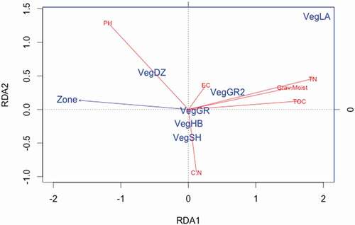
Neither pH nor electrical conductivity were tightly correlated with the RDA axes (Figure 4). ES soils had a strong correlation with pH (Figure 4), with higher pH measurements than the other vegetation types (Table 6). Electrical conductivity varied substantially for all vegetation types, and did not have a strong association with vegetation types or the other chemical measurements.

Table 6. Mean and range of soil chemistry measurements collected from six different vegetation types: N is the number of soil samples, %C is organic carbon content, %N is nitrogen content, SWC is soil water content (g H₂O g Soil⁻¹), and EC is electrical conductivity (micro-siemens cm⁻¹)

Land Cover Class	N	%C	%N	C:N	pH	EC	SWC
Eroded soil	50	0.2 (0.01–1.0)	0.02 (0–0.08)	13.1 (3.6–45.7)	7.6 (5.8–8.6)	51 (2–1648)	2.9 (0.09–7.05)
Steppe	55	5.5 (0.2–21.6)	0.37 (0.01–1.38)	15.2 (8.5–25.3)	6.4 (5.8–7.6)	39 (4–228)	44.6 (2.2–138.5)
Grassland	27	10.2 (0.5–27.5)	0.66 (0.04–1.63)	15.4 (12.3–19.8)	6.3 (5.1–7.4)	94 (7–594)	82.3 (3.61–381.4)
Mixed vegetation	50	4.6 (0.2–12.9)	0.25 (0.02–0.66)	17.8 (8.5–29.1)	6.4 (5.4–7.2)	26.6 (3–314)	34 (4–80)
Fen	5	22.7 (20.3–26.3)	1.99 (1.81–2.26)	11.4 (11.0–11.7)	6.3 (6.1–6.6)	135 (52–323)	189.1 (178–205)
Shrub	60	4.0 (0.2–20.5)	0.21 (0.01–0.99)	19.7 (6.3–51.4)	6.3 (4.9–7.6)	25 (2–129)	23.4 (3.84–71.7)

Soil C and N Storage by Vegetation Type

Soil carbon stocks varied among land cover types. In the prediction of soil carbon stocks, the best-ranked model (ΔAICc < 2) contained vegetation type as the only predictor (Table 7). Grassland soils and the single fen sample contained the highest mean carbon stocks (mean, 95% CI: 34.87 kg C m⁻², [27.30, 44.55] and 54.55 kg C m⁻², respectively; Figure 5). Steppe (mean, 95% CI: 20.17 kg C m⁻², [12.64, 32.18]), mixed vegetation (mean, 95% CI: 15.13 kg C m⁻², [9.50, 24.11]), and shrub (mean, 95% CI: 14.67 kg C m⁻², [9.80, 21.95]) soil carbon storage were not significantly different from one another (Figure 5). ES areas had the lowest carbon storage (mean, 95% CI: 0.07 kg C m⁻², [0.46, 1.07]; Figure 5).

Table 7. Comparison of models explaining soil organic carbon stocks. The top-ranked model, with vegetation as a main effect, is preferred. All other models, ΔAICc > 2

Rank	Predictor Variable	k	AICc	ΔAICc	AICc Model Weight	Log-likelihood Log(L)
1	Vegetation	7	276.97	0	0.80	−129.8
2	Vegetation + Zone	8	297.75	2.78	0.20	−129.7
3	Veg + Zone + Veg: Zone	12	286.90	9.93	0.01	−129.1
4	Intercept	2	297.93	21.01	0.00	−146.8
5	Zone	3	298.72	21.75	0.00	−146.0

Figure 5. Soil (A) organic carbon and (B) nitrogen pools to a depth of 50 cm for soils from six vegetated land cover types in western Greenland (ES = eroded soil, ST = steppe, GL = grasslands, MX = mixed vegetation, FN = fen, SH = shrub). Horizontal tabs mark the mean of each vegetation type, with error bars that represent ±1 standard error of the mean. Gray data points are the carbon stocks from each soil pit. Different letters indicate significant differences in Tukey HSD post hoc test (P < 0.05)

Mean nitrogen stocks in soils ranged from 0.06 to 4.85 kg N m⁻². As in the prediction of soil carbon, vegetation type was the only predictor term in the best model of soil nitrogen stocks (Table 8). The highest average N stock was in the single fen soil profile (4.85 kg N m⁻²; Figure 5), and grasslands also had elevated N stocks (mean, 95% CI: 2.30 kg N m⁻², [1.60, 3.30]). Steppe (mean, 95% CI: 1.33 kg N m⁻², [0.76, 2.32]), mixed vegetation (mean, 95% CI: 0.82 kg N m⁻², [0.50, 1.34]), and shrub (mean, 95% CI: 0.75 kg N m⁻², [0.47, 1.19]) were not significantly different (Figure 5). ES areas had the lowest nitrogen stocks of all land cover types (mean, 95% CI: 0.06 kg N m⁻², [0.04, 0.09]; Figure 5).

Table 8. Comparison of models explaining soil nitrogen stocks. The top-ranked model, with vegetation as a main effect, is preferred. All other models, ΔAICc > 2

Rank	Predictor Variable	k	AICc	ΔAICc	AICc Model Weight	Log-likelihood Log(L)
1	Vegetation	7	54.38	0	0.75	−18.5
2	Vegetation + Zone	8	56.68	2.31	0.24	−18.2
3	Veg + Zone + Veg:Zone	12	62.08	7.71	0.02	−13.7
4	Zone	3	78.66	24.28	0.00	−36.0
5	Intercept	2	78.83	24.45	0.00	−37.3

Soil Carbon Respiration by Vegetation Type

Soil carbon respiration rates during the mid-season differed by vegetation type (Figure 6). The highest respiration was observed in grassland vegetation, with an average rate of 7.10 ± 0.60 μmols CO₂ m⁻² s⁻¹, which was significantly greater than all other vegetation types (P < 0.05). Average soil respiration for steppe, shrub, and mixed vegetation ranged from 3.11 to 3.42 μmols CO₂ m ⁻² s⁻¹, but did not significantly differ from each other. In ES, average respiration rate was an order of magnitude lower than grasslands (0.69 ± 0.45 μmols CO₂ m⁻² s⁻¹).

Figure 6. Average soil respiration rates in five vegetation types during the growing season. Error bars are ±1 standard error around the mean. Different letters indicate significant difference in Tukey HSD post hoc test (P < 0.05)

Landscape Soil Carbon and Nitrogen Estimates

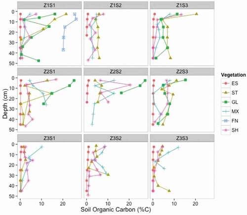
The terrestrial landscape stores an average of 16.41 kg C m⁻² in the active layer soils to a depth of 50 cm. Approximately 46 percent of this carbon is stored in the 0–20 cm depth increment, with an average of 7.4 kg C m⁻² for the top 20 cm of soil. Several soil profiles had elevated carbon content in the deepest sample collected (e.g., Z1S1-GL [grassland], Z3S2-ST [steppe], Z3S3-MX [mixed vegetation], and Z3S3-ST [steppe]; Figure 7).

Figure 7. Soil organic carbon content (%) for each soil profile. Symbols correspond to the vegetation types (ES = eroded soil, ST = steppe, GL = grasslands, MX = mixed vegetation, FN = fen, SH = shrub). Profiles are grouped by sites in each panel, with Zone 1 sites in the top row, Zone 2 sites in the middle row, and Zone 3 sites in the bottom row

Steppe and mixed vegetation comprise the largest fraction of total landscape carbon (31% and 20%, respectively; Table 4). Fen and grassland make up 17 percent and 14 percent, respectively, even though they cover the smallest fraction of the landscape area (5% and 7%, respectively; Table 4). An estimated 17 percent of landscape carbon is stored in shrub soils. ES areas, which cover 22 percent of the landscape area, only store 1 percent of the total carbon in the landscape (Table 4).

Nitrogen stocks in the terrestrial landscape are 1.07 Gg N m⁻² in the full soil profile. Near-surface soils store 46 percent of total nitrogen, with an average of 0.49 Gg N m⁻² in the top 20 cm. The largest nitrogen stock is in steppe (31%), which is more than double that of shrub (14%; Table 4). Fen soils store 23 percent of landscape nitrogen, which is disproportionately high when considering it covers only 5 percent of the landscape (Table 4). ES only stores 1 percent of the total landscape nitrogen.

Discussion

Landscape Temperature Variation

Temperature regimes vary with proximity to the ice sheet. Within the study area, which captured a distance of approximately 11 km from the GrIS margin, the influence of the GrIS on atmospheric temperatures is apparent during summer months, but does not have an effect during the winter or at an annual scale. The 2°C cooler growing season temperatures near the margin of the GrIS can have ecological consequences, including altered carbon cycling. Lower temperatures decrease net primary productivity and microbial activity, resulting in a slower cycling of carbon (Chapin et al. 2009).

Regional climate models project that warming will be greatest during the winter season, and will be limited to approximately 2°C warming during the summer months because of a cooling effect from the GrIS (Stendel et al. 2007). Since proximity to the ice sheet does not affect winter temperature within the study area, we infer that projected winter warming of 3°C by 2050 (Stendel et al. 2007) will be experienced equally across the landscape.

The interactive effect of zone and land cover type on soil temperature supported our hypothesis that vegetation is an important mediator of the belowground abiotic conditions. When vegetation is present, soil and atmospheric temperatures are decoupled to an extent. In the minimally vegetated ES, the soil temperature is more tightly linked to air temperature as observed by the increase in temperature with distance away from the ice sheet. The largest differences in thermal sums were between ES and vegetated areas. Differences within vegetation types were smaller. These results indicate that soil temperature is associated with vegetation, and that vegetation could mediate the impact of climate change on belowground abiotic conditions and biological response. Other studies have found vegetation to be an important determinant of soil temperature (Aalto, Le Roux, and Luoto 2013; Migala et al. 2014) that can alter heat exchange from warming (Hollister et al. 2006), which adds uncertainty to modeling soil organic carbon response to climate change (Xiong et al. 2015).

Heterogeneity in Land Cover Class

The high heterogeneity of land cover types at small spatial scales would decrease the overall accuracy of the land cover classification. Our ground control points were within the nine field sites, which were chosen because they had representative land cover classes within close proximity to each other. As a result, many of the vegetation patches were small (size ranged from 3 m to 40 m in diameter) and close to boundaries with other vegetation types. In these conditions, error from handheld GPS units combined with any small georeferencing errors can easily propagate and result in a misalignment of ground control points and the land cover classification and reduced accuracy metrics. The ES class, with a distinct spectral signal from vegetation, had a producer accuracy of 84 percent, which we consider to be fairly high given the possibility of error propagation mentioned above. Grassland and fen vegetation had the lowest producer accuracy (Table 3), likely because these features are commonly confined to small areas on the landscape and therefore have a higher likelihood of accumulating error in the accuracy assessment process. Improvements in the accuracy metrics of our classification might be gained by the addition of randomly generated ground control data points that are at least three meters away from a vegetation boundary. The buffer around the data point should reduce the influence of instrument error.

Heindel, Chipman, and Virginia (2015) also conducted a land cover classification of an overlapping, but larger, study area. Their land cover composition estimates were comparable to ours. We attribute discrepancies in direct comparison of our estimates to the fact that their study area extended farther west than ours, thus included a greater proportion of land where wind erosion features are less common. These landscape classification maps are useful tools for the scaling of ecological variables such as soil carbon and nitrogen stocks and are reflective of the natural variability in the landscape.

Soil Chemistry Variation

Multivariate analysis of the soil chemistry revealed that carbon, nitrogen, and soil moisture are the constrained variables associated with most of the variation among soil samples. Soil C, N, and moisture are highly correlated in other arctic terrestrial systems (e.g., Hollingsworth et al. 2008) and are likely a result of a positive feedback between soil conditions and primary productivity. Additionally, soil moisture can constrain microbial decomposition when soils are near saturation as a result of limited oxygen availability in the soil matrix. Grasslands and fen soils have high values of C, N, and moisture. Meanwhile, steppe, shrub, and mixed vegetation, which account for a majority of the land cover, have similar position relative to the axis describing the variation in C, N, and moisture, but are differentiated on the second axis, which is associated with the C:N ratio. These results support our hypothesis and other studies that shrub soils have higher C:N than graminoid-dominated soils, and the mixed vegetation ratio reflects a mixture of C:N inputs and places these soils at an intermediate position. Higher C:N in shrub soils has also been found in mineral soils in the study area (Petrenko et al. 2016). The same shrub soils also have reduced soil respiration potential and temperature sensitivity compared to adjacent grassland soils, which may be a result of nutrient limitation on decomposition from lower nitrogen stocks in shrub soils (Bradley-Cook et al. 2016). ES have the lowest position on the axis associated with C, N, and moisture (RCA1), which indicate that these soils have limited biological development. These soils also have a higher pH than other vegetation types, highlighting that they have a unique chemical profile that could further limit enzymatic activity and microbial decomposition (Min et al. 2014).

Distribution of Soil Organic Carbon at a Landscape Scale

The landscape-wide average carbon stock weighted by area is 16.41 kg C m⁻², which is within the estimate assigned to west Greenland in the regional assessments of soil organic carbon, 10–25 kg C m⁻² (Hugelius et al. 2013). This average carbon stock is greater than that of high Arctic field sites near Thule, Greenland, where striped patterned ground soil contains SOC content of 9.4 kg C m⁻² (Horwath et al. 2008). Other prominent Arctic field areas, such as Toolik Lake Field Station on the north slope of Alaska and Svalbard, have higher SOC stocks that fall in the 25–50 kg C m⁻² range (Hugelius et al. 2013).

Soil carbon content varied across the landscape, and has statistically significant associations with land cover type. The highest carbon stocks of the vegetation classes sampled at multiple sites are associated with grasslands, with an average of 34.87 kg C m⁻². Petrenko et al. (2016) estimated mineral soil carbon stocks from grassland soils to be 29 kg C m⁻², which is probably slightly below our estimate because they focused on mineral soil C dynamics and did not include the surface organic horizon in their analysis. Grassland vegetation types only comprise 7 percent of the total study area, but it contains approximately 15 percent of the landscape soil carbon stock. The elevated in situ respiration rates from grassland soils correspond with laboratory measurements of carbon mineralization in which grassland soils have a 1.8 times higher soil respiration than shrub soils (Bradley-Cook et al. 2016). Together, these findings indicate that, in this landscape, grasslands are hot spots for mid-summer soil respiration and for soil carbon storage. The pattern in soil carbon storage suggests that soil carbon inputs from plant production have exceeded soil carbon losses from respiration over a long time frame. Soil respiration rates, however, capture instantaneous dynamics, so the strength of the carbon sink may be different than in the past. It is possible that recent atmospheric warming has elevated carbon losses relative to uptake and storage.

The single fen soil profile measured had a soil carbon stock of 54.6 kg C m⁻², which is the highest stock measured of all soil pits in this study. Anderson et al. (2009) found lake sediments in the Kangerlussuaq region to contain large carbon stocks (an average of 42 kg C m⁻²) and suggest that these low-lying, mostly saturated soils are the most carbon-rich areas in the landscape. The high carbon content of these soils, combined with seasonally dynamic hydrology, indicates that soils such as these could be an important contributor to the landscape dynamics of the CO₂ and CH₄ exchange between the terrestrial ecosystem and the atmosphere.

The most common vegetation types were ranked lowest with respect to carbon stock per unit area. While the average carbon stocks of steppe, shrub, and mixed vegetation are at least 40 percent lower than grassland, they comprise a substantial portion (approximately 68%) of total landscape storage because of their areal extent. Estimates of near-surface shrub carbon stocks (Table 5) are within the range of comparable measurements in the study area, 3.07–7.67 kg C m⁻² (Bradley-Cook and Virginia 2016) and to shrub tundra stocks measured in Siberia, 7.1–7.8 kg C m⁻² (Hugelius and Kuhry 2009). Many studies in Arctic tundra systems, which were conducted in low-lying tundra, have focused on fen and bog hot spots instead of soils with lower carbon stocks, because these features are common and comprise a majority of the carbon stocks (e.g., Hugelius and Kuhry 2009). However, in systems such as Kangerlussuaq, characterized by steep terrain and semiarid conditions, low-lying grassland and fen vegetation cover a relatively small proportion of the area. From our landscape-level analysis of total soil carbon storage by vegetation type, we found that even though shrub, steppe, and mixed vegetation have lower carbon stocks per unit area (i.e., kg C m⁻² values) than fen and grassland, they collectively store most of the total soil organic carbon (i.e., kg C values) because they comprise a majority of the total vegetation cover. Thus, shrub, steppe, and mixed vegetation are biogeochemically important partitions of the Kangerlussuaq tundra landscape.

Landscape Carbon Storage Response to Environmental Change

To investigate the possible trajectory of soil carbon stocks in response to vegetation and climate drivers at the landscape scale, we considered the impact of shrub expansion and climate warming scenarios on landscape soil carbon. Given the assumption that a vegetation shift is accompanied by a corresponding shift in soil properties, shrub expansion and prolonged occupation into graminoid-dominated areas (steppe and grassland) should result in a shift from the high carbon, low C:N soils associated with grassland vegetation to the lower carbon, high C:N soils associated with shrub vegetation. One possible mechanism for this potential shift is that shrub expansion could increase winter soil respiration and soil nitrogen mobilization as predicted by the snow-shrub interaction hypothesis (Sturm, Holmgren, and McFadden 2001; Sturm et al. 2005). Under this scenario, a shift to greater shrubiness would reduce the landscape soil carbon stock and increase soil C:N. However, it is also possible that the general characteristics of graminoid soils could be preserved under shrub expansion scenarios. Total landscape carbon storage will be a function of the net change in soil and vegetation carbon stocks. While the vegetation carbon stock increases with shrub expansion, this component of Arctic terrestrial carbon stock is a small percentage of soil carbon stocks (McGuire et al. 2009), which suggests that the net change will be driven by soil carbon response to climate change. Our data show that growing season soil respiration and soil moisture are lower in shrub soils. If these factors constrain soil carbon efflux we could expect to see a legacy effect of graminoid soils that could contribute to SOC heterogeneity associated with shrub vegetation under projected vegetation change scenarios.

The carbon losses associated with shrub expansion could be compounded with a warming climate. Microbial decomposition most often increases with temperature, and the rate of increase can vary between soils. Previous research on soils in this study area shows that the temperature sensitivity of decomposition is higher in grasslands than shrub soils (Q-10_grasslands = 2.3, Q-10_shrub = 1.8), and that soil moisture increases respiration in grassland soils but not shrub soils (Bradley-Cook et al. 2016). These known temperature sensitivities suggest that SOC decomposition rates will accelerate with warming for both shrub and grassland soils, so increased soil respiration can be expected under any vegetation scenario.

Climate change is a key driver of shrub expansion in tundra ecosystems (Myers-Smith et al. 2011), so it is likely that atmospheric warming and shrub expansion will co-occur. However, as our findings indicate, vegetation mediates the relationship between air and soil temperature, so atmospheric warming may not result in a concomitant increase in soil temperature. For instance, shrub canopy shading can have a local cooling effect on soil temperatures (Jean and Payette 2014; Sturm, Holmgren, and McFadden 2001). We did not observe differences in soil temperature between shrub and graminoid vegetation, so it is possible that canopy shading does not have a sufficient effect on insulation to modify soil temperature in the low shrub tundra of this study area (Hollingsworth et al. 2008). It is also possible that other factors, such as aspect, insulation from understory moss, or plant structural feature such as leaf area index, have a stronger effect on soil temperature than small changes in solar insolation. In summary, we posit that landscape soil carbon storage is sensitive to both vegetation change and climate warming, with possible compounding impacts on soil carbon storage in a future in which these changes may occur concurrently.

Conclusions

The Kangerlussuaq tundra landscape has heterogeneous land cover and a growing season air temperature gradient extending from the GrIS. We estimate average landscape carbon stock to be 16.41 kg C m⁻² and nitrogen stock to be 1.07 kg N m⁻². We found differences in carbon stocks and soil respiration by vegetation type, with enhanced carbon storage and soil respiration in grassland soils. Combined with the understanding that these soils are more sensitive to temperature and moisture, we conclude that grasslands are highly sensitive hot spots of soil carbon storage and mid-growing season soil respiration within a shrub-dominated matrix. Even though shrub, steppe, and mixed vegetation have lower carbon stocks per unit area, they are still important components of landscape-level biogeochemical cycling because they cover more than 50 percent of the area. Shrub expansion into graminoid-dominated areas could possibly result in lower landscape soil carbon storage in the long term. Warming could drive compounding losses of stored carbon, although organic carbon may be more stable in shrub soils, where decomposition rates are less temperature sensitive than in grassland soils. However, vegetation mediation of air temperature adds uncertainty to the effect of climate change on belowground temperature affects on carbon cycling. These landscape-level carbon storage, turnover, and sensitivities indicate that climate drivers and vegetation dynamics will likely lead to a loss of stored soil carbon and an increase of greenhouse gases flux into the atmosphere.

Acknowledgments

We are deeply grateful to Courtney Hammond Wagner and Ruth Heindel for superb field assistance, to Leehi Yona for helping with sample processing and analysis, and to Paul Zietz for laboratory support. Furthermore, we thank Amy Burzynski and Jonathan Chipman for contributions to the mapping and spatial analysis, Thomas Kraft for guidance on the ordination analysis, Ruth Heindel for providing comments on the manuscript, and all Virginia Lab members for moral support. We are thankful to CH2M Hill Polar Services for unfaltering logistical support in Kangerlussuaq that enabled productive fieldwork. This research was funded by an NSF grant (Award #: 0801490) to Ross Virginia, with additional support from the Institute of Arctic Studies, in the Dickey Center for International Understanding at Dartmouth.

References

- Aalto, J., P. C. Le Roux, and M. Luoto. 2013. Vegetation mediates soil temperature and moisture in Arctic-Alpine environments. Arctic, Antarctic, and Alpine Research 45:1–17. doi:https://doi.org/10.1657/1938-4246-45.4.429.
- Anderson, N. J., W. D’andrea, and S. C. Fritz. 2009. Holocene carbon burial by lakes in SW Greenland. Global Change Biologic 15:2590–98. doi:https://doi.org/10.1111/j.1365-2486.2009.01942.x.
- Borcard, D., F. Gillet, and P. Legendre. 2011. Numerical ecology with R, 292. New York: Springer.
- Bosatta, E., and G. Ågren. 1999. Soil organic matter quality interpreted thermodynamically. Soil Biology & Biochemistry 31:1889–91.
- Bradley-Cook, J. I., C. L. Petrenko, A. J. Friedland, and R. A. Virginia. 2016. Temperature sensitivity of mineral soil carbon decomposition in shrub and graminoid tundra, west Greenland. Climate Change Responses 1–15. doi:https://doi.org/10.1186/s40665-016-0016-1.
- Bradley-Cook, J. I., and R. A. Virginia. 2016. Soil carbon storage, respiration potential, and organic matter quality across an age and climate gradient in southwestern Greenland. Polar Biology 39:1283–95. doi:https://doi.org/10.1007/s00300-015-1853-2.
- Cahoon, S. M. P., P. F. Sullivan, E. Post, and J. M. Welker. 2011. Large herbivores limit CO2 uptake and suppress carbon cycle responses to warming in West Greenland. Global Change Biologic 18:469–79. doi:https://doi.org/10.1111/j.1365-2486.2011.02528.x.
- Callaghan, T. V., L. Bjorn, F. S. Chapin, Y. Chernov, T. Christensen, B. Huntley, R. Ims, M. Johansson, D. Jolly, S. Jonasson, N. Matveyeva, W. Oechel, N. Panikov, and G. Shaver. 2005. Arctic tundra and polar desert ecosystems. In Arctic climate impact assessment, eds. C. Symon, L. Arris, and B. Heal, 244–352. New York: Cambridge University Press.
- Chapin, F., M. Bret-Harte, S. Hobbie, and H. Zhong. 1996. Plant functional types as predictors of transient responses of arctic vegetation to global change. Journal of Vegetation Science 7:347–58.
- Chapin, F., J. McFarland, A. D. McGuire, E. S. Euskirchen, R. W. Ruess, and K. Kielland. 2009. The changing global carbon cycle: Linking plant-soil carbon dynamics to global consequences. Journal of Ecology 97:840–50. doi:https://doi.org/10.1111/j.1365-2745.2009.01529.x.
- Craine, J., R. Spurr, K. Mclauchlan, and N. Fierer. 2009. Landscape-level variation in temperature sensitivity of soil organic carbon decomposition. Soil Biology & Biochemistry 42:373–75. doi:https://doi.org/10.1016/j.soilbio.2009.10.024.
- Creamer, C. A., T. R. Filley, T. W. Boutton, S. Oleynik, and I. B. Kantola. 2011. Controls on soil carbon accumulation during woody plant encroachment: Evidence from physical fractionation, soil respiration, and 13-C of respired CO2. Soil Biology and Biochemistry 43:1678–87. doi:https://doi.org/10.1016/j.soilbio.2011.04.013.
- Davidson, E. A., and I. A. Janssens. 2006. Temperature sensitivity of soil carbon decomposition and feedbacks to climate change. Nature 440:165–73. doi:https://doi.org/10.1038/nature04514.
- Dijkmans, J., and T. Törnqvist. 1991. Modern periglacial eolian deposits and landforms in the Søndre Strømfjord area, West Greenland and their palaeoenvironmental implications. Meddelelser Om Grønland. Geoscience 25:3–39.
- DMI (Danish Meterological Institute). 2017. Klimanormaler for Grønland, Copenhagen, Denmark. Accessed June 4, 2017. http://www.dmi.dk/groenland/arkiver/klimanormaler/.
- Fierer, N., B. Colman, and J. Schimel. 2006. Predicting the temperature dependence of microbial respiration in soil: A continental-scale analysis. Global Biogeochemical Cycles 20:GB3026. doi:https://doi.org/10.1029/2005GB002644.
- Frost, G. V., and H. E. Epstein. 2014. Tall shrub and tree expansion in Siberian tundra ecotones since the 1960s. Global Change Biology 20:1264–77. doi:https://doi.org/10.1111/gcb.12406.
- Haddix, M. L., A. F. Plante, R. T. Conant, J. Six, J. M. Steinweg, K. Magrini-Bair, R. A. Drijber, S. J. Morris, and E. A. Paul. 2011. The role of soil characteristics on temperature sensitivity of soil organic matter. Soil Science Society Of America Journal 75:56–68. doi:https://doi.org/10.2136/sssaj2010.0118.
- Hanlon, B., and B. Larget. 2011. Assumptions and transformations. Madison, Wisconsin: Department of Statistics. Accessed May 20, 2017. http://www.stat.wisc.edu/~st571-1/11-assumptions-2.pdf.
- Heindel, R. C., J. W. Chipman, and R. A. Virginia. 2015. The spatial distribution and ecological impacts of Aeolian soil erosion in Kangerlussuaq, West Greenland. Annals of the Association of American Geographers 105:875–90. doi:https://doi.org/10.1080/00045608.2015.1059176.
- Hinzman, L. D., C. J. Deal, A. D. McGuire, S. H. Mernild, I. V. Polyakov, and J. E. Walsh. 2013. Trajectory of the Arctic as an integrated system. Ecological Applications 23:1837–68.
- Hobbie, S. 1996. Temperature and plant species control over litter decomposition in Alaskan tundra. Ecological Monographs 66:503–22.
- Hollingsworth, T. N., E. A. G. Schuur, F. S. Chapin III, and M. D. Walker. 2008. Plant community composition as a predictor of regional soil carbon storage in Alaskan Boreal Black Spruce Ecosystems. Ecosystems 11:629–42. doi:https://doi.org/10.1007/s10021-008-9147-y.
- Hollister, R. D., P. J. Webber, F. E. Nelson, and C. E. Tweedie. 2006. Soil thaw and temperature response to air warming varies by plant community: Results from an open-top chamber experiment in northern Alaska. Arctic, Antarctic, and Alpine Research 38:206–15.
- Hooper, D., and P. Vitousek. 1998. Effects of plant composition and diversity on nutrient cycling. Ecological Monographs 68:121–49.
- Horwath Burnham, J., and R. Sletten. 2010. Spatial distribution of soil organic carbon in northwest Greenland and underestimates of high Arctic carbon stores. Global Biogeochemical Cycles 24:GB3012. doi:https://doi.org/10.1029/2009GB003660.
- Horwath, J. L., R. S. Sletten, B. Hagedorn, and B. Hallet. 2008. Spatial and temporal distribution of soil organic carbon in nonsorted striped patterned ground of the High Arctic. Journal Of Geophysical Research-Biogeosciences 113:G03S07. doi:https://doi.org/10.1029/2007JG000511.
- Hudson, J. M. G., G. H. R. Henry, and W. K. Cornwell. 2011. Taller and larger: Shifts in Arctic tundra leaf traits after 16 years of experimental warming. Global Change Biology 17:1013–21. doi:https://doi.org/10.1111/j.1365-2486.2010.02294.x.
- Hugelius, G., and P. Kuhry. 2009. Landscape partitioning and environmental gradient analyses of soil organic carbon in a permafrost environment. Global Biogeochemical Cycles 23:GB3006. doi:https://doi.org/10.1029/2008GB003419.
- Hugelius, G., J. Strauss, S. Zubrzycki, J. W. Harden, E. A. G. Schuur, C.-L. Ping, L. Schirrmeister, G. Grosse, G. J. Michaelson, C. D. Koven, J. A. O’Donnell, B. Elberling, U. Mishra, P. Camill, Z. Yu, J. Palmtag, and P. Kuhry. 2014. Estimated stocks of circumpolar permafrost carbon with quantified uncertainty ranges and identified data gaps. Biogeosciences 11:6573–93. doi:https://doi.org/10.5194/bg-11-6573-2014-supplement.
- Hugelius, G., C. Tarnocai, G. Broll, J. G. Canadell, P. Kuhry, and D. K. Swanson. 2013. The Northern circumpolar soil carbon database: Spatially distributed datasets of soil coverage and soil carbon storage in the northern permafrost regions. Earth Systems Sciences Data 5:3–13. doi:https://doi.org/10.5194/essd-5-3-2013.
- Jean, M., and S. Payette. 2014. Effect of vegetation cover on the ground thermal regime of wooded and non-wooded palsas. Permafrost and Periglacial Processes 25:281–94. doi:https://doi.org/10.1002/ppp.1817.
- Jenny, H. 1941. Factors of soil formation. New York: Dover Publications.
- Jones, A., V. Stolbovoy, C. Tarnocai, G. Broll, O. Spaargaren, and L. Montarella. 2009. Soil Atlas of the Northern Circumpolar Region, 1. Luxembourg: European Commission, Office for Official Publications of the European Communities.
- Jørgensen, R. H., H. Meilby, and J. Kollmann. 2013. Shrub expansion in SW Greenland under modest regional warming: Disentangling effects of human disturbance and grazing. Arctic, Antarctic, and Alpine Research 45:515–25. doi:https://doi.org/10.1657/1938-4246-45.4.515.
- Levy, L. B., M. A. Kelly, J. A. Howley, and R. A. Virginia. 2012. Age of the Ørkendalen moraines, Kangerlussuaq, Greenland: Constraints on the extent of the southwestern margin of the Greenland Ice Sheet during the Holocene. Quaternary Science Reviews 52:1–5. doi:https://doi.org/10.1016/j.quascirev.2012.07.021.
- McGuire, D. A., L. G. Anderson, T. R. Christensen, S. Dallimore, L. Guo, D. J. Hayes, M. Heimann, T. D. Lorenson, R. D. Macdonald, and N. Roulet. 2009. Sensitivity of the carbon cycle in the Arctic to climate change. Ecological Monographs 79:523–55.
- Mernild, S. H., E. Hanna, J. R. McConnell, M. Sigl, A. P. Beckerman, J. C. Yde, J. Cappelen, J. K. Malmros, and K. Steffen. 2015. Greenland precipitation trends in a long-term instrumental climate context (1890–2012): Evaluation of coastal and ice core records. International Journal Climatology 35:303–20. doi:https://doi.org/10.1002/joc.3986.
- Migala, K., B. Wojtun, W. Szymanski, and P. Muskala. 2014. Soil moisture and temperature variation under different types of tundra vegetation during the growing season: A case study from the Fuglebekken catchment, SW Spitsbergen. Catena 116:10–18. doi:https://doi.org/10.1016/j.catena2013.12.007.
- Min, K., C. A. Lehmeier, F. Ballantyne, A. Tatarko, and S. A. Billings. 2014. Differential effects of pH on temperature sensitivity of organic carbon and nitrogen decay. Soil Biology & Biochemistry 76:193–200. doi:https://doi.org/10.1016/j.soilbio.2014.05.021.
- Myers-Smith, I. H., S. C. Elmendorf, P. S. A. Beck, M. Wilmking, M. Hallinger, D. Blok, K. D. Tape, S. A. Rayback, M. Macias-Fauria, B. C. Forbes, J. D. M. Speed, N. Boulanger-Lapointe, C. Rixen, E. Levesque, N. M. Schmidt, C. Baittinger, A. J. Trant, L. Hermanutz, L. S. Collier, M. A. Dawes, T. C. Lantz, S. Weijers, R. H. Jørgensen, A. Buchwal, A. Buras, A. T. Naito, V. Ravolainen, G. Schaepman-Strub, J. A. Wheeler, S. Wipf, K. C. Guay, D. S. Hik, and M. Vellend. 2015. Climate sensitivity of shrub growth across the tundra biome. Nature Climate Change. doi:https://doi.org/10.1038/nclimate2697.
- Myers-Smith, I. H., B. C. Forbes, M. Wilmking, M. Hallinger, T. Lantz, D. Blok, K. D. Tape, M. Macias-Fauria, U. Sass-Klaassen, E. Levesque, S. Boudreau, P. Ropars, L. Hermanutz, A. Trant, L. S. Collier, S. Weijers, J. Rozema, S. A. Rayback, N. M. Schmidt, G. Schaepman-Strub, S. Wipf, C. Rixen, C. B. Menard, S. Venn, S. Goetz, L. Andreu-Hayles, S. Elmendorf, V. Ravolainen, J. Welker, P. Grogan, H. E. Epstein, and D. S. Hik. 2011. Shrub expansion in tundra ecosystems: Dynamics, impacts and research priorities. Environmental Research Letters 6:045509. doi:https://doi.org/10.1088/1748-9326/6/4/045509.
- Myers-Smith, I. H., and D. S. Hik. 2013. Shrub canopies influence soil temperatures but not nutrient dynamics: An experimental test of tundra snow-shrub interactions. Ecology and Evolution 3:3683–700. doi:https://doi.org/10.1002/ece3.710.
- Oksanen, J., F. G. Blanchet, R. Kindt, P. Legendre, P. R. Minchin, R. B. O’Hara, G. L. Simpson, P. Solymos, M. H. H. Stevens, and H. Wagner 2015. vegan: Community ecology package. http://CRAN.R-project.org/package=vegan.
- Ostle, N. J., P. Smith, R. Fisher, F. L. Woodward, J. B. Fisher, J. U. Smith, D. Galbraith, P. Levy, P. Meir, N. P. McNamara, and R. D. Bardgett. 2009. Integrating plant-soil interactions into global carbon cycle models. Journal of Ecology 97:851–63. doi:https://doi.org/10.1111/j.1365-2745.2009.01547.x.
- Petrenko, C. L., J. I. Bradley-Cook, E. M. Lacroix, A. J. Friedland, and R. A. Virginia. 2016. Comparison of carbon and nitrogen storage in mineral soils of graminoid and shrub tundra sites, western Greenland. Arctic Science 2:165–82. doi:https://doi.org/10.1139/as-2015-0023.
- Post, E., and M. C. Forchhammer. 2008. Climate change reduces reproductive success of an Arctic herbivore through trophic mismatch. Philosophical Transactions of the Royal Society B 363:2367–73. doi:https://doi.org/10.1098/rstb.2007.2207.
- Post, E., and C. Pedersen. 2008. Opposing plant community responses to warming with and without herbivores. Proceedings of the National Academy of Sciences 105:12353–58. doi:https://doi.org/10.1073/pnas.0802421105.
- Schmidt, M., M. Torn, S. Abiven, and T. Dittmar. 2011. Persistence of soil organic matter as an ecosystem property. Nature 478:49–56. doi:https://doi.org/10.1038/nature10386.
- Sierra, C. A., S. E. Trumbore, E. A. Davidson, S. Vicca, and I. Janssens. 2015. Sensitivity of decomposition rates of soil organic matter with respect to simultaneous changes in temperature and moisture. Journal Advancement Model Earth Systems 7:335–56. doi:https://doi.org/10.1002/2014MS000358.
- Sollins, P., C. Glassman, E. A. Paul, C. Swanston, K. Lajtha, and J. W. Heil. 1999. C and N Dry Combustion. In Standard Soil Methods for Long-Term Ecological Research, eds. G. P. Robertson, D. C. Coleman, C. Bledsoe, and P. Sollins, 92–95. Oxford: Oxford University Press.
- Stendel, M., J. H. Christensen, G. Aoalgeirsdottir, N. Kliem, and M. Drews. 2007. Regional climate change for Greenland and surrounding seas. Danish Climate Centre Report 07-02, Danish Meteorological Institute, Copenhagen, Denmark, 26. Accessed March 15, 2015. http://978-87-7478-547-7.
- Sturm, M., J. Holmgren, and J. McFadden. 2001. Snow-shrub interactions in Arctic tundra: A hypothesis with climatic implications. Journal of Climate 14:336–44.
- Sturm, M., J. Schimel, G. Michaelson, and J. Welker. 2005. Winter biological processes could help convert arctic tundra to shrubland. BioScience 55:17–26.
- Sullivan, P. F., S. J. T. Arens, R. A. Chimner, and J. M. Welker. 2008. Temperature and microtopography interact to control carbon cycling in a high arctic fen. Ecosystems 11:61–76. doi:https://doi.org/10.1007/s10021-007-9107-y.
- Tamstorf, M. P., P. J. Aastrup, and L. C. Cuyler. 2005. Modelling critical caribou summer ranges in West Greenland. Polar Biology 28:714–24. doi:https://doi.org/10.1007/s00300-005-0731-8.
- Thomsen, I. K., B. M. Petersen, S. Bruun, L. S. Jensen, and B. T. Christensen. 2008. Estimating soil C loss potentials from the C to N ratio. Soil Biology and Biochemistry 40:849–52. doi:https://doi.org/10.1016/j.soilbio.2007.10.002.
- Urban, M., M. Forkel, J. Eberle, C. Huettich, C. Schmullius, and M. Herold. 2014. Pan-Arctic climate and land cover trends derived from multi-variate and multi-scale analyses (1981–2012). Remote Sensing 6:2296–316. doi:https://doi.org/10.3390/rs6032296.
- Weatherspark. 2015. Average Weather For Kangerlussuaq (Søndre Strømfjord), Greenland. Accessed August 6, 2015. https://weatherspark.com/averages/27554/Kangerlussuaq-S-ndre-Str-mfjord-Kitaa-Greenland.
- Xiong, X., S. Grunwald, D. B. Myers, J. Kim, W. G. Harris, and N. Bliznyuk. 2015. Assessing uncertainty in soil organic carbon modeling across a highly heterogeneous landscape. Geoderma 251–252:105–16. doi:https://doi.org/10.1016/j.geoderma.2015.03.028.