The K-transect on the western Greenland Ice Sheet: Surface energy balance (2003–2016)

ABSTRACT

We present thirteen years (2003–2016) of surface energy balance calculations from automatic weather stations (AWS) along the K-transect in west Greenland. Although short in a climatological sense, these time series start to become long enough to provide valuable insight into the interannual variability and drivers of melt in this part of Greenland and into trends in certain components of the surface energy balance. For instance, the data clearly reveal that albedo variations explain most of the interannual melt variability at the higher stations in the accumulation zone. Sensible heat becomes a major heat source for melt in the lower ablation zone, while latent heat modulates annual melt by up to 20 W m⁻². Also, at two locations with the longest uninterrupted time series, we see a decreasing trend of incoming longwave radiation (−1.2 to −1.4 W m⁻² y⁻¹, p < 0.10) concurrent with an increase in incoming shortwave radiation (+2.4 to +3.8 W m⁻² y⁻¹, p < 0.10) during the observation period. This suggests that decreasing cloud cover plays a role in the increased availability of melt energy (+0.7 to +2.2 W m⁻² y⁻¹, not statistically significant at p < 0.10). At the AWS situated around the equilibrium line altitude (ELA), the observed negative trend in albedo is strongest of all stations (−0.0087 y⁻¹), as the ELA moves upward and bare ice becomes exposed. These insights are important for modeling the future response of the ice sheet to continued global warming, which is expected to be dominated by surface processes.

KEYWORDS:

• Greenland
• surface melt
• automatic weather station
• surface energy balance
• albedo

Introduction

Data from automatic weather stations (AWS) operating on the Greenland Ice Sheet (GrIS) are invaluable for weather forecasting, climate monitoring, validation of remote sensing data, and evaluation of climate model output (Cullather et al. 2014; Das et al. 2001; Hall et al. 2012, 2013; Noël et al. 2015; Shuman et al. 2014; Stroeve et al. 2001). When standard observed meteorological parameters (air pressure, wind speed/direction, and near surface air temperature) are complemented with humidity, short- and longwave radiation components, and subsurface temperatures, AWS data can also be used to close the surface energy balance (SEB). Over glacier surfaces, this allows for the calculation of melt energy, a fundamental quantity in cryospheric research. Explicit quantification of the duration of melt and melt rate in Greenland is especially important to validate satellite data (Häkkinen et al. 2014; Nghiem et al. 2012) and to explain recent changes in the thickness and extent of the firn layer covering the ice sheet (Charalampidis et al. 2015; Kuipers Munneke et al. 2015; Machguth et al. 2016). Moreover, since 2009 GrIS mass loss consists of more than 50 percent surface melt and the subsequent runoff of meltwater, rather than increased ice discharge (Enderlin et al. 2014).

To monitor the near-surface climate and SEB of the GrIS, two ice sheet–wide AWS networks are currently operational: the Greenland climate network (GC-Net, 1999–present, Steffen and Box 2001; https.colorado.edu/science/groups/steffen/gcnet/) and the Programme for Monitoring of the Greenland Ice Sheet (PROMICE 2007–present; van As, Fausto, and PROMICE Project Team 2011; http://www.promice.org). With some exceptions, GC-Net stations are situated in the accumulation zone and PROMICE stations in the ablation zone, providing a reasonable coverage of near-surface meteorological conditions over the GrIS. In addition to these two larger networks, a small array of four AWS is operated along the K-transect, situated near Kangerlussuaq, west Greenland (~67° N). The K-transect was initiated in the summer of 1990 as part of the Greenland Ice Margin EXperiment (GIMEX; Oerlemans and Vugts 1993), and consisted of a mass balance stake line running from the tongue of Russell Glacier at the ice sheet margin into the accumulation zone. Because it has been revisited every year since 1990, to date this constitutes the longest (approximately twenty-five years) uninterrupted time series of systematic surface mass balance (SMB) measurements in Greenland (Greuell et al. 2001, 2012; van de Wal et al. 2005). Later, the K-transect was further extended toward the interior, and additional instruments were installed, such as single-frequency GPS receivers to monitor ice velocity (van de Wal et al. 2008, 2015).

AWS are operated at four sites along the K-transect. From the outset, these AWS were designed as research stations rather than support stations for logistic operations and/or weather forecasting. As a consequence, the data are not fed into the Global Telecommunication System (GTS), and they can be used as an independent source for model evaluation. Another design condition was that the collected parameter set should include hemispheric downward and upward solar and terrestrial radiation fluxes to enable closure of the SEB and hence calculation of the melt energy. Even so, calculating the surface melt energy from automated near-surface observations remains challenging because (1) it represents the relatively small residual of multiple large energy fluxes; (2) several of the SEB components, such as the turbulent heat fluxes, are not explicitly measured and must be calculated using parameterizations; and (3) accurate autonomous measurements in an ablation zone are difficult because of tilting instruments, changes with respect to the surface, riming of sensors, and more. That is why SEB closure to quantify Greenland surface melt requires a dedicated AWS data-processing model with an atmospheric and subsurface component (Cullen et al. 2014; Kuipers Munneke et al. 2009; Niwano et al. 2015; van den Broeke, Smeets, and van de Wal 2011).

The accompanying article in this issue (Smeets et al. 2018) provides greater detail about the history of the K-transect AWSs, how their technology evolved, and how the data are corrected; in this article we focus on the time series of SEB components, including melt energy, how they are calculated, evaluated, and how they evolve over time, ending with a summary and conclusions.

Data and methods

Field locations

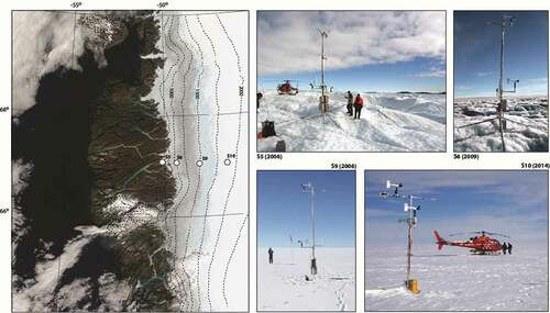
The K-transect starts approximately 20 km east of Kangerlussuaq at the western margin of the GrIS, and runs approximately 140 km eastward over the ice sheet, roughly following the 67°N latitude circle. Currently (June 2017), the K-transect consists of an array of eight SMB stakes, seven single-frequency GPS receivers to determine local ice velocity, and three AWS. Figure 1 shows the three AWS locations: S5 (~490 m a.s.l., 3 km from the ice margin), S6 (~1,050 m a.s.l., 38 km), and S9 (~1,450 m a.s.l., 88 km). AWS S10 (~1,850 m a.s.l., 140 km) was operated until April 2016. Stations S5 and S6 are situated in the ablation zone, where the summer surface consists of bare ice, with a visible dark band running north-south roughly between S6 and S9 (e.g., van de Wal and Oerlemans 1994; Wientjes and Oerlemans 2010; Wientjes et al. 2011). Station S9 is situated close to the long-term equilibrium line, where annual snow accumulation and melt approximately cancel out, and S10 is located in the lower accumulation zone. In the last warm decade, however, the equilibrium line altitude (ELA) has shifted upward significantly; in the warm summer of 2012, it was even situated far above S10 (van de Wal et al. 2012). At S9 and S10, the summer surface consists of wet/refrozen firn. The end-of-summer surface roughness varies from regularly spaced approximately 2–3 m high ice hummocks at S5 to a relatively smooth but metamorphosed snow surface at S10 (Figure 1).

Figure 1. MODIS image of the Kangerlussuaq area, west Greenland. Automatic weather station (AWS) locations given as white circles. Photos demonstrate typical summer conditions at the four AWS locations

Automatic weather stations

At S5, basic AWS data are available from August 1993 to the present day. At S6, data are available since August 1995. However, a full dataset, which is necessary to close the SEB, is only available since August 2003. AWS data from S9 and S10 are available since August 2003 and August 2009, respectively. In April 2009, several months before the initial installation of the AWS at S10, the Geological Survey of Denmark (GEUS) installed a similar AWS (named KAN_U) at this site, as part of the PROMICE network (van As, Fausto, and PROMICE Project Team 2011). Because of extensive experimental activities at S10 focusing on the percolation and refreezing of meltwater in the firn, combined with the harsh local climate conditions, for redundancy it was deemed desirable to have two AWS at this location. The distance between KAN_U and S10 is about 50 m, and the resulting high cross-correlation and small mean differences for each observable allowed us to use KAN_U data to fill twenty-five data gaps in the S10 data series (see the next section) and vice versa. A summary of the climatological setting of each AWS is shown in Table 1.

Table 1. Climatology at the automatic weather stations (AWS) locations for the period August 2003–August 2016. The wind directional constancy is calculated as the ratio of the magnitudes of the average vector and absolute wind speed (from Smeets et al. 2018)

Location	S5	S6	S9	S10
Height (m a.s.l.)	490	1020	1520	1850
Distance from ice edge (km)	6	38	88	140
Wind speed (m s^−1)	3.9	5.1	5.8
Temperature (°C)	−4.1	−8.5	−11.4
Relative humidity (%)	76	87	92
Specific humidity (g kg^−1)	2.1	1.9	1.6
Wind direction (°)	120	124	126
Directional constancy	0.87	0.91	0.82

AWS data

AWS sensors

At S5, S6, and S9, near-surface air temperature T_a, relative humidity RH, and wind speed V are observed at two levels, which are used to estimate the seasonally and annually varying surface roughness length at stations S5 and S6 (van den Broeke et al. 2008). Depending on the sensor type and snow depth, the lower level is at approximately 2–3 m above the surface, and the upper level is at 5–6 m. At S10, where the surface roughness is assumed to be much more constant through the year, a single measurement level at 5–6 m is used. Annual measurement of sensor height in combination with a sonic height ranger, mounted on stakes that are fixed deep into the ice or snow, allows us to accurately reconstruct the snow depth and height of all sensors above the surface at any time. This information is required for the turbulent flux calculations (see further on). All AWS are equipped with a Kipp and Zonen CNR1 radiometer, which measures the four broadband radiation fluxes at 5–6 m height: incoming and reflected solar radiation and down- and upwelling longwave radiation. All observed variables are sampled at 6 min intervals, after which 1 h averages are stored in a Campbell CR10 datalogger. For sensor specifications we refer to Table 2 and to the accompanying article in this issue (Smeets et al. 2018).

Table 2. Sensor type and accuracy of observed variables for all automatic weather stations (AWS) (condensed from Smeets et al. 2018)

Variable	Sensor	Accuracy
Wind speed	05103-L.R.M. Young	0.3 m s^−1
Wind direction	05103-L.R.M. Young	3°
Temperature	Vaisala HMP45C	0.4°C at −20°C
Humidity	Vaisala HMP45C	2% for RH <90%
Net radiation	Kipp Zonen CNR1	10% of daily total
Pressure	Vaisala PTB101B	4 hPa
Surface height	height ranger SR50	0.01 m

Data gaps

The data for this study cover a period of thirteen years, from August 2003 to August 2016. For S5 and S9, an almost continuous data set of hourly SEB input variables is available. Data gaps of one to a few hours are filled by linear interpolation. Data gaps of up to two days are filled using the previous day or days, but this occurred only four times in the entire thirteen-year period. The time series of the AWS at S6 suffers from longer data gaps; sometimes in one, sometimes in all variables. Reasons for the data gaps are diverse, but include battery malfunctioning and instrument and datalogger failure. Small gaps (up to two days) were filled as previously described, but the longer gaps were not filled. As a result, no SEB results for S6 are available for the periods September 2, 2007–September 3, 2008 (367 days); June 10, 2010–August 17, 2010 (70 days); and August 31, 2011–June 12, 2012 (287 days). We used radiation data from the ten preceding and successive days to fill gaps in the radiation data between April 18 and May 9, 2011. By using KAN_U data for the period April–August 2009, the data record for S10 was extended back by an entire melt season. KAN_U data were also used to extend the S10 record from April 2016 to August 2016. From February 2011 to May 2012, both the air and CNR1 temperature data from S10 were corrupted; a combination of S9 and KAN_U temperature data was used to replace the missing observations for this period. Details and more metadata can be found in Smeets et al. (2018).

Data corrections

All data are subjected to a number of data-correction procedures. The most significant corrections are those for air temperature (mainly because of solar radiation heating of the temperature hut at low wind speeds), relative humidity (exhibiting a low-temperature bias), air pressure, wind speed, and wind direction. These correction procedures are detailed in Smeets et al. (2018). The influence of sensor tilt (which can be up to a few degrees in summer) is minimized by using twenty-four-hour accumulated values of SW_in and SW_out to compute net shortwave radiation and albedo (van den Broeke et al. 2004).

Surface energy balance model

The surface energy budget of a snow or ice surface is given by

(1) $\begin{array}{c}\mathrm{M}=\mathrm{S}{\mathrm{W}}_{\mathrm{i}\mathrm{n}}+\mathrm{S}{\mathrm{W}}_{\mathrm{o}\mathrm{u}\mathrm{t}}+\mathrm{L}{\mathrm{W}}_{\mathrm{i}\mathrm{n}}+\mathrm{L}{\mathrm{W}}_{\mathrm{o}\mathrm{u}\mathrm{t}}+\mathrm{H}+\mathrm{L}+\mathrm{G}\\ =\mathrm{S}{\mathrm{W}}_{\mathrm{n}\mathrm{e}\mathrm{t}}+\mathrm{L}{\mathrm{W}}_{\mathrm{n}\mathrm{e}\mathrm{t}}+\mathrm{H}+\mathrm{L}+\mathrm{G}\\ ={\mathrm{R}}_{\mathrm{n}\mathrm{e}\mathrm{t}}+\mathrm{H}+\mathrm{L}+\mathrm{G}\end{array}$(1)

where SW_in, SW_out, LW_in, and LW_out are the incoming and outgoing shortwave (SW) and longwave (LW) radiation components, H and L are the turbulent fluxes of sensible and latent heat, G is the surface value of the subsurface (conductive) heat flux, and M is the melt flux. All energy fluxes are in W m⁻² and defined positive when directed toward the surface.

H and L are calculated using the bulk formulation of the flux-profile relations:

(2) $\mathrm{H}=\rho {\mathrm{c}}_{\mathrm{p}}{\mathrm{u}}_{\ast }{\theta }_{\ast }$(2)

(3) $\mathrm{L}=\rho {\mathrm{L}}_{\mathrm{s}}{\mathrm{u}}_{\ast }{\mathrm{q}}_{\ast }$(3)

Here, u_*, θ_*, and q_* are the turbulent scales of vertical velocity, potential temperature, and specific humidity; ρ is the density of air, c_p is the heat capacity of dry air, and L_s the latent heat of sublimation. This method assumes the validity of Monin-Obukhov similarity theory for wind, temperature, and moisture profiles in the atmospheric surface layer, which normally extends well above the upper AWS measurement level and in which the turbulent fluxes of momentum, heat, and moisture are assumed to be constant with height (Denby and Greuell 2000). In the bulk formulation, a single atmospheric measurement level is used for the computation of the turbulent fluxes, which is only possible when the surface temperature, specific humidity, and roughness lengths for momentum (z₀), heat (z_h), and moisture (z_q) are known. In the ablation zone of the GrIS, where z₀ varies strongly in time and in space, we employ observations from both the lower and upper measurement levels to compute a temporally evolving, twenty-day running mean value for z₀ at sites S5 and S6 (Smeets and van den Broeke 2008). For S5, we use a special relation for z₀ > 1 mm, developed by Smeets and van den Broeke (2008) for very rough snow and ice surfaces. At S9 and S10, we use a constant value for z₀ of 0.126 mm, because the annual cycle is much smaller at these stations (van den Broeke et al. 2005; see also Figure 1). This constant value is derived from two-level observations at S9 (van den Broeke et al. 2008), and we assume that the roughness at S10 is similar to S9. The empirical relations of Andreas (1987) are then used to calculate the scalar roughness lengths for heat (z_h) and moisture (z_q). For the very rough surface at S5, we use the formulation from Smeets and van den Broeke (2008).

The SEB model also includes a subsurface module for vertical heat conduction and meltwater percolation/refreezing into the snow/firn (e.g., Kuipers Munneke et al. 2009). The vertical temperature profile, initialized using snow temperature observations, is calculated using the one-dimensional heat-transfer equation, including a source term for refreezing of percolated meltwater. For this process, the vertical one-dimensional grid has a resolution of 4 cm and extends down to a depth of 20 m below the surface. Percolating meltwater can refreeze in a subsurface layer if there is sufficient pore space available, and if the layer temperature is below the melting point. Excess meltwater percolates to the next layer, and so on. The vertical density profile is prescribed and constant, based on snow-pits observations. Rather than letting the model calculate its own snow surface evolution due to precipitation and melt, we prescribe surface height using observations from a sonic height ranger. The effect of heat added by rain is not included in the model, although at S5 this could influence the subsurface temperatures, and hence G.

To solve the SEB, we search iteratively for the unique surface temperature (T_s) for which Equation 1(1) $\begin{array}{c}\mathrm{M}=\mathrm{S}{\mathrm{W}}_{\mathrm{i}\mathrm{n}}+\mathrm{S}{\mathrm{W}}_{\mathrm{o}\mathrm{u}\mathrm{t}}+\mathrm{L}{\mathrm{W}}_{\mathrm{i}\mathrm{n}}+\mathrm{L}{\mathrm{W}}_{\mathrm{o}\mathrm{u}\mathrm{t}}+\mathrm{H}+\mathrm{L}+\mathrm{G}\\ =\mathrm{S}{\mathrm{W}}_{\mathrm{n}\mathrm{e}\mathrm{t}}+\mathrm{L}{\mathrm{W}}_{\mathrm{n}\mathrm{e}\mathrm{t}}+\mathrm{H}+\mathrm{L}+\mathrm{G}\\ ={\mathrm{R}}_{\mathrm{n}\mathrm{e}\mathrm{t}}+\mathrm{H}+\mathrm{L}+\mathrm{G}\end{array}$(1) is valid. When T_s < 273.15 K, M is set to zero and the modeled T_s can be evaluated by comparing it to the value obtained with LW_out, using Stefan Boltzmann’s law and assuming the surface to have unit longwave emissivity. During melt, surface temperature T_s is fixed at 273.15 K, and M is calculated as the residual of the other energy fluxes. Under these conditions, evaluation of the modeled melt energy is possible by comparing observed and modeled ablation rates of ice, which has a known density. These two types of model evaluation are presented in the following section.

Model evaluation

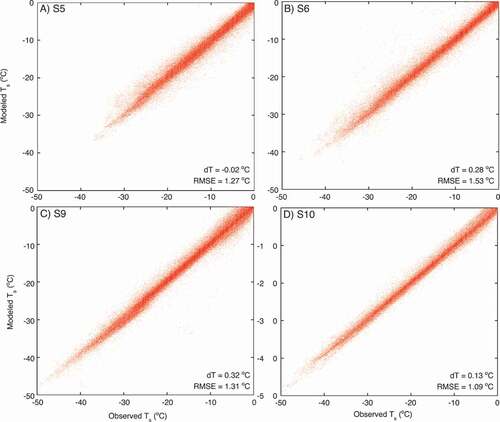
Figure 2 compares modeled and observed values of T_s at the four AWS locations. The mean difference between observations and model values ranges from −0.02 K at S5 to + 0.32 K at S9. The root mean-square error (RMSE) varies from 1.09 K at S10 to 1.53 K at S6 (1.27 K at S5 and 1.31 K at S9).

Figure 2. Modeled versus observed surface temperature (°C, hourly values) for automatic weather station (AWS) locations (A) S5, (B) S6, (C) S9, and (D) S10. Mean bias dT and RMSE given in the lower right corner of each panel

During melt, when the surface temperature is fixed at 273.15 K, we assess model performance by comparing it with the observed ice melt from ablation stakes, assuming an ice density of 910 kg m⁻³ to convert height to mass changes in m w.e. This only works well for S5 and S6, where periods of ice melt can be clearly distinguished from snow melt by means of the sonic height ranger data and albedo observations (low albedo indicates that ice is at the surface). Figure 3A compares modeled and observed cumulative ice melt for these stations. For S6, the time series of modeled ablation is incomplete because of the data gaps in the input data, and modeled cumulative ablation was aligned with the stake data in September 2008, 2010, and 2012.

Figure 3. (A) Cumulative ice ablation in m w.e. for stations S5 and S6. Model data in solid lines (S5 in red, S6 in blue). Annual stake observations in squares (S5) and circles (S6). Note that modeled ablation for S6 was aligned to the stake data in September 2008, 2010, and 2012. (B) Annual ice ablation, model versus stake observations (in m w.e.) for S5 and S6

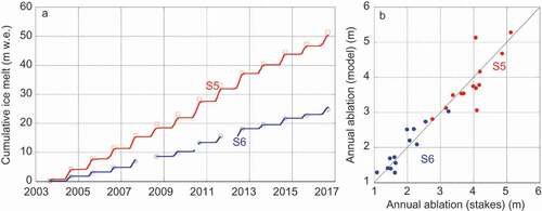
During the thirteen-year period, the total modeled ablation at S5 and S6 amounts to 50.3 and 25.5 m w.e., respectively. At S5 the difference in cumulative ice ablation between the model and the stake observations is +1.1 m w.e.; that is, a relative difference of 2.2 percent. At S6, the modeled cumulative ice ablation is 3.1 percent higher than the stake observations (24.7 m w.e.). Although this is well within the model and measurement uncertainty, the relative differences can be much larger for individual years (Figure 3B). The 2012 melt season at S5 shows significantly larger modeled (5.15 m w.e.) than observed (4.06 m w.e.) ice melt; that is, a 27 percent overestimation. Alternatively, the 2008 melt season at S5 shows significantly smaller modeled ice melt (3.06 m w.e.) compared to the stake observation (4.10 m w.e.) These are the largest discrepancies found in the thirteen-year period. Several explanations are possible, although we have not been able to establish the exact cause for these discrepancies. For instance, the stake measurements may have been unrepresentative for the exact AWS location (these are separated by several meters, and in the hummocky terrain at S5, this can mean significant differences in solar radiation geometry and turbulent fluxes). Model and measurement uncertainties are another source for the discrepancies. Varying input and model parameters of the SEB model within their margins of uncertainty did not resolve the issue. Given that similar errors did not occur at S6, a possible explanation is that Monin-Obukhov similarity in the near-surface layer breaks down at the ice-sheet margin, when air that is heated over the ice-free tundra is advected over the melting ice surface, potentially violating the assumption of horizontal homogeneity. In a similar study, Fausto et al. (2015) found that SEB calculations underestimated the 2012 point melt at a PROMICE AWS site in south Greenland by 17 percent. Apparently, the assumptions used in the SEB model during periods of exceptional melt are not always valid, depending on the meteorological conditions.

Results and discussion

Turbulent fluxes in the lower ablation zone

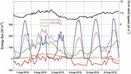
Figure 4 presents time series of monthly mean SEB components at the four AWS sites. In all figures, results for G are excluded because they are small compared to the other fluxes. The high monthly mean values of up to 100 W m⁻² of H at S5 are especially remarkable; this is probably caused by the advection of warm tundra air over the protruding glacier tongues, resulting in very large ice-to-air temperature gradients. In combination with a high surface roughness, this leads to large air-to-ice transport of turbulent sensible heat. The role of turbulent fluxes is illustrated in Figure 5, which shows SEB fluxes and wind speed for a typical six-day summer period. At S5, all SEB components, with the exception of G, show positive peaks in summer, including L and LW_net. The nearly continuous melting ice surface in summer is responsible for this, as shown in Figure 5: it limits the energy loss through LW_out and enables positive surface-to-air temperature and moisture gradients, resulting in downward-directed H and L, further enhancing melt energy. This results in extremely peaked summer melt energy. In the example of Figure 5, increased wind speed on August 2–3 led to significant downward fluxes of H and L, even exceeding SW_net. Integrated throughout the summer (Figure 4), H more than compensates for losses from LW_net, so melt energy at S5 significantly exceeds SW_net during all years, driven by windy and overcast episodes, as shown in Figure 5. The warm summers of 2003, 2007, and 2011–2012 clearly stand out, with July monthly mean melt energies close to or in excess of 200 W m⁻², a value that represents 1.7 m of ice melt during a single month. Together with observations from the southernmost part of Greenland (Fausto et al. 2015), these are among the highest melt energies observed on the ice sheet.

Figure 4. Monthly mean fluxes of net shortwave radiation (blue), net longwave radiation (red), sensible heat (orange), latent heat (green), ground heat (black), and melt (pink). From top to bottom: S5, S6, S9, and S10. The vertical axes are all at the same scale

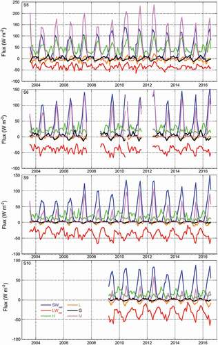
Figure 5. Hourly values of surface energy balance (SEB) fluxes (left vertical axis) and horizontal wind speed (right vertical axis) at S5 during a six-day period in August 2010

Higher up the ice sheet at S9 and S10, a regime of intermittent melt is found, in which in summer the surface usually refreezes during the night. In the beginning and toward the end of summer, some days do not experience daytime melt either. As long as the surface is not continuously at the melting point (i.e., in early summer at S6 and S9 and for most of the summer at S10) increased absorption at the surface of SW_net results in enhanced T_s so that LW_out peaks, and hence LW_net is most negative in summer. In combination with smaller surface-to-air temperature and moisture gradients, summertime H is decreased relative to S5 and L is reversed, leading to net summertime sublimation (negative L) and associated surface cooling.

Drivers of melt and melt variability

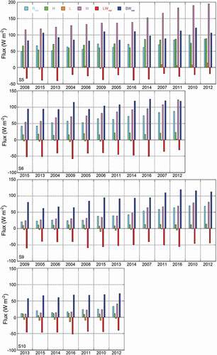
Figure 6 shows June, July, August (JJA)-averaged values of SEB components, sorted by the mean JJA melt flux. This provides useful insight into the drivers of melt at the different locations. At all stations, melt energy peaked in 2012. At S6, S9, and S10 there is correlation of 0.78–0.88 between years with high melt and large SW_net (Table 3). For S5, this correlation is lower at 0.57. The correlation with net radiation (R_net) is high at all stations, from 0.86 at S5 to 0.98 at S6 and S9. This can be ascribed to the fact that the summer surface at these stations consists of firn, enhancing the importance of the snow albedo-melt feedback; that is, the albedo of snow/firn decreases under melting conditions. This effect becomes less important in the ablation zone, where the surface consists of bare ice for most of the melt season: albedo changes are relatively modest and are driven mainly by variations in impurities and algae. At S5, S6, and S9, H plays an important modulating role in the total melt, with a high correlation with JJA melt flux (0.71–0.78, see Table 4). At S5, L is strongly correlated with M (R = 0.88): in high-melt years, there is net deposition, whereas sublimation occurs in years with low melt. In this way, L modulates M by up to 20 W m⁻², averaged throughout summer. The correlation between M and L strongly decreases further inland.

Table 3. Correlation coefficients (R) between June, July, August (JJA) mean melt flux and other surface energy balance (SEB) components

Correlation Coefficient with M	S5	S6	S9	S10
SWnet	0.57	0.78	0.88	0.79
LWnet	0.58	0.66	0.59	0.70
Rnet	0.86	0.98	0.98	0.93
H	0.78	0.74	0.71	0.29
L	0.88	0.78	0.60	0.46

Table 4. Trends in surface energy budget components, expressed in W m⁻² y⁻¹, determined for the period 2003–2016. Trends significant at the p < 0.10 level are shown in bold

Flux Trend (W m^−2 y^−1)		Hydrol. Year			JJA
	S5	S6	S9	S5	S6	S9
SWin	1.2	−0.1	0.8	3.8	0.5	2.4
SWout	0.4	−0.3	−0.6	1.7	−0.6	−1.3
SWnet	0.8	0.2	1.4	2.1	1.1	3.7
LWin	−1.1	−0.8	−0.6	−1.5	−1.0	−1.1
LWout	−0.7	−0.5	−0.1	−0.1	−0.2	0.0
LWnet	−0.4	−0.3	−0.5	−1.4	−0.9	−1.2
Rnet	0.4	−0.1	1.0	0.7	0.2	2.5
H	0.0	0.1	−0.1	0.1	0.1	0.0
L	−0.1	0.1	−0.2	−0.1	0.2	−0.2
M	0.0	−0.1	0.6	0.7	0.3	2.2

Figure 6. Energy fluxes (W m⁻²) averaged over June, July, August (JJA), sorted by JJA-mean melt flux. Years on horizontal axes

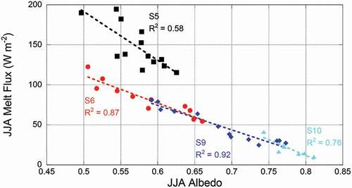
Figure 7 shows the relationship between average JJA albedo and melt energy, underlining the increasing importance of surface albedo variability as a predictor for melt higher on the ice sheet. At S6 and S9, approximately 90 percent of interannual JJA cumulative melt energy variability is explained by variations in albedo. At S5, this is less than 60 percent, indicating the increased role of H and L in explaining interannual variability in melt. At S10, the explained variability is less than at S9 and is only 76 percent. This is in part because of the limited range of albedo observed at this location. The magnitude of the melt dependency on albedo (the slope of the correlation) increases toward the margin, indicating that albedo in the ablation zone is also an indicator for the length of the melt season; that is, long melt seasons are characterized by bare ice being persistently exposed at the surface, decreasing average annual and summer albedo.

Figure 7. Mean June, July, August (JJA) albedo as a function of mean JJA melt flux (in W m⁻²). R² denotes the correlation coefficient

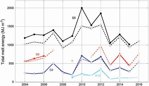
Figure 8 shows the total melt energy during JJA (dashed lines) and during the entire calendar year (January–December, solid lines). At the higher stations, virtually all melt occurs in JJA, and interannual melt energy is determined by these months with the largest solar elevation. This is markedly different at S5, where on average 15–20 percent of the total melt energy derives from outside these three summer months. In high-melt years, this fraction can increase to more than 30 percent. Because these melt events take place at low solar elevation, they are not only driven by radiation but also in part by nonradiative energy fluxes, stressing the importance of sensible heat exchange in particular, in driving extreme melt years. The fact that in the high-melt years (2010 and 2012) also at S9 and S10 a small fraction of melt energy derives from outside of the summer season, indicates that these nonsummer melt events will affect larger parts of the ice sheet when the climate continues to warm and the melt season lengthens.

Figure 8. Total melt energy for each automatic weather stations (AWS) location, in MJ m⁻². June, July, August (JJA) totals in dashed lines with open circles. Annual totals in solid lines with closed circles. S5 in black, S6 in red, S9 in blue, and S10 in light blue

Trends in surface energy balance components

Table 4 shows the trends of all SEB components (calculated both for the hydrological year [September 1–August 31] and for JJA mean, and expressed in W m⁻² y⁻¹) during the period 2003–2016 for stations S5, S6, and S9. We did not include the trends for S10, because the observational period of that station is only five years, too short to calculate meaningful trends. No unequivocal picture emerges from the trend analysis, but some interesting features emerge at all locations. At stations S5, S6, and S9, there is a negative trend in LW_in and LW_net, both for hydrological years and for JJA averages. For the summer (JJA), the trend in LW_net is from −1.2 to −1.4 W m⁻² y⁻¹, significant at p < 0.10 for S5 and S9. At S6, the trend is only fractionally smaller but not significant at that level. For JJA, these negative trends in LW_net can be ascribed mainly to negative trends in LW_in, as the trend in LW_out is near zero at all stations. At all stations, the JJA trends in SW_in and SW_net are positive, and in the case of S5 and S9 they are significant at the p < 0.10 level. Both the decrease in LW_in and the increase in SW_in, in line with satellite and model trends over the Greenland ablation area (Box et al. 2012), suggest a decrease in cloud cover during this period. At S5, JJA SW_out increases because of a decrease in albedo, partially offsetting the increase in SW_in. At S9, however, the JJA SW budget is further enhanced by a reduction in albedo, leading to a negative trend in SW_out. At S6, trends in SW components are much smaller, and are not statistically significant at the p < 0.10 level.

All stations show a positive trend in JJA melt (M), none of which is statistically significant at p < 0.10. At S5 and S9, the increase in M is fully accounted for by the increase in net radiation R_net. No significant trends are found in H. Trends in L are variable and very small, but are statistically significant (p < 0.10) for hydrological years at S6 and S9.

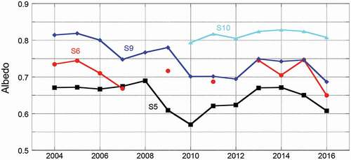
Figure 9 shows trends in SMB-year albedo (an SMB-year or hydrological year runs from September 1 to August 31). A downward trend in albedo is especially conspicuous at S9 (−0.0087 y⁻¹, R = 0.74), close to the equilibrium line. At this location, bare ice was not exposed in summer until 2016, so that snow metamorphosis driven by increased melt has the most pronounced effect on surface albedo. A decreasing albedo at S9 is in line with the upward and inland migration of the ELA (Smeets et al. 2018), and associated meltwater features such as supraglacial lakes (Howat et al. 2013), densification (Machguth et al. 2016; De La Peña et al. 2015), and warming of firn due to meltwater refreezing (Humphrey, Harper, and Pfeffer 2012). A weaker decline is also visible at S5 (−0.0033 y⁻¹, R = 0.36), expressing the lengthening of the melt season. Data gaps prevent a meaningful regression at S6 and S10. The apparent increase at the latter station (+0.0029 y⁻¹) is caused by the start of the time series in the high melt year 2010, where high melt years have a relatively low albedo in the lower accumulation zone.

Figure 9. Albedo, computed from the mean incoming and reflected shortwave fluxes of each mass balance year (September 1, Y-1, to August 31, Y, where the year Y is given on the horizontal axis)

Conclusions

We present a seven- to thirteen-year time series of surface energy balance components, including melt, for four automatic weather stations along the K-transect in west Greenland. In combination with the large natural interannual variability of the Greenland climate, these time series are still too short to derive robust trends from them. However, the stations with the longest record (S5 in the lower ablation zone and S9 around the equilibrium-line altitude) show an increase in SW_net and a decrease in LW_in, highlighting the effect of decreased cloud cover on the increased melt observed at these stations. Further, albedo decrease is strongest at S9, in line with the observations that the ELA is shifting upward, along with other meltwater-related features such as supraglacial lakes and impermeable firn.

These data are indispensable to validate remotely sensed surface characteristics, such as albedo, and to evaluate Greenland climate models. The hourly, daily, and monthly surface energy balance components derived from these stations also greatly improve our understanding of ice-climate interactions over the ice sheet. For instance, the data clearly show that albedo variations explain most of the interannual melt variability at the higher stations, while sensible heat becomes a major heat source for melt in the lower ablation zone. This shift in contribution to melt energy is expected to become more important in a future warmer climate.

Acknowledgments

We thank numerous people for help in the field and for construction and maintenance of the automatic weather stations. Feedback from two reviewers and the editor helped to improve and clarify this manuscript, and their efforts are kindly acknowledged.

Disclosure statement

The authors report no conflicts of interest. The authors alone are responsible for the content and writing of the article.

Additional information

Funding

We acknowledge funding from many sources, the most important ones being NWO (Netherlands Institute for Scientific Research), its Netherlands Polar Programme (NPP), NWO-Spinoza programme, NESSC (Netherlands Earth System Science Centre), and KNAW (Royal Netherlands Academy of Sciences).

References

- Andreas, E. L. 1987. A theory for the scalar roughness and the scalar transfer coefficients over snow and sea ice. Boundary-Layer Meteorology 38:159–84. doi:https://doi.org/10.1007/BF00121562.
- Box, J. E., X. Fettweis, J. C. Stroeve, M. Tedesco, D. K. Hall, and K. Steffen. 2012. Greenland ice sheet albedo feedback: Thermodynamics and atmospheric drivers. The Cryosphere 6:821–39. doi:https://doi.org/10.5194/tc-6-821-2012.
- Charalampidis, C., D. van As, J. E. Box, M. R. van den Broeke, W. T. Colgan, S. H. Doyle, A. L. Hubbard, M. MacFerrin, H. Machguth, and C. J. P. P. Smeets. 2015. Changing surface-atmosphere energy exchange and refreezing capacity of the lower accumulation area, West Greenland. The Cryosphere 9:2163–81. doi:https://doi.org/10.5194/tc-9-2163-2015.
- Cullather, R. I., S. M. J. Nowicki, B. Zhao, and M. J. Suarez. 2014. Evaluation of the surface representation of the Greenland ice sheet in a general circulation model. Journal of Climate 27:4835–56. doi:https://doi.org/10.1175/JCLI-D-13-00635.1.
- Cullen, N. J., T. Mölg, J. Conway, and K. Steffen. 2014. Assessing the role of sublimation in the dry snow zone of the Greenland ice sheet in a warming world. Journal of Geophysical Research 119:6563–77. doi:https://doi.org/10.1002/2014JD021557.
- Das, S. B., R. B. Alley, D. B. Reusch, and C. A. Shuman. 2001. Temperature variability at Siple Dome, West Antarctica, derived from ECMWF re-analyses, SSM/I and SMMR brightness temperatures and AWS records. Annals of Glaciology 34:106–12. doi:https://doi.org/10.3189/172756402781817699.
- De La Peña, S., I. M. Howat, P. W. Nienow, M. R. van den Broeke, E. Mosley-Thompson, S. F. Price, D. Mair, B. Noël, and A. J. Sole. 2015. Changes in the firn structure of the western Greenland Ice Sheet caused by recent warming. Cryosphere 9:1203–11. doi:https://doi.org/10.5194/tc-9-1203-2015.
- Denby, B., and W. Greuell. 2000. The use of bulk and profile methods for determining surface heat fluxes in the presence of glacier winds. Journal of Glaciology 46:445–52. doi:https://doi.org/10.3189/172756500781833124.
- Enderlin, E. M., I. M. Howat, S. Jeong, M.-J. Noh, J. H. van Angelen, and M. R. van den Broeke. 2014. An improved mass budget for the Greenland ice sheet. Geophysical Research Letters 41:866–72. doi:https://doi.org/10.1002/2013GL059010.
- Fausto, R. S., D. van As, J. E. Box, W. Colgan, P. L. Langen, and R. H. Mottram. 2015. The implication of nonradiative energy fluxes dominating Greenland ice sheet exceptional ablation area surface melt in 2012. Geophysical Research Letters 43:2649–58. doi:https://doi.org/10.1002/2016GL067720.
- Greuell, W., B. Denby, R. S. W. van de Wal, and J. Oerlemans. 2001. Ten years of mass-balance measurements along a transect near Kangerlussuaq, central West Greenland. Journal of Glaciology 47 (156):157–58. doi:https://doi.org/10.3189/172756501781832458.
- Häkkinen, S., D. K. Hall, C. A. Shuman, D. L. Worthen, and N. E. DiGirolamo. 2014. Greenland ice sheet melt from MODIS and associated atmospheric variability. Geophysical Research Letters 41:1600–1607. doi:https://doi.org/10.1002/2013GL059185.
- Hall, D. K., J. C. Comiso, N. E. DiGirolamo, C. A. Shuman, J. E. Box, and L. S. Koenig. 2013. Variability in the surface temperature and melt extent of the Greenland ice sheet from MODIS. Geophysical Research Letters 40:2114–20. doi:https://doi.org/10.1002/grl.50240.
- Hall, D. K., J. C. Comiso, N. E. DiGirolamo, C. A. Shuman, J. R. Key, and L. S. Koenig. 2012. A satellite-derived climate-quality data record of the clear-sky surface temperature of the Greenland ice sheet. Journal of Climate 25:4785–98. doi:https://doi.org/10.1175/JCLI-D-11-00365.1.
- Howat, I. M., S. De La Peña, J. H. van Angelen, J. T. M. Lenaerts, and M. R. van den Broeke. 2013. Expansion of meltwater lakes on the Greenland ice sheet. The Cryosphere 7:201–4. doi:https://doi.org/10.5194/tc-7-201-2013.
- Humphrey, N. F., J. T. Harper, and W. T. Pfeffer. 2012. Thermal tracking of meltwater retention in Greenland’s accumulation area. Journal of Geophysical Research 117:F01010.
- Kuipers Munneke, P., S. R. M. Ligtenberg, B. P. Y. Noël, I. M. Howat, J. E. Box, E. Mosley-Thompson, J. R. McConnell, K. Steffen, J. T. Harper, S. B. Das, et al. 2015. Elevation change of the Greenland ice sheet due to surface mass balance and firn processes, 1960–2013. The Cryosphere Discussions 9:3541–80. doi:https://doi.org/10.5194/tcd-9-3541-2015.
- Kuipers Munneke, P., M. R. van den Broeke, C. H. Reijmer, M. M. Helsen, W. Boot, M. Schneebeli, and K. Steffen. 2009. The role of radiation penetration in the energy budget of the snowpack at Summit, Greenland. The Cryosphere 3:155–65. doi:https://doi.org/10.5194/tc-3-155-2009.
- Machguth, H., M. MacFerrin, D. van As, J. E. Box, C. Charalampidis, W. Colgan, R. S. Fausto, H. A. J. Meijer, E. Mosley-Thompson, and R. S. W. van de Wal. 2016. Greenland meltwater storage in firn limited by near-surface ice formation. Natural Climate Change 6:390–93. doi:https://doi.org/10.1038/nclimate2899.
- Nghiem, S. V., D. K. Hall, T. L. Mote, M. Tedesco, M. R. Albert, K. Keegan, C. A. Shuman, N. E. DiGirolamo, and G. Neumann. 2012. The extreme melt across the Greenland ice sheet in 2012. Geophysical Research Letters 39:L20502. doi:https://doi.org/10.1029/2012GL053611.
- Niwano, M., T. Aoki, S. Matoba, S. Yamaguchi, T. Tanikawa, K. Kuchiki, and H. Motoyama. 2015. Numerical simulation of extreme snowmelt observed at the SIGMA-A site, northwest Greenland, during summer 2012. The Cryosphere 9:971–88. doi:https://doi.org/10.5194/tc-9-971-2015.
- Noël, B., W. J. van de Berg, E. van Meijgaard, P. Kuipers Munneke, R. S. W. van de Wal, and M. R. van den Broeke. 2015. Summer snowfall on the Greenland Ice Sheet: A study with the updated regional climate model RACMO2.3. The Cryosphere Discussions 9:1177–208. doi:https://doi.org/10.5194/tcd-9-1177-2015.
- Oerlemans, J., and H. F. Vugts. 1993. A meteorological experiment in the melting zone of the Greenland ice sheet. Bulletin of the American Meteorological Society 74:355–65. doi:https://doi.org/10.1175/1520-0477(1993)074<0355:AMEITM>2.0.CO;2.
- Shuman, C. A., D. K. Hall, N. E. DiGirolamo, T. K. Mefford, and M. J. Schnaubelt. 2014. Comparison of near-surface air temperatures and MODIS ice-surface temperatures at Summit, Greenland (2008–13). Journal of Applied Meteorology and Climatology 53:2171–80. doi:https://doi.org/10.1175/JAMC-D-14-0023.1.
- Smeets, C. J. P. P., P. Kuipers Munneke, M. R. van den Broeke, W. Boot, J. Oerlemans, H. Snellen, C. H. Reijmer, R. S. W. van de Wal, and D. van As. 2018. The K-transect in west Greenland: automatic weather station data (1993–2016). Arctic, Antarctic, and Alpine 50 (1):S100002.
- Smeets, C. J. P. P., and M. R. van den Broeke. 2008. The parameterisation of scalar transfer over rough ice. Boundary-Layer Meteorology 128:339–55. doi:https://doi.org/10.1007/s10546-008-9292-z.
- Steffen, K., and J. E. Box. 2001. Surface climatology of the Greenland ice sheet: Greenland Climate Network 1995–1999. Journal of Geophysical Research 106:33951–64. doi:https://doi.org/10.1029/2001JD900161.
- Stroeve, J. C., J. E. Box, C. Fowler, T. Haran, and J. Key. 2001. Intercomparison between in situ and AVHRR polar pathfinder-derived surface albedo over Greenland. Remote Sensing of Environment 75:360–74. doi:https://doi.org/10.1016/S0034-4257(00)00179-6.
- van As, D., R. S. Fausto, and PROMICE Project Team. 2011. Programme for Monitoring of the Greenland Ice Sheet (PROMICE): First temperature and ablation records. Geological Survey of Denmark and Greenland (GEUS) Bulletin 23:73–76.
- van de Wal, R. S. W., W. Boot, C. J. P. P. Smeets, H. Snellen, M. R. van den Broeke, and J. Oerlemans. 2012. Twenty-one years of mass balance observations along the K-transect, West Greenland. Earth System Science Data 4:31–35. doi:https://doi.org/10.5194/essd-4-31-2012.
- van de Wal, R. S. W., W. Boot, M. R. van den Broeke, C. J. P. P. Smeets, C. H. Reijmer, J. J. A. Donker, and J. Oerlemans. 2008. Large and rapid melt-induced velocity changes in the ablation zone of the Greenland ice sheet. Science 321:111–13. doi:https://doi.org/10.1126/science.1158540.
- van de Wal, R. S. W., W. Greuell, M. R. van den Broeke, and J. Oerlemans. 2005. Surface mass-balance observations and automatic weather station data along a transect near Kangerlussuaq, West Greenland. Annals of Glaciology 41:131–39.
- van de Wal, R. S. W., and J. Oerlemans. 1994. An energy balance model for the Greenland ice sheet. Global and Planetary Change 9:115–31. doi:https://doi.org/10.1016/0921-8181(94)90011-6.
- van de Wal, R. S. W., C. J. P. P. Smeets, W. Boot, M. Stoffelen, R. van Kampen, S. H. Doyle, F. Wilhelms, M. R. van den Broeke, C. H. Reijmer, J. Oerlemans, et al. 2015. Self-regulation of ice flow varies across the ablation area in south-west Greenland. The Cryosphere 9:603–11. doi:https://doi.org/10.5194/tc-9-603-2015.
- van den Broeke, M. R., C. J. P. P. Smeets, J. Ettema, C. van der Veen, R. S. W. van de Wal, and J. Oerlemans. 2008. Partitioning of energy and meltwater fluxes in the ablation zone of the west Greenland ice sheet. The Cryosphere 2:179–89. doi:https://doi.org/10.5194/tc-2-179-2008.
- van den Broeke, M. R., C. J. P. P. Smeets, and R. S. W. van de Wal. 2011. The seasonal cycle and interannual variability of surface energy balance and melt in the ablation zone of the west Greenland ice sheet. The Cryosphere 5:377–90. doi:https://doi.org/10.5194/tc-5-377-2011.
- van den Broeke, M. R., D. van As, C. H. Reijmer, and R. S. W. van de Wal. 2004. Assessing and improving the quality of unattended radiation observations in Antarctica. Journal of Atmospheric and Oceanic Technology 21:1417–31. doi:https://doi.org/10.1175/1520-0426(2004)021<1417:AAITQO>2.0.CO;2.
- van den Broeke, M. R., D. van As, C. H. Reijmer, and R. S. W. van de Wal. 2005. Sensible heat exchange at the Antarctic snow surface: A study with automatic weather stations. International Journal of Climatology 25:1080–101. doi:https://doi.org/10.1002/joc.1152.
- Wientjes, I. G. M., and J. Oerlemans. 2010. An explanation for the dark region in the western melt zone of the Greenland ice sheet. The Cryosphere 4:261–68. doi:https://doi.org/10.5194/tc-4-261-2010.
- Wientjes, I. G. M., R. S. W. van de Wal, G.-J. Reichart, A. Sluijs, and J. Oerlemans. 2011. Dust from the dark region in the western ablation zone of the Greenland ice sheet. The Cryosphere 5:589–601. doi:https://doi.org/10.5194/tc-5-589-2011.