The K-transect in west Greenland: Automatic weather station data (1993–2016)

ABSTRACT

We present twenty-three years (1993–2016) of automatic weather station (AWS) data, collected along the K-transect near Kangerlussuaq in west Greenland. The transect runs from east to west, roughly perpendicular to the ice sheet edge at about 67° N. The K-transect originated from the Greenland Ice Margin Experiments (GIMEX), held in the summers of 1990 and 1991. Until recently, surface mass balance and ice velocity measurements were performed at nine locations along the K-transect, of which four are equipped with AWS: two in the ablation zone at approximately 500 m and 1,000 m asl, one at the approximate equilibrium-line altitude (~1,500 m asl), and one in the lower accumulation zone (~1,850 m asl) at distances of 5, 38, 88, and 140 km from the ice edge, respectively. Here, we present an overview of the various AWS types and their data corrections, quality, and availability, including a preliminary trend analysis. Recent increases in temperature and radiation components are associated with the frequent occurrence of anti-cyclonic conditions in west Greenland, resulting in clear skies and relatively warm summers. Strong melt concurs with a decrease in winter accumulation, lowering the surface albedo of the ice sheet. The AWS situated at 1,500 m asl, the former equilibrium-line altitude (ELA), observed almost a doubling of the summertime net shortwave radiation since 2004; as a result, the ELA along the K-transect has been steadily increasing and is currently situated well above 1,700 m asl.

KEYWORDS:

• K-transect
• Greenland
• automatic weather station

Introduction

Observations unambiguously show that the rate at which the Greenland Ice Sheet (GrIS) loses mass has increased since 1990 (Alley et al. 2005; Rignot and Kanagaratnam 2006; Rignot et al. 2011; Velicogna and Wahr 2006). More than half of this mass loss is caused by an increase in meltwater runoff (Enderlin et al. 2014; van den Broeke et al. 2009a, 2016), following significant atmospheric warming over Greenland (Box and Cohen 2006; Fettweis et al. 2013; Hanna et al. 2008; McLeod and Mote 2015; Tedesco et al. 2016). The surface energy balance (SEB), which determines melt, must therefore be modeled correctly for projections of future GrIS mass loss to be accurate. Doing this for the full GrIS requires the use of a regional atmospheric climate model that resolves the ice sheet climate and SEB at sufficiently high spatial resolution (van de Wal and Oerlemans 1994; Ettema et al. 2009; Fettweis et al. 2010; Gorter et al. 2014; Noël et al. 2016). In turn, these models must be evaluated using in situ climate and SEB observations from the ice sheet surface (Ettema et al. 2010a, 2010b; Noël et al. 2015). These observations are scarce: the operation of automatic weather stations (AWS) in the GrIS ablation zone is difficult, owing to the presence of crevasses, slush, large ice hummocks, and meltwater streams/lakes. To date, this strongly limits the availability of long-term, reliable climate and SEB time series from the GrIS.

This article presents twenty-three years (August 1993–August 2016) of observations from four AWS along the K-transect near Kangerlussuaq, west Greenland, installed and operated by the Institute for Marine and Atmospheric Research of Utrecht University (UU/IMAU; van de Wal et al. 2005, 2012). Throughout the years, AWS data from the K-transect have been used in many applications; recent examples include radiation and turbulent-driven heat exchange (van den Broeke et al. 2008, 2009), variability of the ablation zone surface roughness (Smeets and van den Broeke 2008), melt energy partitioning (van den Broeke, Smeets, and van de Wal 2011), and regional climate model evaluation (Ettema et al. 2010a, 2010b; Noël et al. 2016). Tedesco et al. (2011) and Alexander et al. (2014) used K-transect radiation data to assess GrIS albedo variability in conjunction with remote sensing data. In van de Wal et al. (2008) and van de Wal et al. (2015) shelf-ice velocity variations were related to meltwater production.

This article starts with a short history of the K-transect, including a brief overview of earlier efforts to collect meteorological data on the GrIS. Then we present the different types of AWS that were developed at UU/IMAU and subsequently deployed along the K-transect. We discuss AWS data biases, corrections, and availability for the period under consideration. We study in a preliminary fashion climate trends and discuss these in the context of recent scientific research. The companion article by Munneke et al. (2017) presents SEB components at K-transect AWS sites since 2003, including melt energy, and evaluates how these have evolved over time.

A brief history of AWS measurements along the K-transect

The earliest systematic temperature measurements in Greenland started as early as 1784 in Nuuk (Östergaard, 1856). The founding of the Danish Meteorological Institute (DMI) in late 1872 marks the beginning of official Greenland instrumental records (Box 2002). The first scientific expedition to carry out year-round meteorological measurements in Greenland was performed by Hermann Stade (July 1892–July 1893) at Qarajaq nunatak at the head of Itivdliarssuk Fjord near the settlement of Uummannaq, northern west Greenland, during an expedition led by Erich Dagobert von Drygalski (Mills 2003). The first modern expeditions taking place at the GrIS with a meteorological component were carried out between 1906 and 1931 by Alfred Wegener, and geographically focused on Eismitte at an elevation of 2,900 m. During the period 1949–1953, French expeditions led by Paul-Èmile Victor led to the foundation of EGIG (Expédition Glaciologique Internationale au Groenland). From 1957 to 1974, further climatological exploration of the GrIS took place along the central EGIG line (e.g., Ambach 1977a, 1977b). It was not before 1990 that similarly extensive meteorological observations were again performed on the GrIS. In that year, two meteorological observations were simultaneously performed in west Greenland by the ETH (Eidgenössische Technische Hochschule) Zürich and the UU/IMAU (Institute for Marine and Atmospheric research Utrecht, Utrecht University).

The ETH carried out experiments at Swiss Camp, situated near the equilibrium line 89 km east of Illulisat (Jacobshavn) and 20 km south of the EGIG profile (Greuell and Konzelmann 1994). About 300 km further south, UU/IMAU executed the Greenland Ice Margin Experiment (GIMEX), with ten measurement locations along a transect running from the tundra in front of Russell Glacier near Kangerlussuaq (west Greenland) to the equilibrium line at an elevation of approximately 1,500 m asl (Oerlemans and Vugts 1993; van den Broeke, Duynkerke, and Oerlemans 1994; van de Wal and Russell 1994). Both experimental efforts evolved into a network of surface mass balance (SMB) and AWS observations: Swiss Camp became part of the Greenland Climate Network (GC-net; Steffen and Box 2001), and GIMEX became home of the K-transect. GC-net was established in 1995 as a part of the Program for Arctic Regional Climate Assessment (PARCA), a NASA initiative, and currently consists of approximately eighteen AWS distributed across the GrIS along the ice-sheet crest (4), the 2,000 m elevation contour (10), and in the ablation area between Swiss Camp and the ice edge (4) (http://cires.colorado.edu/science/groups/steffen/gcnet/). Since 2007, a third network of AWS was established under the Program for Monitoring the Greenland Ice Sheet (PROMICE; http://www.promice.org), launched by the Danish Energy Agency (DANCEA). The network is operated by the Geological Survey of Denmark and Greenland (GEUS) in collaboration with the Danish Technical University (DTU) and the Greenland Survey (Asiaq). Between 2008 and 2010, twenty-three PROMICE AWS were installed in the ablation area and one in the accumulation area.

The GIMEX expeditions in the summers of 1990 and 1991 were the first attempts to study the spatial variability of the summertime climate and the SEB of the GrIS ablation zone (Oerlemans and Vugts 1993). In 1991, in collaboration with the Free University of Amsterdam (FUA), UU/IMAU installed three AWS in the tundra and eight stations on the ice, ranging from the low ablation area at approxmately 300 m asl (S4) to the equilibrium line at 1,520 m asl (S9). AWS were operated at three ice sites (S4, S5, and S6), and site S9 was equipped with a 30 m-high meteorological tower, as well as surface-based remote sensing instruments (SODAR, RASS) to measure wind and temperature profiles. Just in front of the ice edge, a tethered balloon was operated. Figure 1 summarizes the measurements performed along the K-transect during GIMEX-91.

Figure 1. Overview of the GIMEX91 experiment. AWS and SMB stakes were placed along an east–west running transect roughly perpendicular to the ice-sheet edge along the 67 N latitude line. UU/IMAU had a camp close to the ice edge (location 3, tethered balloon), while de FUA camp and boundary layer station, including a 31 m tower, were situated on the ice sheet (location S9). Location S10 was first established as an SMB site in August 1994. Blue represents the current SMB/GPS stations and red the current AWS sites

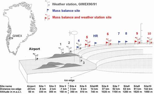
Ever since the first GIMEX experiment in 1990, UU/IMAU has returned to the K-transect at the end of summer (late August, early September) to perform SMB (stake) and ice-velocity (GPS) measurements at eight locations. Currently covering twenty-six years (1990–2016), this is now the longest continuous SMB time series along a transect in Greenland (Machguth et al. 2016b; van de Wal et al. 2012). To improve the interpretation of the yearly SMB measurements, in August 1993 UU/IMAU installed the first K-transect AWS (Type I, Figure 3A and 3C) as well as automated surface height measurements in the lower ablation area at location S5 (~500 m asl, 5 km from the ice edge). In August 1995, another Type I AWS was installed at location S6 (~1,000 m asl and 38 km from the ice edge), followed in August 2001 by a third AWS of this type near the equilibrium line (S9, ~1,500 m asl, 88 km from the ice edge). In August 2003, all three AWS were replaced by Type II AWS (Figure 3B and 3D).

To complement the SMB and AWS measurements, robust single-frequency GPS receivers, designed to be easily fixed to an ablation stake, were added to all eight locations along the K-transect in August 2007 (Den Ouden et al. 2010). As a contribution to GC-net, a fourth Type II AWS was installed in August 2010 in the lower accumulation area at S10 (1,850 m asl, 140 km from the ice edge). This site is especially suitable to monitor percolation processes and a possible upward migration of the equilibrium line. For various reasons (logistics and redundancy) this AWS was again removed in April 2016.

The K-transect field area

The K-transect (Figure 1) is named after the town of Kangerlussuaq, the former U.S. military air base Søndre Strømfjord in west Greenland, just north of the Arctic Circle. In this part of Greenland, the strip of hilly tundra between the ocean and ice sheet is relatively wide (~100 km) and intersected by the approximately 140 km-long fjord Kangerlussuaq. The relatively great distance to the ocean results in a low Arctic and continental climate, with average summer and winter air temperatures of –18.0 and 9.3°C, respectively (climate period 1961–1990, Box 2002), and low annual precipitation (~120 mm w.e. [water equivalent]). The climate is sunny with a monthly mean of 241 sun hours from May to August. The ablation area of the ice sheet starts at the snout of Russell Glacier, 22 km east of Kangerlussuaq at about 350 m asl, and gently slopes inland to meet the equilibrium line 90 km eastward at ±1,553 m asl (period 1991–2011, van de Wal et al. 2012), close to site S9 (1,520 m asl). Table 1 lists average meteorological variables from Kangerlussuaq and all three AWS for the period from August 2003 to August 2016. Moving from S10 toward Kangerlussuaq, most values gradually change in accord with the changing surface elevation, but the wind direction and constancy values clearly distinguish the GrIS from the ice-free tundra. Over the GrIS the wind direction is very constant because of its katabatic origin: both in winter (radiative cooling) as in summer (melting surface) the cold air over the ice flows down its sloping surface. The decrease in wind speed going from S10 to S5 relates to the roughening of the ice surface toward the ice edge, which reduces the wind speed at a constant height (van den Broeke et al. 2009b). While the air flows down its moisture content increases, but at the same time its relative humidity decreases because of the increasing temperature.

Table 1. Climatology at Kangerlussuaq (Kanger) and the AWS locations for the period from August 2003 to August 2016. The wind directional constancy is calculated as the ratio of the magnitudes of the average vector and absolute wind speed

Location	Kanger	S5	S6	S9	S10
Height (m asl)	50	490	1020	1520	1850
Distance from ice edge (km)	22	6	38	88	140
Wind speed u (ms^−1)	3.9	5.3	6.7	7.3	7.2
Temperature T (°C)	−3.9	−5.8	−10.2	−12.7	−15.6
Relative humidity RH (%)	65	77	87	90	92
Specific humidity q (gkg^−1)	2.8	2.4	2.2	2.0	1.8
Wind direction dd (°)	65	115	130	127	128
Directional constancy	0.56	0.89	0.89	0.85	0.68

UU/IMAU AWS Types I and II

The two basic UU/IMAU AWS types that were deployed during the period under consideration are indicated as Type I and Type II (Figure 2). Table 2 lists the make and specifications of sensors, dataloggers, and batteries for both AWS types. The design of Type I (Figure 2A and 2C) was based on the Aanderaa AWS 2700 weather station, with a single sensor T-bar mounted on top of a telescopic mast at about 4 m above the surface. A similar Aanderaa station is currently still commercially available. The telescopic mast was placed on top of a custom-made aluminum cylinder housing the datalogger and batteries. Power is provided by lithium batteries, motivated by the simplicity of the energy system and the excellent specifications of this battery type for temperatures as low as −55°C. Usually about ninety-six batteries were used, which can power a Type I station for about five years. To minimize power consumption, mechanical ventilation for temperature and humidity sensors is not used. Inside the aluminum cylinder at about 0.5 m above the surface air pressure, datalogger temperature and battery voltage are measured.

Table 2. List of instruments used at UU/IMAU AWS Type I and Type II. The periods represent mass balance years, September 1 to August 31

Variable	Sensor type	Period	Accuracy	Sampling interval (minutes)
AWS Type I (1993–2001)
wind speed	Aanderaa 2740	1993–2001	0.5 ms^−1	6
wind direction	Aanderaa 2750	1993–2001	5°	60
temperature	Aanderaa 2775C	1993–2001	0.1°C at −20°C	6
temperature	Vaisala HMP35C	1998–2002	0.2°C	6
humidity	Vaisala HMP35C	1998–2002	2% (RH <90%)	6
radiation shield	Aanderaa made	1993–2001	/	/
radiation shield	Young 41003	1998–2002	/	/
short wave radiation	Aanderaa 2770	1993	10 Wm^−2	6
net radiation	Kipp & Zonen CNR1	1998–2002	daily total ±10%	6
surface/sensor height	height ranger SR50	1993–2002	0.01 m	60
pressure	Aanderaa 2775C	1993–2002	0.5 hPa	60
datalogger	Campbell CR10	1995–2002	/	/
batteries	Tadiran 3.6 V, 35 Ah	1993–2002	/	/
datalogger temperature	Aanderaa	1996–2002	0.1°C	60
battery voltage	Aanderaa	1996–2002	0.1 V	60
AWS Type II (2002–2016)
wind speed	05103-L R.M. Young	2002–2016	0.3 ms^−1	5
wind direction	05103-L R.M. Young	2002–2016	3°	5
temperature	Vaisala HMP45C	2002–2016	0.2°C	5
humidity	Vaisala HMP45C	2002–2016	2% (RH <90%)	5
radiation shield	Young 41003	2002–2016	/
net radiation	Kipp & Zonen CNR1	2002–2016	daily total ±10%	5
surface sensor height	height ranger SR50	2002–2016	0.01 m	30 or 60
pressure	Vaisala PTB101B	2002–2016	0.5 hPa	30 or 60
datalogger	Campbell CR10	2002–2016	/	/
batteries	Tadiran 3.6 V, 35 Ah	2002–2016	/	/
datalogger temperature	Campbell	2002–2016	0.1°C	30 or 60
battery voltage	Campbell	2002–2016	0.1 V	30 or 60

Figure 2. Schematic drawings of UU/IMAU Type I (A) and Type II (B) AWS. (C) Type I AWS (1996), Vatnajökull Ice Cap. (D) Type II AWS (Greenland, 2006 location S5). Note that the sonic height ranger is attached to the AWS in (A) and (B), whereas in the ablation area it is mounted on a separate pole drilled into the ice

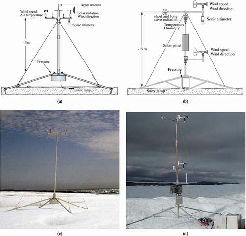
Because of high summer melt rates in the ablation area, the AWS mast cannot be fixed rigidly to the surface. Instead, the mast is supported by four legs that extend outward from the center at a small angle with the surface. Once placed, the legs melt about 0.5 m into the ice where they become firmly fixed. With this design, the AWS sinks downward with the ablating ice surface, ensuring an almost constant measurement height in the course of the ablation season as well as an approximately upright position, typically within a few degrees.

The data storage interval for AWS Type I was one hour; air temperature and radiative fluxes were sampled every six minutes, while for wind speed this is a true average because the pulses from the rotor rotation are counted and averaged once every hour. The surface height, wind direction, pressure, battery voltage, and internal temperature are measured instantaneously at the end of the storage interval. In the ablation zone the sonic altimeters are mounted on a separate pole drilled into the ice surface close to the AWS. In August 1997, the Aanderaa pyranometer was replaced by a net-radiometer (Kipp & Zonen CNR1) that separately measures downwelling and upwelling shortwave and longwave radiation flux components, as well as the temperature of the instrument body. In August 1998, a second Aanderaa temperature sensor was added, mounted inside a substantially larger but still naturally ventilated radiation shield (Young 41003, see the photograph in Figure 2D). A larger radiation shield reduces the error caused by the combined effect of low wind speed and strong insolation. Since August 2008 the Aanderaa cup anemometer was replaced by a propeller vane wind speed/direction sensor (Young 41003). As with the Aanderaa sensor the number of rotations is counted (three pulses per cycle) so that the output values represent a true average wind speed during the sample interval.

In August 2001, the first Type II AWS (Figure 2B and 2D) was deployed at S6. Compared to Type I, this type uses a different mast and instrumentation, and has two measurement levels for wind speed/direction and temperature/humidity measurements at heights of about 2 m and 5 m (see Figure 2D). The AWS mast is telescopic and fixed to a multipurpose aluminum mast foot manufactured by Letrona AG (Switzerland), with four telescopic legs that can be folded for easier transport and installation. The datalogger and batteries are mounted in separate watertight boxes connected to the mast about 1 m above the ice surface. Atmospheric pressure, battery voltage, and internal temperature are measured inside the datalogger box. The storage interval was thirty minutes (but one hour during the period from August 2004 to August 2006). Samples of the wind direction, air temperature, relative humidity, and radiative fluxes are taken every five minutes and then averaged at the storage interval. At the end of each storage interval the instantaneous values for surface height, pressure, battery voltage, internal datalogger box temperature, and the radiometer tilt angles are stored. Both AWS types can be programmed to transmit data via the ARGOS satellite system (www.argos-system.org/web/en/361-climatology.php), allowing the monitoring of near-live climate data (http://www.projects.science.uu.nl/iceclimate/aws).

Data corrections, availability, and bias

In this section, we discuss the data corrections as supplied by the manufacturer, additional corrections necessary to improve data quality, data-replacement techniques (data gap filling) in case of AWS failure, and inhomogeneities in the time series caused by changing measurement systems, locations, or measurement heights. Finally, an overview of data availability for the period 1993–2016 is presented for each AWS.

Radiation data

From August 1993 to August 1997, shortwave radiation was measured using an Aanderaa pyranometer. After August 1997, all AWS were equipped with Kipp & Zonen CNR1 net radiometers, enabling the separate measurement of incoming and outgoing shortwave (SW) and longwave (LW) radiation fluxes. Calibration coefficients as supplied by the manufacturer are applied to convert raw signals into physical units. Van den Broeke et al. (2004) compared CNR1 measurements to data of the Baseline Surface Radiation Network (BSRN) station Neumayer (Antarctica) and concluded that the sensor performs considerably better than the specifications provided by the manufacturer (i.e., 10% for daily totals). The root mean square differences for daily mean incoming SW and LW radiation were found to be about 2.7 percent, or 4.8 W m⁻², and 1.2 percent, or 2.7 W m⁻², respectively.

On installation of the CNR1 instruments in August 1997 at S5 and S6, the Aanderaa pyrometers were left for one year for comparison. Remarkable and identical response deviations from both Aanderaa instruments were observed: the sensitivity differed about 10 percent, and the incoming SW radiation behaved markedly non-linear, indicating cosine response problems. As mentioned earlier, the quality of the SW radiation sensors from the Kipp & Zonen CNR1 has been demonstrated not only by van den Broeke et al. (2004) but also during other unpublished comparison experiments carried out by the IMAU at the BSRN station at the Cabauw observatory in the Netherlands. We use the period with overlap in data to derive a correction that is applied to all remaining Aanderaa SW_in data.

To save energy, radiation sensors at the K-transect AWS are not heated or ventilated. It is demonstrated by van den Broeke et al. (2004) that the single-domed Kipp & Zonen CM3 SW radiation sensors used in the CNR1 are less susceptible to riming than higher-specification double-domed sensors. In combination with the near-continuous katabatic winds in the ablation zone of the GrIS, icing or riming problems are rare. However, the accuracy of measured incoming SW radiation can be considerably compromised by tilt (van den Broeke et al. 2004; Wang et al. 2016), especially with a free-standing mast placed on a melting ice surface. Unfortunately, we lack a consistent set of tilt data for the complete time series: only from August 2008 onward are hourly tilt measurements available. Before that date, the tilt and heading of the radiometers was manually observed once per year during maintenance visits at the end of August. The variability of the tilt, sometimes several degrees during a melt season, makes it difficult to derive reliable tilt corrections before August 2008. Van den Broeke et al. (2004) suggested that SW_out be used as a basis to calculate more accurate values for SW_net, because it is comprised mainly of diffuse, isotropic radiation and hence much less sensitive to tilt. First, a so-called accumulated albedo (α_acc) is calculated as the ratio of accumulated |SW_out| and SW_in values during a time window of 24 h centered around the moment of observation. Then, α_acc is used to retrieve an estimate for the instantaneous net shortwave radation. The underlying idea is that the surface albedo changes are small at sub-daily timescales, while using α_acc eliminates the errors in SW_in associated with a poor cosine response of the instrument and phase shifts due to tilt. In the future, we aim to apply the more sophisticated Retrospective, Iterative, Geometry-Based (RIGB) method developed by Wang et al. (2016). Based on the geometric relationship between the tilted insolation observations and simulations on a horizontal surface on clear days, the tilt angles and directions are deduced and then used to correct the tilt-induced biases on the neighboring cloudy days.

Longwave radiation measurements are corrected for the internal instrument temperature in order to obtain the true temperature of the object that it is facing. Hence, a factor 5.67 × 10⁻⁸ T_CNR⁴ has to be added to the calibrated sensor output with TCNR1 being the internal CNR1 body temperature in Kelvin. On a few occasions during summer the body temperature sensor produced erroneous readings related to moisture. To substitute these data, we used the correlation that exists between the body temperature of the CNR1 and the temperature measured inside the datalogger box. Both temperature sensors are in an enclosure subject to heating by shortwave radiation and cooling by wind speed; therefore, their response characteristics are comparable. The accuracy of this alternative CNR1 body temperature is estimated to be better than 1°C, resulting in an added uncertainty in the longwave radiation components no larger than 3 W m⁻¹.

Longwave radiation sensors may suffer from the so-called window heating effect, when the window of the LW radiation sensor is heated with respect to the instrument body because of absorbed shortwave radiation, leading to a positively biased longwave radiation measurement (Philipona, Fröhlich, and Betz 1995). For the CG3 LW sensor deployed in the Kipp & Zonen CNR1, this bias can be as large as 10 to 15 W m⁻², depending on the thermal connection between the window and aluminum casing of the instrument. A simple correction for window heating is applied as a function of SW_out, using the 0°C melting ice surface as a reference. A selection of data is based on the assumption that melt occurs at the surface when the air temperature measured by the AWS at 3.5–4.5 m height exceeds 1°C. The upper bound of LW_out values are then fitted to give an instrument-specific offset and sensitivity. To avoid bias owing to the replacement of instruments, we recalculate this correction for each data set obtained between maintenance visits. The correction that is determined for the lower sensor is also applied to the upper sensor, using SW_in to calculate the offset. It should be remembered, however, that we do not know the exact window heating characteristics for the upper sensor. As a result, this correction slightly alters the LW_net values depending in size on the surface albedo.

Temperature data

Air temperature measurements used two different sensors and two different naturally ventilated radiation shields (Table 2). Before August 1998, the Aanderaa temperature sensor was housed in an Aanderaa radiation shield. After August 1998, a second Aanderaa temperature sensor was added in combination with a Young 41003 radiation shield. After August 2001, all Aanderaa temperature sensors were replaced by Vaisala HMP35 temperature/humidity sensors housed in a Young 41003 radiation shield.

Using different sensors and radiation shields may cause an inhomogeneous time series. Systematic differences arising from different sensors are likely to be smaller than the uncertainties from using two different radiation shields: temperature differences between sensors during conditions with considerable wind speed (>6 m s⁻¹) were always well below 0.5°C, while excess temperatures inside naturally ventilated radiation shields during conditions with low wind speed and high insolation can easily exceed 1°C.

The Aanderaa and Young radiation shields both have louvered constructions, but the former is about three times smaller, and the inside of its louvre panels are painted black to prevent internal reflections. However, this also leads to additional heating when solar radiation hits the housing from below; that is, over highly reflective (snow) surfaces. Under low wind-speed conditions, the differences between the two radiation screens appear to vary randomly within the range of 1°C. Part of this randomness is probably caused by the asymmetry in the mounting of sensors with respect to the incident solar radiation. It was decided to correct all temperature data for radiative heating in the same way.

We developed a correction procedure for radiation heating effects based on the model of Jacobs and McNaughton (1994) for overheating of a thermocouple. Similar methods are presented by, for example, Huwald et al. (2009) and Nakamura and Mahrt (2005). As reference, we use radiation-corrected temperature data from a thin wire thermocouple (Campbell FW3 Type E, thickness 0.003 inch) that was installed at site S6 AWS without radiation protection during the period from August 2003 to August 2004. The method is described in detail in the Online Appendix (“Excess Temperatures”). The accuracy of the corrected temperature data is better than 0.5°C for a wind speed greater than 1 m s⁻¹.

Humidity data

Relative humidity (RH) is measured with a Vaisala HMP35 or HMP45 probe equipped with virtually identical temperature (T) and RH sensors since August 1998. There are two sources of error for which we apply an additional correction. The probe is mounted inside a naturally ventilated radiation shield, and for reasons of protection the small T and RH sensors are enclosed inside a small teflon filter at the top of the probe. During conditions with high insolation and low wind speed this naturally heated enclosure leads to a negative bias in the RH measurements. To correct for this, temperature data from the same probe with and without the excess heating correction (see section “Temperature data”) are used to calculate the corresponding saturation pressures from which we can recalculate the RH of the outside air. This procedure is the same as presented by Makkonen and Laakso (2005) for an artificially heated Vaisala probe.

Second, the RH sensor is calibrated with respect to water. This means that RH at subfreezing temperatures is underestimated, because the sensor is in equilibrium with ice that supports a lower saturation pressure. We adopt the rescaling method introduced and tested by Anderson (1994) and referred to by others such as Makkonen and Laakso (2005). First, the raw RH values are converted to those over ice by multiplying with the ratio of the saturation pressures for water and ice. At subfreezing temperatures, the resulting maximum RH values are still usually found to be well below 100 percent, which we call RH_max(T). This is a consequence of the limited validity range of the built-in temperature correction (Anderson 1994). In a second correction step, the maxima of RH_max(T) are estimated by averaging the upper 5 percent of data at subfreezing temperatures in 1°C temperature bins, and assuming these to represent 100 percent RH. Each RH value is then multiplied with 1/RH_max(T), because the error is not an offset but, rather, is associated with the gain of the instrument.

Sonic height ranger data

Surface height changes that result from accumulation/ablation are measured using the Campbell Scientific SR50 sonic height ranger (SHR). This sensor uses sound pulses to measure the distance to the surface. The output signal must be temperature corrected using ${\mathrm{H}}_{\mathrm{c}\mathrm{o}\mathrm{r}\mathrm{r}}={\mathrm{H}}_{\mathrm{r}\mathrm{a}\mathrm{w}}\sqrt{{\mathrm{T}}_{\mathrm{a}\mathrm{i}\mathrm{r}}/273.15}$, with H_corr the corrected distance between the surface and the SR50; H_raw the raw SR50 output signal; and T_air the average temperature of the air layer between sensor and surface. No air temperature data were available for the periods from August 1996 to August 1997 at S5 and August 1995 to August 1996 at S6. For these periods, air temperature is estimated from the sensitivity of the battery voltage to temperature. Battery voltage is sensitive not only to temperature but also to battery power; that is, decreasing battery power increases the temperature sensitivity. Using data from the AWSs at S5 and S6 for the period from August 1996 to August 1997, a quadratic relationship was found, providing an air temperature estimate with a standard error of about 3°C, leading to a maximum additional error for surface height values of about 0.03 m for a height of 5 m.

Wind speed and direction data

Wind speed measurements were performed with two different types of sensors. During 1993–2002, on AWS Type I a cup anemometer (Aanderaa 2740) was used, which in August 2002 was replaced by a propeller-vane anemometer (R.M. Young 05103).

We compared propeller-vane anemometer data with that of a reference instrument, a sonic anemometer (operated between August 2003 and August 2004 at S6, Greenland), and found agreement to within 1 percent. This confirms the linear behavior that is expected from this type of anemometer (Wyngaard 1981). Additional corrections are therefore not applied to the propeller-vane anemometer data.

For the Aanderaa 2740, initially the manufacturers calibration was applied to the raw data. However, cup anemometers are known to suffer from overspeeding in turbulent flow. Desai, Desa, and Vithayathil (1992) found 5 percent overspeeding for an Aanderaa cup anemometer with respect to a R.M. Young propeller-vane anemometer to be valid under moderately turbulent conditions within the slightly stable boundary layer conditions commonly found in the ablation area of the GrIS. The same estimates for overspeeding are reported in the review by Wyngaard (1981). We therefore simply reduce the Aanderaa wind speed values by 5 percent.

Another difference between these two types of anemometers is their threshold value, which can be less than 0.3 m s⁻¹ for a well-maintained cup anemometer, but can be as much as 1 m s⁻¹ for a propeller vane. Hence, for occasions with a wind speed of 1 m s⁻¹ or less the propeller can stop rotating, underestimating the true wind speed. Wind-speed and direction values less than a threshold of 1 m s⁻¹ are, therefore, to be used with caution. Wind-direction data are only corrected for an offset from true north and for the magnetic declination, which is substantial at the K-transect with values ranging from −38° to −30° during the period from 1993 to 2016.

Data availability

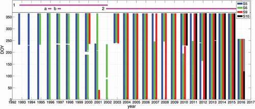
Figure 3 presents an overview of K-transect AWS data availability from August 1993 to August 2016. The horizontal bars at the top of the plot indicate when different types of AWS and/or separate sensors were in use: 1 AWS Type I, 2 AWS Type II, and during periods (A) and (B) only a surface height ranger was present at locations S5 and S6, respectively. K-transect visits usually take place at the end of August, and that is why time series sometimes start around day-of-year (DOY) 250. An especially important date is August 2003, when Type II AWS replaced older stations at locations S5, S6, and S9. AWS data loss is in most cases associated with datalogger-related problems; that is, a failure of the power supply or the collection/writing of data to memory. Individual instruments only rarely fail. Online Appendix Table A1 lists the percentages of available data per year and location, and includes (possible) causes for data gaps in some time series. Note that S10 data gaps (in particular after removal of the station in April 2016) were filled using the PROMICE AWS (KAN, http://www.promice.org) at approximately the same location. Finally, Table 3 summarizes the performance of all AWS, distinguishing for periods with an AWS Type I, Type II, or the complete time series.

Table 3. Overview of available data in percentages per AWS for three different periods

		1993–2002	2003–2016
Period	1993–2016	Type I	Type II
S5	94	85	>99
S6	83	80	85
S9	/	47	>99
S10	/	/	>99

Figure 3. Overview of the available AWS data along the K-transect for the period from August 1993 to August 2016. For every year, all days of the year (DOY) with available data are plotted as colored vertical bars for every AWS. The grey part in 2016 at S10 indicates that for this period PROMICE AWS data are used. Purple horizontal bars indicate what type of AWS was used: 1 AWS Type I, 2 AWS Type II, and during periods (A) and (B) only a surface height ranger was present at locations S5 and S6, respectively

Time series inhomogeneity

The quality of long time series can be compromised by inhomogeneities caused by changes in sensors, sampling, or relocation of AWS necessitated by unfavorable surface conditions (crevasses, lakes, meltwater streams). Changing from AWS Type I to Type II included a change of sensor types, sensor height, sensor housing, and data-sampling strategy, as listed in Table 2. This affected the measurements of temperature, wind speed, wind direction, radiation, and air pressure and was discussed previously.

A change in measurement height causes a bias in the presence of vertical gradients; benchmark sensor heights are measured during the yearly maintenance visits and can be combined with acoustic ranger data to obtain instantaneous sensor heights throughout the year. Sensor height changes are mainly caused by the seasonal snow cover, with typical with typical values between 0.3 m (S5) and 1.0 m (S10). From August 1996 to August 2001 (Type I) the measurement height varied between approximately 3.5 m and 4.5 m. After August 2001, measurement heights for the two-level AWS Type II were about 2 m and 5 m. In order to assess the influence of changing measurement heights, we calculated the vertical gradients for temperature, humidity, and wind speed at S5, S6, and S9 using data after August 2003. All gradients are found to have a seasonal variation and the maximum expected variations for temperature, humidity, and wind speed per meter height variation is about 0.2°C, 1.5 percent, and 0.35 m s⁻¹, respectively. These represent the maximum errors for migration from Type I to Type II.

Differences in the data-sampling strategy between AWS Types I and II (see Table 2) are small for most parameters, and no significant bias is expected. The AWS at S5 was relocated across a distance of 1–2 km (elevation difference 50 m) in August 2003 and August 2008, following deteriorating surface conditions. Possible biases can be expected but are unknown and are not corrected for (see Figure 4 and Figure 6).

Figure 4. Mean JJA values for (A) air temperature, (B) shortwave incoming radiation, (C) albedo, and (D) longwave incoming radiation for AWS S5, S6, S9, and S10. Subplot (A) includes air-temperature data from the DMI meteorological station at Kangerlussuaq airport

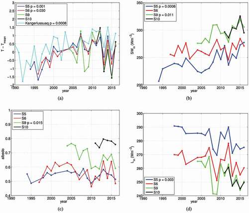
Figure 5. (A) NAO index anomalies relative to the 1981–2010 baseline and averaged each year for summer months (JJA). (B) Normalized values of the mean November–February precipitation and temperature at Kangerlussuaq, the NAO index, and the temperature at S9

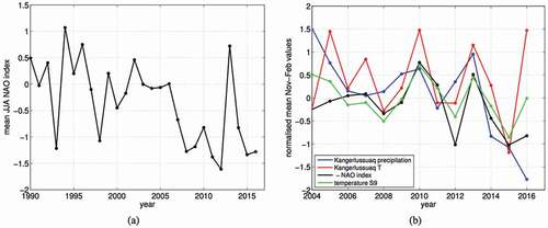
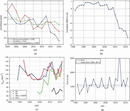
Figure 6. (A) Normalized yearly snow accumulation at S9, winter precipitation at Kangerlussuaq airport, and mean JJA albedo at S9; (B) cumulative SMB (m w.e.) at S9; (C) JJA mean net SW radiation at S5, S6, S9, and S10; (D) Equilibrium Line Latitude (ELA), defined as the altitude where SMB = 0, as estimated from inter/extrapolation of annual SMB profiles (van de Wal et al. 2012)

A case study of changing conditions at S9

AWS data from the K-transect have been used in many studies to characterize the surface-layer climate of the GrIS ablation zone. Examples are the seasonal cycle and interannual variability of the SEB, specifically surface radiation and turbulence fluxes (van den Broeke et al. 2008, 2009b, 2011). Here, based on the homogenized time series of twenty-three years, we analyze some basic aspects of trends in melt across the GrIS. Mote (2007), Hanna et al. (2008), Fettweis (2007), and Fettweis et al. (2011) attributed part of the increase in melt that started in the early 1990s to more frequent anticylonic conditions across the GriS in combination with a warmer background atmosphere. Figure 4 shows trends in June, July, and August (JJA) averages of air temperature, incoming shortwave and longwave radiation, and albedo for all K-transect AWS. We added the time series of air temperature of the Danish Meteorological Institute (DMI) station at Kangerlussuaq airport. In case of a significant trend in a time series we added the corresponding p value. Not all time series are continuous, and it should be noted that the dots represent the measured values. Both the positive trend and interannual variability in mean JJA west Greenland air temperatures since 1992 (post-Pinatubo event), as previously reported in, for example, Hanna et al. (2008), are confirmed at S5, S6, and Kangerlussuaq airport (Figure 4A). The trends for the latter time series are significant, while those for S9 and S10, being much shorter, are not. Since 2005 the temperature trend is insignificant at all locations, owing in part to a succession of cold and warm summers between 2012 and 2016.

Judging from reanalysis-forced SMB reconstructions from regional climate models, recent GrIS melt rates are unprecedented during the past sixty years (van den Broeke et al. 2009a; Fettweis et al. 2011; Tedesco et al. 2011, 2013). Fettweis et al. (2010), Box et al. (2012), and Hanna et al. (2012) point out that general circulation anomalies related to a persistently negative summer phase of the North Atlantic Oscillation (NAO) explain an important part of the recent warming. For instance, Fettweis et al. (2013) state that anticyclonic conditions occurred twice as frequently over Greenland during 2007–2012 compared to the average over the past fifty years. In particular, along the west coast of Greenland, the associated circulation anomaly leads to increased warm air advection, increased downward shortwave radiation, and reduced summer snow accumulation. In turn, this results in reduced albedo values, especially in the area just below the equilibrium line (Box et al. 2012). Figure 5A shows time series of the NAO index averaged for the summer months (JJA) as in Box et al. (2012). The persistently negative values that started in 2007 have continued to date, with the exception of the summer of 2013, which was cold at the K-transect and elsewhere in Greenland (Figure 4A).

No significant temperature trend has been observed along the K-transect since 2007 (Figure 4A). In contrast, incoming shortwave and longwave radiation do show well-defined (opposite) trends (Figure 4B, 4D), suggesting an increased frequency of clear sky conditions as expected during anticyclonic conditions. No trends are expected in the albedo at S5 and S6, being located in the lower ablation zone with mostly ice at the surface during JJA (Figure 4C). The interannual variability in albedo, in particular at S6, correlates with air temperature and probably relates to differences in local surface characteristics, such as the roughness of the ice surface and the distribution of impurities in the ice. S6 is situated in the so-called dark zone, which is known for its high impurity concentration (van de Wal and Oerlemans 1994; Wientjes et al. 2011).

A site of special interest is S9, which at the start of the K-transect in 1990 was situated close to the long-term Equilibrium Line Altitude (ELA) of approximately 1,553 m asl (van de Wal et al. 2012). This area of the ice sheet typically has an interannual variation of surface characteristics that affect albedo. Interannual variability of albedo at S9 is large and correlates significantly to air temperature (Figure 4A and 4C; r = 0.63), but it also has a significant downward trend in accordance with findings by Box et al. (2012), He et al. (2013), and Alexander et al. (2014) for the area close to the ELA. The high albedo values at S9 at the start of the time series are reminiscent of (melting) snow and firn; after the recent extreme melt events in the summers of 2007, 2010, and 2012, for the first time in September 2016 the surface at S9 resembled that of bare ice, with small hummocks and clear signs of recent surface meltwater streams. This means that S9 is now situated in the GrIS ablation zone.

An important factor determining summer melt is winter snow accumulation; the mass of the winter snowpack, in combination with early summer melt rates, determines to a large extent the timing of the surfacing of the dark ice surface and hence summer albedo. Figure 6A shows annual winter snow accumulation at S9 as determined from hourly acoustic height ranger data, combined with the mean JJA albedo at S9. Also included is winter precipitation at Kangerlussuaq airport. The winter snow accumulation data are presented as cumulative values for the period from October to April, and are normalized using the 2004 value. A remarkable and significant decrease is seen, with winter accumulation along the K-transect having decreased by more than 50 percent since 2004. The correlation of the variations between snow accumulation and albedo at S9 is particularly high (r = 0.91), while that between snow accumulation and precipitation in Kangerlussuaq is small (r = 0.30).

Appenzeller et al. (1998), Bromwich et al. (1999), and Mosley-Thompson et al. (2005) showed that the interannual variations in winter precipitation in Greenland have a negative correlation to the NAO index, with highest values in the west-central part of the GrIS. In agreement with these findings Figure 5B demonstrates that in particular for the period from 2007 to 2016 the September–April averaged negative NAO index correlates very well to the precipitation and temperature at Kangerlussuaq airport and the temperature at S9. The decreasing winter accumulation at S9 appears therefore to be closely linked to the wintertime NAO index.

We hypothesize that the strong decrease in winter accumulation in combination with the recent extreme melt summers of 2003, 2007, 2010, and later has eroded the firn layer, leaving dark glacier ice below the winter snow at S9, classifying this site henceforth as ablation zone. Shallow ice-core drilling and radar profile data along the K-transect by Machguth et al. (2016a) in the spring of 2013 confirms that below about 1,680 m asl, no firn layer remains. Close to S10, at 1,850 m asl, they found up to 5 m-thick ice layers, formed after 2010 because of refreezing of melt water. To trace the firn erosion at S9 back in time, Figure 6B shows the time series of cumulative SMB since the start of the observations. Between 1990 and 2009, the long-term cumulative SMB at S9 was close to zero; that is, S9 was situated close to the ELA. In contrast, from 2010 onward, about 4 m w.e. of firn and ice has been removed. It appears as if the summer of 2010 marked a transition year, after which the SMB at S9 remained persistently negative. The time series of mean JJA SW_net (Figure 6C) confirms the step change in 2010, with subsequent values almost equaling those in the lower ablation area at S5 and S6. We conclude that in recent years the ELA has shifted upward, sufficiently so much so that S9 is now situated in the GrIS ablation zone. The time series of ELA, estimated from interpolation/extrapolation of the annual K-transect SMB values (Figure 6D), indirectly supports this through a lower ELA bound since 2010 of approximately 1,500 m asl.

Conclusions

Twenty-three years (1993–2016) of automatic weather atation (AWS) and surface mass balance (SMB) data collected along the K-transect in west Greenland are presented. After data homogenization, which attempts to correct for various sensor errors and the use of different sensors and station types where necessary, we show that the K-transect data give useful information about climate and climate trends in this part of Greenland. In addition to their intrinsic value, which enables us to calculate and close the surface energy balance (SEB; see companion article by Munneke et al. [2017]), the data can be used to evaluate (regional) climate models and to validate satellite data. In a preliminary analysis, we show that a significant negative trend in winter accumulation since 1990 has led to a darkening of the surface around the equilibrium line, where the firn layer has been removed and where at the beginning of the melting season bare ice is now present below the winter snowpack. In combination with the frequent recent occurrence of anticyclonic conditions over southwest Greenland during summer, bringing clear skies and warmer air, this has led to an upward shift in absorbed SW radiation. As a result, site S9, at approximately 1,500 m asl, is now considered to be situated below the Equilibrium Line Altitude (ELA, defined as the altitude where SMB = 0); that is, in the GrIS ablation zone. Although the large interannual variations and the uncertainty associated with the interpolation methods make any trend hard to detect, we postulate that since 1990, the ELA at the K-transect has steadily moved upward and lies currently well above 1,700 m asl.

Acknowledgments

We acknowledge funding from many sources, the most important ones being NWO (Netherlands Institute for Scientific Research), its Netherlands Polar Programme (NPP), NWO-Spinoza programme, NESSC (Netherlands Earth System Science Centre), and KNAW (Royal Netherlands Academy of Sciences). We thank numerous people for help in the field and for the construction and maintenance of the automatic weather stations. Data from the Programme for Monitoring of the Greenland Ice Sheet (PROMICE) were kindly provided by Dirk van As from the Geological Survey of Denmark and Greenland (GEUS). The positive feedback from the editor and two reviewers is kindly acknowledged.

References

- Alexander, P. M., M. Tedesco, X. Fettweis, R. S. W. van de Wal, C. J. P. P. Smeets, and M. R. van den Broeke. 2014. Assessing spatio-temporal variability and trends in modelled and measured Greenland Ice Sheet albedo (2000–2013). The Cryosphere 8:1–16. doi:https://doi.org/10.5194/tc–8–2293–2014.
- Alley, R. B., P. U. Clark, P. Huybrechts, and I. Joughin. 2005. Ice-sheet and sea-level changes. Science 310:456–60. doi:https://doi.org/10.1126/science.1114613.
- Ambach, W. 1977a. Untersuchungen zum energieumsatz in der ablationszone des grönländischen inlandeises, expedition glaciologique interna-tionale au Groenland, vol. 4, 63. Kobenhagen: Bianco Lunos Bogtryyeri A/S.
- Ambach, W. 1977b. Untersuchungen zum energieumsatz in der akkumulationszone des grönländischen inlandeises, expedition glaciologique in-ternationale au Groenland, vol. 4, 44. Kobenhagen: Bianco Lunos Bogtryyeri A/S.
- Anderson, P. S. 1994. A method for rescaling humidity sensors at temperatures well below freezing. Journal Atmos Oceanic Technological 11:1388–91. doi:https://doi.org/10.1175/1520-0426(1994)011<1388:AMFRHS>2.0.CO;2.
- Appenzeller, C., J. Schwander, S. Sommer, and T. Stocker. 1998. The North Atlantic Oscillation and its imprint on precipitation and ice accumulation in Greenland. Geophysical Research Letters 25:1939–42. doi:https://doi.org/10.1029/98GL01227.
- Box, J. 2002. Survey of Greenland instrumental temperature records. International Journal Climate 22:1828–47. doi:joc.852/joc.852.
- Box, J. E., and A. E. Cohen. 2006. Upper-air temperatures around Greenland: 1964–2005. Geophysical Research Letters 33:L12706. doi:https://doi.org/10.1029/2006GL025723.
- Box, J. E., X. Fettweis, J. C. Stroeve, M. Tedesco, D. K. Hall, and K. Steffen. 2012. Greenland ice sheet albedo feedback: Thermodynamics and atmospheric drivers. The Cryosphere 6:821–39. doi:https://doi.org/10.5194/tc-6-821-2012.
- Bromwich, D. H., Q.-S. Chen, Y. Li, and R. I. Cullather. 1999. Precipitation over Greenland and its relation to the North Atlantic Oscillation. Journal of Geophysical Research Atmospheres 104:22 103–22 115. doi:https://doi.org/10.1029/1999JD900373.
- Den Ouden, M., C. Reijmer, V. A. Pohjola, R. van de Wal, J. Oerlemans, and W. Boot. 2010. Stand-alone single-frequency GPS ice velocity observations on Nordenskiöldbreen, Svalbard. The Cryosphere 4:593–604. doi:https://doi.org/10.5194/tc-4-593-2010.
- Desai, R., E. Desa, and G. Vithayathil. 1992. A marine meteorological data acquisition system. In Oceanography of the Indian Ocean, ed. B. Desai, 719–31. Oxford: Uitgevers B. V.
- Enderlin, E. M., I. M. Howat, S. Jeong, M.-J. Noh, J. H. Angelen, and M. R. van den Broeke. 2014. An improved mass budget for the Greenland ice sheet. Geophysical Research Letters 41:866–72. doi: joc.3475 /2013GL059010.
- Ettema, J., M. R. van den Broeke, E. van Meijgaard, and W. J. van de Berg. 2010b. Climate of the Greenland ice sheet using a high-resolution climate model—Part 2: Near-surface climate and energy balance. The Cryosphere 4:529–44. doi:https://doi.org/10.5194/tc–4–529–2010.
- Ettema, J., M. R. van den Broeke, E. van Meijgaard, W. J. van de Berg, J. L. Bamber, J. E. Box, and R. C. Bales. 2009. Higher surface mass balance of the Greenland ice sheet revealed by high-resolution climate modeling. Geophysical Researcher Letters 36:L12501. doi:https://doi.org/10.1029/2009GL038110.
- Ettema, J., M. R. van den Broeke, E. van Meijgaard, van de Berg, J. Ettema, E. van Meijgaard, W. J. van de Berg, J. E. Box, and K. Steffen. 2010a. Climate of the Greenland ice sheet using a high-resolution climate model—Part 1: Evaluation. The Cryosphere 4:511–27. doi:https://doi.org/10.5194/tc–4–511–2010.
- Fettweis, X. 2007. Reconstruction of the 1979–2006 Greenland ice sheet surface mass balance using the regional climate model MAR. The Cryosphere 1:21–40. doi:https://doi.org/10.5194/tc-1-21-2007.
- Fettweis, X., E. Hanna, C. Lang, A. Belleflamme, M. Erpicum, and H. Gallée. 2013. Brief communication “Important role of the mid-tropospheric atmospheric circulation in the recent surface melt increase over the Greenland ice sheet.” The Cryosphere 7:241–48. doi:https://doi.org/10.5194/tc-7-241-2013.
- Fettweis, X., G. Mabille, M. Erpicum, S. Nicolay, and M. R. van den Broeke. 2010. The 1958–2009 Greenland ice sheet surface melt and the mid-tropospheric atmospheric circulation. Climate Dynamics 36:139–59.
- Fettweis, X., M. Tedesco, M. van den Broeke, and J. Ettema. 2011. Greenland Melting trends over the ice sheet (1958–2009) from space-borne microwave data and regional climate models. The Cryosphere 5:359–75. doi:https://doi.org/10.5194/tc-5-359-2011.
- Gorter, W., J. van Angelen, J. Lenaerts, and M. van den Broeke. 2014. Present and future near-surface wind climate of Greenland from high resolution regional climate modelling. Climate Dynamics 42:1595–611. doi:https://doi.org/10.1007/s00382-013-1861-2.
- Greuell, W., and T. Konzelmann. 1994. Numerical modelling of the energy balance and the englacial temperature of the Greenland ice sheet: Calculations for the ETH-camp location (West Greenland, 1155 m a. s. l.). Global and Planetary Change 9:91–114. doi:https://doi.org/10.1016/0921-8181(94)90010-8.
- Hanna, E., P. Huybrechts, K. Steffen, J. Cappelen, R. Huff, C. Shuman, T. Irvine-Fynn, S. Wise, and M. Griffiths. 2008. Increased runoff from melt from the Greenland Ice Sheet: A response to global warming. Journal of Climate 21:331–41. doi:https://doi.org/10.1175/2007JCLI1964.1.
- Hanna, E., J. M. Jones, J. Cappelen, S. H. Mernild, L. Wood, K. Steffen, and P. Huybrechts. 2012. The influence of North Atlantic atmospheric and oceanic forcing effects on 1900–2010 Greenland summer climate and ice melt/runoff. International Journal of Climatology 33:862–80. doi: https://doi.org/http://dx.doi.org/10.1002/joc.3475.
- He, T., S. Liang, Y. Yu, D. Wang, F. Gao, and Q. Liu. 2013. Greenland surface albedo changes in July 1981–2012 from satellite observations. Environment Researcher Letters 8:1–9. doi:https://doi.org/10.1088/1748-9326/8/4/044043.
- Huwald, H., C. W. Higgins, M.-O. Boldi, E. Bou-Zeid, M. Lehning, and M. B. Parlange. 2009. Albedo effect on radiative errors in air temperature measurements. Water Resources Research 45:W08431. doi:https://doi.org/10.1029/2008WR007600.
- Jacobs, A., and K. McNaughton. 1994. The excess temperature of a rigid fastresponse thermometer and its effects on measured heat flux. Atmos Ocean Technological 1:680–86. doi:https://doi.org/10.1175/1520-0426(1994)011<0680:TETOAR>2.0.CO;2.
- Machguth, H., M. MacFerrin, D. van As, C. Charalampidis, W. Colgan, R. S. Fausto, H. A. Meijer, E. Mosley-Thompson, and R. S. van de Wal. 2016a. Greenland meltwater storage in firn limited by near-surface ice formation. Nature Climate Change 6:390–93. doi:https://doi.org/10.1038/nclimate2899.
- Machguth, H., H. H. Thomsen, A. Weidick, A. P. Ahlstrøm, J. Abermann, M. L. Andersen, S. B. Andersen, A. A. Bjørk, J. E. Box, R. J. Braithwaite, et al. 2016b. Greenland surface mass-balance observations from the ice-sheet ablation area and local glaciers. Journal of Glaciology 62 (235):861–87. doi:https://doi.org/10.1017/jog.2016.75.
- Makkonen, L., and T. Laakso. 2005. Humidity measurements in cold and humid environments. Boundary-Layer Meteorology 116:131–47. doi:https://doi.org/10.1007/s10546-004-7955-y.
- McLeod, J. T., and T. L. Mote. 2015. Linking interannual variability in extreme Greenland blocking episodes to the recent increase in summer melting across the Greenland ice sheet. International Journal of Climatology. 36:1484–99. doi: joc.3475/joc.4440.
- Mills, W. J. 2003. Exploring polar frontiers: A historical encyclopedia, vol. 1. Santa Barbara, CA: ABC-CLIO.
- Mosley-Thompson, E., C. Readinger, P. Craigmile, L. Thompson, and C. Calder. 2005. Regional sensitivity of Greenland precipitation to NAO variability. Geophysical Research Letters 32:L24707. doi:https://doi.org/10.1029/2005GL024776.
- Mote, T. L. 2007. Greenland surface melt trends 1973–2007: Evidence of a large increase in 2007. Geophysical Research Letters 34:L22507. doi:https://doi.org/10.1029/2007GL031976.
- Munneke, P. K., C. J. P. P. Smeets, C. H. Reijmer, J. Oerlemans, R. S. W. van de Wal, and M. R. van den Broeke. 2017. The K-transect on the western Greenland Ice Sheet: surface energy balance (2003–2016). Arctic, Antarctic, and Alpine Research 50 (1). doi:https://doi.org/10.1080/15230430.2017.1420952.
- Nakamura, R., and L. Mahrt. 2005. Air temperature measurement errors in naturally ventilated radiation shields. Journal of Atmospheric and Oceanic Technology 22:1046–58. doi:https://doi.org/10.1175/JTECH1762.1.
- Noël, B., W. van de Berg, E. van Meijgaard, P. Kuipers Munneke, R. van de Wal, and M. van den Broeke. 2015. Evaluation of the updated regional climate model RACMO2. 3: Summer snowfall impact on the Greenland Ice Sheet. The Cryosphere 9:1831–44. doi:https://doi.org/10.5194/tc-9-1831-2015.
- Noël, B., W. J. van de Berg, H. Machguth, S. Lhermitte, I. Howat, X. Fettweis, and M. R. van den Broeke. 2016. A daily, 1km resolution data set of downscaled Greenland ice sheet surface mass balance (1958–2015). The Cryosphere 10:2361. doi:https://doi.org/10.5194/tc-10-2361-2016.
- Oerlemans, J., and H. F. Vugts. 1993. A meteorological experiment in the melting zone of the Greenland ice-sheet. Bulletin of the American Meteorological Society 74:355–65. doi:https://doi.org/10.1175/1520-0477(1993)074<0355:AMEITM>2.0.CO;2.
- Östergaard, C. C., L. A. Mossin, J. M. P. Kragh, C. N. Rudolph, and F. P. E. Bloch. 1856. Collectanea meteorologica fasc. IV. Copenhagen: Continens Observationes in Grönland Institutas.
- Philipona, R., C. Fröhlich, and C. Betz. 1995. Characterization of pyrgeometers and the accuracy of atmospheric long-wave radiation measure-ments. Applied Optics 34:1598–605. doi:https://doi.org/10.1364/AO.34.001598.
- Rignot, E., and P. Kanagaratnam. 2006. Changes in the velocity structure of the Greenland ice sheet. Science 311:986–90. doi:https://doi.org/10.1126/science.1121381.
- Rignot, E., I. Velicogna, M. R. van den Broeke, A. Monaghan, and J. Lenaerts. 2011. Acceleration of the contribution of the Greenland and Antarctic ice sheets to sea level rise. Geophysical Research Letters 38 (5):L05503.
- Smeets, C. J. P. P., and M. R. van den Broeke. 2008. Temporal and spatial variation of momentum roughness length in the ablation zone of the Greenland ice sheet. Boundary-Layer Meteorology 128:315–38. doi:https://doi.org/10.1007/s10546-008-9291-0.
- Steffen, K., and J. E. Box. 2001. Surface climatology of the Greenland ice sheet: Greenland Climate Network 1995–1999. Journal of Geophysical Research 106 (D24):33951–64. doi:https://doi.org/10.1029/2001JD900161.
- Tedesco, M., X. Fettweis, T. Mote, J. Wahr, P. Alexander, J. Box, and B. Wouters. 2013. Evidence and analysis of 2012 Greenland records from spaceborne observations, a regional climate model and reanalysis data. The Cryosphere 7:615. doi:https://doi.org/10.5194/tc-7-615-2013.
- Tedesco, M., X. Fettweis, M. R. van den Broeke, R. S. W. van de Wal, C. J. P. P. Smeets, W. J. van de Berg, M. C. Serreze, and J. E. Box. 2011. The role of albedo and accumulation in the 2010 melting record in Greenland. Environment Researcher Letters 014 005.
- Tedesco, M., T. Mote, X. Fettweis, E. Hanna, J. Jeyaratnam, J. Booth, R. Datta, and K. Briggs. 2016. Arctic cut-off high drives the poleward shift of a new Greenland melting record. Nature Communications 77:11723. https://doi.org/http://doi.org/10.1038/ncomms11723.
- van de Wal, R.S.W., C.J.P.P. Smeets, W. Boot, M. Stoffelen, R. van Kampen, S. Doyle, F. Wilhelms, M.R. van den Broeke, C.H. Reijmer, J. Oerlemans, and A. Hubbard. 2015. Self-regulation of ice flow varies across the ablation area in South-West Greenland. The Cryosphere 9:603–11. doi:https://doi.org/10.5194/tc-9-603-2015.
- van de Wal, R., W. Boot, M. van den Broeke, C. Smeets, C. Reijmer, J. Donker, and J. Oerlemans. 2008. Large and rapid melt-induced velocity changes in the ablation zone of the Greenland Ice Sheet. Science 321:111–13. doi:https://doi.org/10.1126/science.1158540.
- van de Wal, R. S. W., W. Boot, C. J. P. P. Smeets, H. Snellen, M. R. van den Broeke, and J. Oerlemans. 2012. Twenty-one years of mass balance observations along the K-transect, West. Western Greenland. Earth System Science Data 4:31–35. https://doi.org/https://doi.org/10.5194/essd-4-31-2012.
- van de Wal, R. S. W., W. Greuell, M. R. van den Broeke, C. H. Reijmer, and J. Oerlemans. 2005. Surface mass balance observations and automatic weather station data along a transect near Kangerlussuaq. Western Greenland, Annals of Glaciology 42:311–16. doi:https://doi.org/10.3189/172756405781812529.
- van de Wal, R. S. W., and J. Oerlemans. 1994. An energy balance model for the Greenland ice sheet. Global and Planetary Change 9:115–31. doi:https://doi.org/10.1016/0921-8181(94)90011-6.
- van de Wal, R. S. W., and A. J. Russell. 1994. A comparison of energy balance calculations, measured ablation and melt-water runoff near Søndre Strømflord, West Greenland. Global and Planetary Change 9:29–38. doi:https://doi.org/10.1016/0921-8181(94)90005-1.
- van den Broeke, M., P. Smeets, and J. Ettema. 2009b. Surface layer climate and turbulent exchange in the ablation zone of the west Greenland ice sheet. International Journal of Climatology 29:2309–23. doi:https://doi.org/10.1002/joc.1815,http://dx.doi.org/10.1002/joc.1815.
- van den Broeke, M. R., J. Bamber, J. Ettema, E. Rignot, E. Schrama, W. J. van de Berg, E. van Meijgaard, I. Velicogna, and B. Wouters. 2009a. Partitioning recent Greenland mass loss. Science 326:984–86. doi:https://doi.org/10.1126/science.1178176.
- van den Broeke, M., P. Smeets, J. Ettema, and P. K. Munneke. 2008. Surface radiation balance in the ablation zone of the west Greenland ice sheet. Journal of Geophysical Research 113:D13 105. doi:https://doi.org/10.1029/2007JD009283.
- van den Broeke, M. R., P. G. Duynkerke, and J. Oerlemans. 1994. The observed katabatic flow at the edge of the greenland ice sheet during GIMEX-91. Global Planetary Change 9:3–15. doi:https://doi.org/10.1016/0921-8181(94)90003-5.
- van den Broeke, M. R., E. M. Enderlin, I. M. Howat, and B. P. Noël. 2016. On the recent contribution of the Greenland ice sheet to sea level change. The Cryosphere 10:1933. doi:https://doi.org/10.5194/tc-10-1933-2016.
- van den Broeke, M. R., C. J. P. P. Smeets, and R. S. W. van de Wal. 2011. The seasonal cycle and interannual variability of surface energy balance and melt in the ablation zone of the west Greenland ice sheet. The Cryosphere 5:377–90. doi:https://doi.org/10.5194/tc–5–377–2011.
- van den Broeke, M. R., D. van As, C. H. Reijmer, and R. W. van de Wal. 2004. Assessing and improving the quality of unattended radiation observations in Antarctica. Journal of Atmospheric and Oceanic Technology 21:1417–31. doi:https://doi.org/10.1175/1520-0426(2004)021<1417:AAITQO>2.0.CO;2.
- Velicogna, I., and J. Wahr. 2006. Acceleration of Greenland ice mass loss in spring 2004. Nature 443:329–31. doi:https://doi.org/10.1038/nature05168.
- Wang, W., C. Zender, D. van As, P. Smeets, and M. van den Broeke. 2016. A Retrospective, Iterative, Geometry-Based (RIGB) tilt-correction method for radiation observed by automatic weather stations on snow-covered surfaces: application to Greenland.. The Cryosphere 10:727–741. https://doi.org/https://doi.org/10.5194/tc-10-727-2016.
- Wientjes, I., R. van de Wal, G.-J. Reichart, A. Sluijs, and J. Oerlemans. 2011. Dust from the dark region in the western ablation zone of the Greenland ice sheet. The Cryosphere 5:589–601. doi:https://doi.org/10.5194/tc-5-589-2011.
- Wyngaard, J. C. 1981. Cup, propellor, vane, and sonic anemometers in turbulence research. Annual Review of Fluid Mechanics 13:399–423. doi:https://doi.org/10.1146/annurev.fl.13.010181.002151.