Post-breeding movement and habitat use by wood frogs along an Arctic–Subarctic ecotone

ABSTRACT

By altering essential micro- and macrohabitat conditions for many organisms, climate change is already causing disproportionately greater impacts on Arctic and Subarctic ecosystems. Yet there is a lack of basic information about many species in northern latitudes, including amphibians. We used radio telemetry to study the post-breeding movements and habitat use of wood frogs (Rana [=Lithobates] sylvatica) in the Hudson Bay Lowlands near Churchill, Manitoba, Canada. We tracked fifty-seven frogs (thirty-five males, twenty-two females; mean duration = 16.8 d) from three wetlands during the summers of 2015 and 2016. The three wetlands were representative of the Arctic–Subarctic ecotone, with each wetland surrounded by different proportions of boreal forest and tundra. Our results indicate that at the landscape scale, movement distances increased with temperature, and all frogs spent more time in the tundra habitat than in boreal forests, relative to the availability of each habitat type. At the microhabitat scale (1 m² plots), frogs selected areas with greater amounts of standing water, sedge, and shrubs. These results provide information on terrestrial movement patterns and critical habitat data for northern populations of wood frogs in a Subarctic environment, which will aid in understanding how climate change will affect amphibians in this rapidly changing ecosystem.

KEYWORDS:

• Amphibian
• Manitoba
• tundra
• dispersal
• boreal forest

Introduction

Climate change is altering the complex functioning of many ecosystems, with far-reaching environmental and ecological impacts across the globe (IPCC 2014). Throughout recent decades, increases in surface air temperatures in Arctic and Subarctic regions have been almost twice that of the global average, a phenomenon termed “arctic amplification” (Post et al. 2009; Serreze and Francis 2006). This warming trend is predicted to continue and will result in more rapid and greater changes in ecosystems at northern latitudes compared to southern latitudes (Cohen et al. 2014; IPCC 2014; Rouse et al. 1997). The increased temperatures and the altered timing and frequency of precipitation associated with climate change at high latitudes is already causing many changes to aquatic and terrestrial environments. In some areas, wetlands are drying early or are failing to refill seasonally (Macrae et al. 2014; Smol and Douglas 2007; Wolfe et al. 2011); there is greater thawing of permafrost, sometimes accompanied by drainage of the thawed active layer and of small wetlands (Quinton, Hayashi, and Chasmer 2011; Rouse et al. 1997; Yoshikawa and Hinzman 2003); and shrubs and forests are encroaching into the tundra, changing terrestrial habitat conditions (Harsch et al. 2009; Lantz, Marsh, and Kokelj 2013; Myers-Smith et al. 2011).

Along with these landscape changes, Arctic amplification is directly and indirectly affecting many species. For migrating birds that nest at high latitudes, population declines have been linked with a mismatch between reproductive timing and food availability (Both et al. 2006; Ross et al. 2017; Saino et al. 2011). Alternatively, many species have expanded their ranges toward the poles (Chen et al. 2011), resulting in higher biodiversity at some northern latitudes than in the past (e.g., marine fish in the North Sea; Dulvy et al. 2008). Indeed, the expansion of some tree species in alpine environments has facilitated the growth of other plants in new environments (Anthelme, Cavieres, and Dangles 2014). While warming might benefit some species, there can also be negative consequences. In Canada and Alaska, the northward expansion of red foxes (Vulpes vulpes) is displacing arctic foxes (Alopex lagopus; Hersteinsson and MacDonald 1992; Stickney, Obritschkewitsch, and Burgess 2014). Therefore, changes in the habitat due to Arctic amplification have the potential to significantly alter the distribution and abundance of species.

Amphibians are particularly susceptible to environmental variation and are one of the most threatened groups globally (Stuart et al. 2004). Climate change is predicted to alter important habitats with unknown consequences for amphibians at high latitudes. For example, increased temperatures and longer warm seasons might benefit amphibians in many cold climates, yet permafrost drainage and increased drought could raise desiccation risk and limit dispersal as wetlands become increasingly isolated. Similarly, shrub and tree encroachment into the tundra might also increase habitat quality for many species, but it also increases evapotranspiration and water loss (Myers-Smith et al. 2011).

To increase our understanding of how high-latitude amphibian populations might be affected by habitat changes associated with climate change, we used radio telemetry to identify the micro- and macrohabitat characteristics associated with the movement and habitat selection of adult wood frogs (Rana [=Lithobates] sylvatica) along the Arctic–Subarctic ecotone near Churchill, Manitoba, Canada. The wood frog has a geographic distribution of ≥10.5 million km², which ranges from the warm, temperate forests in the southern Appalachian Mountains into the tundra habitats north of the Arctic Circle in Canada and Alaska (Dodd 2013). Wood frogs use cryoprotectants to survive freezing (Larson et al. 2014), which has allowed them to colonize a broader range of habitats than any other North American amphibian (Dodd 2013). Because of their widespread distribution, wood frogs are a model organism for studying how environmental changes will affect northern ectotherms. And because wood frogs are often the only amphibian present in many high-latitude areas and their larvae are significant herbivores in wetlands, changes in their abundance could have important implications for ecosystem function (Davenport, Hossack, and Fishback 2017; Schriever and Williams 2013). To represent the changing terrestrial conditions in the Subarctic (e.g., increasing shrub and forest cover and decreasing tundra), we used a space-for-time design in which we selected three wetlands that were surrounded by a gradient of tundra, shrub, and boreal forest habitats so that results from our study might predict how wood frogs will respond to environmental change.

Methods

Study area

We conducted the study in the Hudson Bay Lowlands of Churchill in northern Manitoba, Canada. Churchill has a subarctic climate characterized by long, cold winters and short, mild summers, with only four months averaging ≥0°C (MacDonald et al. 2015; Scott 1995). July is the warmest month, with an average temperature of 11.8°C. Annual precipitation averages 402 mm, and when combined with water from melted permafrost, the region maintains a positive moisture index throughout the year (Brandson 2011; Scott 1995).

The Hudson Bay Lowlands is the third largest wetland complex in the world and has the highest density of wetlands (Fraser and Keddy 2005). In the Churchill region, wetlands comprise more than 75 percent of the landscape (Scott 1995). Because of the influence of the Hudson Bay in the Churchill area, there can be unusually rapid transitions of an ecotone within 1 km from tundra-associated vegetative communities along the coast, which are characteristic of the Arctic, to dense stands of boreal forest dominated by white spruce (Picea glauca) and black spruce (P. mariana; Brandson 2011). As a result, our small study area represents a broader range of terrestrial characteristics than is typical at high latitudes. Within the ecotone, trees are stunted or have a distorted form (krummholz) as the treeline merges with the tundra environment and shrubs become more prevalent. In the open tundra, dwarf and ground-hugging shrubs (primarily willow [Salix spp.] and dwarf birch [Betula glandulosa]) replace trees as the dominant woody species, and lichens and moss are the primary vegetation (MacDonald et al. 2015; Scott 1995).

Field methods

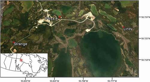
We captured frogs at three wetlands near the Churchill Northern Studies Centre: Lindy (58°43ʹ44ʹ’N, 93°46ʹ8’’W), Strange (58°43ʹ35ʹ’N, 93°50ʹ20ʹ’W), and Palsa 4 (58°44ʹ4’’N, 93°48ʹ35ʹ’W; Figure 1). These sites were chosen because wood frogs congregate at them to breed in the spring and because frogs tend to be present throughout the summer (Davenport, pers. obs.). Most importantly, however, we selected these wetlands because they represented a range of habitat characteristics, with each wetland varying in proportions of surrounding boreal forest and tundra habitats. For example, Lindy is an open tundra meadow site, with forest cover approximately 200 m from where frogs were captured. Palsa and Strange are areas with mixed tundra and forest, with patches of forest ≤50 m from where frogs were captured. Wood frogs were collected and tracked June–August of 2015 and 2016.

Figure 1. Location of three wetlands near Churchill, Manitoba, Canada, where we tracked the movements and habitat use of wood frogs

At all three wetland sites, adult wood frogs were collected opportunistically by hand or with unbaited minnow traps. Captured frogs were brought into a laboratory and fitted with a 0.4 g radio transmitter (Blackburn Transmitters, Nacogdoches, Texas, USA). We attached transmitters with a belt constructed from 0.7 mm stretch bead cord (Stretch Magic®, Pepperell Braiding Company, Pepperell, Massachusetts, USA) and used heat-shrink tubing to secure the knot (Groff et al. 2015). The belt and transmitter assembly represented between 3.2 and 6.5 percent (mean = 4.8%) of the mass of each individual (Appendix A). To ensure that the weight of the transmitter assembly was not a burden for the animals, we used animals that were larger than average for the region (see Davenport and Hossack 2016). Before release, the condition of all individuals was monitored overnight to assess belt fit.

We located radio-tagged frogs every other day using an R-1000 model receiver (Communications Specialists Inc., Orange, California, USA) and an RA-14 antenna (Telonics, Mesa, Arizona, USA). Frogs were tracked for an average of 16.8 d (range: 1–50 d). At least once per week, we checked frogs visually and removed the belt if abrasions developed. At the end of the tracking period, we removed the belt and transmitter from all frogs.

To estimate how frogs used terrestrial habitats, we recorded the position of each new relocation point (defined as a location where an animal stopped for a known duration) for frogs and determined the distance between successive locations (Groff, Calhoun, and Loftin 2017). This allowed us to measure total distance moved (sum of all movement paths) and net distance moved (straight-line distance from initial capture location) from the breeding wetland, and to estimate home-range size using the 100 percent minimum convex polygon (MCP) method (Miaud and Sanuy 2005; Mohr 1947) with the “minimum bounding geometry” tool in ArcGIS (ESRI v. 10.5, Redlands, California, USA). Also, we used mean daily temperatures and accumulated precipitation measured at the Churchill Airport (14.5 km from our study area) to determine if movement distances were related to weather conditions.

Each time a frog moved ≥3 m from the previous relocation point, we recorded microhabitat information on the ground cover of sedge, shrubs, trees, moss, lichen, standing water, and bare soil from a 1 m² plot surrounding the frog. To provide information on unused habitats, we also collected the same information from a randomly selected 1 m² plot paired with each relocation point. We determined the location of each random plot by using the same distance traveled from the previous relocation point but at a randomly assigned compass direction (Ryan and Calhoun 2014). For example, if a frog moved 10 m from its previous location, we selected a 1 m² plot that was 10 m from its new location and at a randomly chosen bearing between 1° and 360°.

Statistical analyses

To determine if there were differences in post-breeding movement distances between sexes and among populations (different wetlands), we used a generalized linear model with log-transformed response data fitted to the Gaussian distribution. We included the number of days each individual was tracked as a model covariate to account for the large range in these data (range: 4–50 d). For all analyses, individuals tracked ≤4 d were excluded from analyses. Total distance traveled, net distance traveled away from wetland, and home-range size were all strongly, positively correlated (Pearson’s r = 0.88–0.93), so we only compared total distance traveled. For these and subsequent models, we started with a model with the terms Wetland, Sex, and Days Tracked, and used backward selection to remove those parameters that did not differ from zero (P ≥ 0.05).

To determine the relationship between weather and movement distances, we tested the effect of accumulated precipitation (range: 0–79.8 mm) and mean temperature (range: 1.5–25.6°C) on distance moved (range: 0–185.3 m) between tracking locations with a generalized linear mixed model (R package lme4; Bates et al. 2015). We used a random intercept for each frog to account for repeated observations. Because these continuous data were dominated by zeros and were severely right-skewed, we added 0.01 to each value and fit the models to the Gamma distribution with a log link.

We used compositional analysis to determine if frogs spent a disproportionate amount of time in tundra or boreal forest habitats (R package adehabitat; Aebischer, Robertson, and Kenward 1993; Calenge 2006). Available habitat encompassed the amount of tundra and boreal forest habitat within a 400 m radius buffer around each wetland site where frogs were captured. We chose a radius of 400 m because 360 m (range: 8–360 m) was the longest net distance from a wetland that any frog moved. Notably, this frog was tracked for 15 d, less than the average of 16.8 d, and the greatest total distance moved by any frog was 808 m. We estimated habitat use by each frog by dividing the number of radio locations in each habitat by the total number of locations for that frog (Aebischer, Robertson, and Kenward 1993). If a frog did not use a particular habitat type, we replaced the proportion of use for that habitat type with 0.0001. All statistical analyses were performed in R 3.3.1 (R Development Core Team 2016).

Finally, we assessed the microhabitat use of frogs by comparing characteristics in 1 m² plots around relocation points (cases) for each frog to randomly selected 1 m² plots (controls). We assessed differences in percent cover by sedge, shrubs, moss, and standing water in used and random 1 m² plots with conditional logistic regression with a logic link (R package survival; Therneau 2015). Cover by lichens, trees, and bare soil was rare (<10%) and caused problems in model fitting, so these cover categories were excluded from analyses. None of the remaining microhabitat characteristics were strongly correlated (r = |0.13–0.47|). For this analysis, we stratified by pairs of case-control plots and by sex, and identified clusters based on unique frog identification to account for repeated observations of animals (Therneau and Grambsch 2013). We first fit an interactive model to determine if habitat use differed by sex and then eliminated nonsignificant terms to simplify the model.

Results

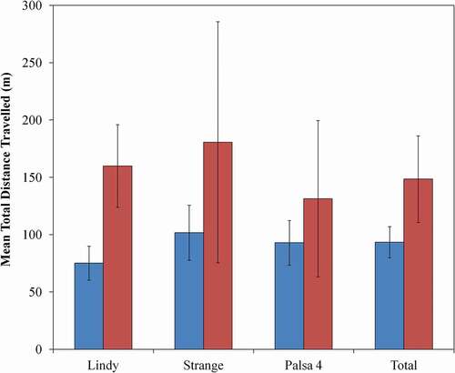
In 2015, we tracked sixteen frogs (eight males and eight females) at Lindy and twenty-one frogs (eighteen males and three females) at Strange. In 2016, we tracked twenty frogs (nine males and eleven females) at Palsa 4 (Table 1, Figure 2, Appendix A). The total distance traveled by individuals was strongly correlated only with the number of days that a frog was tracked (b_days = 0.033 [SE 0.009], F_1,54 = 12.16; P = 0.001). In general, females traveled farther than males (Figure 3), but the difference was not statistically significant (b_male = −0.273 [0.213], F_1,50 = 1.65, P = 0.205). Total distance traveled also did not vary among populations (F_2,53 = 1.76, P = 0.183). The distance moved between tracking locations ranged from 0 m to 185.3 m and, in relation to weather, distances increased with temperature (b_temp = 0.039 [0.018]; χ² = 4.67, df = 1, N = 494, P = 0.031) but were not associated with cumulative precipitation (b_precip = 0.013 [0.009]; χ² = 2.39, df = 1, N = 494, P = 0.122). Across all frogs, the size of the MCP home range averaged 1,326.19 m² (range: 5.0–19,256.5 m²); much of this variation was associated with the number of days a frog was tracked.

Table 1. Summary information for wood frogs tracked near Churchill, Manitoba, Canada, in 2015 and 2016

Wetland (Year)	Number of Each Sex Tracked (Females, Males)	Mean Number of Days Tracked (Range)	Mean Total Distance Traveled (m; Range)	Proportion of Habitat (Tundra, Forest) within 400 m of Wetland
Lindy (2015)	8, 9	18.0 (4–39)	117.5 (33.6–360.5)	0.96, 0.04
Strange (2015)	3, 18	11.7 (1–21)	112.9 (7.9–457.7)	0.76, 0.24
Palsa (2016)	11, 9	21.9 (2–50)	114.1 (29.2–807.9)	0.86, 0.14

Figure 2. Movement paths for wood frogs tracked near Churchill, Manitoba, Canada, in 2015 and 2016. We tracked sixteen frogs at Lindy (A), twenty-one frogs at Strange (B), and twenty frogs at Palsa 4 (C). For each wetland, an individual frog is represented by a unique combination of color and line style. Some individuals, such as those represented by the light-blue dotted line (B) and yellow dotted line (C), made movements away from and back to the wetland, and thus have a movement path that appears as a polygon

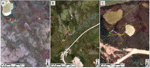
Figure 3. Mean total distance (m) traveled by radio-tracked male (blue bars; ± SE) and female (red bars; ± SE) wood frogs near three wetlands near Churchill, Manitoba, Canada. We tracked sixteen frogs (eight males and eight females) at Lindy, twenty-one frogs (eighteen males and three females) at Strange, and twenty frogs (nine males and eleven females) at Palsa 4

Based on available habitat within 400 m of each wetland, frogs used tundra habitats more than boreal forests (Wilk’s Λ = 0.067, P < 0.001). This strong difference occurred even though there was much more tundra than forest near wetlands. Only three frogs were ever relocated in the boreal forest. Two of these individuals were at Strange (2015), a female that was tracked for 9 d and moved 163 m total distance, and a male that was tracked for 18 d and moved 189 m total distance. At Palsa (2016), a male that was tracked for 44 d moved 127 m total distance and was found in boreal forest on three of the eight times it was located.

Across all individuals and sites, frogs used areas that had greater amounts of standing water and higher shrub and sedge cover more than expected, compared to paired random plots (Table 2). For every 1 percent increase in the cover of standing water, sedge, and shrubs, there was a 3.0, 3.7, and 4.6 percent increase in the odds of a frog using an area, respectively. Similar to distance traveled, we found weak evidence of differences in microhabitat use between sexes (χ² = 8.36, df = 5, P = 0.138).

Table 2. Odds ratios (robust 95% confidence intervals) and test statistics from the best-fit conditional logistic regression model of microhabitat selection (1 m² plots) by wood frogs near Churchill, Manitoba, Canada, in 2015 and 2016

Habitat Characteristic	Odds Ratio (95% CI)	χ^2 (df = 1)	Pr > χ^2
Standing water (%)	1.030 (1.013–1.047)	20.57	<0.001
Sedge (%)	1.037 (1.021–1.054)	33.11	<0.001
Shrubs (%)	1.046 (1.028–1.065)	39.92	<0.001

Discussion

Our results provide insight into important habitat features and post-breeding habitat use for wood frogs in a rapidly changing subarctic ecosystem. At the landscape scale, frogs spent a disproportionate amount of time in tundra over boreal forest. Even though the short tracking time of some frogs likely reduced their probability of reaching the forest because all wetlands were bordered by tundra, we also found little evidence for selection of trees at the microhabitat scale. The occurrence of trees in 1 m² plots where we located frogs (8.8%) was similar to that of randomly selected unused plots (6.1%). Furthermore, there were large patches of boreal forest within 50 m of both the Palsa and Strange wetlands, and based on tracking paths, frogs did not seem to actively seek those patches.

Unsurprisingly for a species with a huge geographical range, documented habitat associations have varied widely among studies. Across most of the species’ range in the contiguous United States, wood frogs are associated with dense stands of forest (Baldwin, Calhoun, and deMaynadier 2006; deMaynadier and Hunter 1998; Gibbs 1998). In Alaskan populations that bred in wetlands more than 1,000 m from boreal forest, wood frogs primarily used alder scrub tundra habitat after breeding (Hokit and Brown 2006). In a comparison of calling activity in different habitat types near Cape Churchill, Manitoba, wood frogs seemed equally abundant in sedge meadows and the boreal forest–tundra transition zone (Reiter, Boal, and Andersen 2008). Although the distribution of wood frogs at northern latitudes largely tracks the treeline (Dodd 2013), our results and those of Reiter, Boal, and Andersen (2008) suggest that the frogs may not be dependent on or even select boreal forest habitats, at least during the summer.

Movement patterns of frogs in our study were influenced by temperature but not by precipitation. Amphibians often make longer distance movements during favorable weather conditions, such as warm rainfall events, especially where water is a limited resource (Bartelt, Peterson, and Klaver 2004; Rittenhouse, Semlitsch, and Thompson 2009; Ryan and Calhoun 2014). However, our study area is distinct from many other sites because pooled water is abundant throughout the summer. Many wetlands in our area are also interconnected, which likely further facilitates movement across the landscape. Melting permafrost in the region is a long-term threat to tundra ecosystems and water budgets (Riordan, Verbyla, and McGuire 2006; Wolfe et al. 2011; Yoshikawa and Hinzman 2003), but in the near term we suspect that melting permafrost might aid the movement of semiaquatic organisms such as frogs. For example, of the twelve documented movements that were more than 100 m, eleven occurred after July 15, during the peak of summer heat and drought. In general, we suspect that wood frog populations in the Subarctic are less limited by desiccation risk than southern, temperate populations.

Despite the short time period during which we tracked many frogs, the distances moved and home range sizes we documented are as large as many of those reported for southern wood frog populations. The previous maximum distances traveled by wood frogs ranged from 340 m to 569 m (Baldwin, Calhoun, and deMaynadier 2006; Groff, Calhoun, and Loftin 2017; Rittenhouse and Semlitsch 2009). In our study, we had a female from Palsa move 808 m during the 50 d she was tracked. In many telemetry studies of frogs and toads, distance traveled or habitat use differs between sexes (e.g., Bartelt, Peterson, and Klaver 2004; Regosin, Windmiller, and Reed 2003; Rittenhouse and Semlitsch 2007). Although females moved farther than males on average at all wetlands in our study, there was extensive variation among individuals, and the differences attributable to sex did not differ from zero.

The short active periods for many species that inhabit areas with cold climates imposes severe energy constraints that might affect movement and home-range sizes (Carfagno and Weatherhead 2008; McNab 1963). For example, wood frogs in interior Alaska and the montane landscapes of Maine may be active for less than 150 d per year (Groff, Calhoun, and Loftin 2016; Larson et al. 2014); we suspect that the active season in our study area, which has a shorter growing season, is similar if not shorter than for these previous two studies (Davenport and Hossack 2016). Resource needs likely affect seasonal movements even within years. In a Maine population of wood frogs, home-range sizes were larger in the autumn than in the spring, possibly related to the need to acquire energetic resources before overwintering (Blomquist and Hunter 2010). In our study area, it is possible that the demand to acquire enough energy resources to sustain the long hibernation period contributed to the comparatively large travel distances that we documented. Further research is needed to quantify movement behavior and the energy acquisition and expenditure of wood frogs during the growing seasons across their large geographic range.

Climate change has the potential to have both negative and positive effects on northern populations of wood frogs and other vertebrates. For example, the selection for shrubs in our study area may be advantageous for adult wood frogs as temperatures continue to rise and aid the growth and northward expansion of shrubs (Danby and Hik 2007; Myers-Smith et al. 2011). There are trade-offs with these potentially beneficial changes, however. Increases in shrub communities will likely be accompanied by the accelerated drying of wetlands (Macrae et al. 2014; Riordan, Verbyla, and McGuire 2006; Wolfe et al. 2011), which could limit the time wood frogs and other species with complex life histories have to metamorphose. Evidence suggests that local wood frogs have limited, but incomplete, capacity to adapt to reduced hydroperiods by decreasing their time to metamorphosis, with minimal reductions in size at metamorphosis (Davenport, Hossack, and Fishback 2017). But there will be a limit to this adaptability, and the effects of these changes on terrestrial life stages are still unknown (Benard 2015). With the dynamic nature of climate change and potentially opposing effects on different life stages, detailed, long-term data across life stages will be required to measure the local and regional changes to populations.

Acknowledgments

We thank A. Feltmann, A. King, K. Thomson, K. Mills, and Earthwatch Institute participants from the summers of 2015 and 2016 for their assistance in the field. We also thank L. Groff for sharing information on field techniques and for providing comments on the manuscript, as well as T. Hastings for helping to tie up loose ends.

Disclosure statement

No potential conflict of interest was reported by the authors.

Additional information

Funding

The Churchill Northern Studies Centre provided funding under the Northern Research Fund and logistical support. Additional funding was provided by Earthwatch Institute, Theodore Roosevelt Memorial Fund of the American Museum of Natural History, the Explorers Club Exploration Fund-Mamont Scholars Program, and (to B. Hossack) the U.S. Geological Survey Amphibian Research and Monitoring Initiative (ARMI). This manuscript is ARMI contribution no. 621. Any use of trade, product, or firm names is for descriptive purposes only and does not imply endorsement by the U.S. Government. Frogs were tracked and handled in accordance with the Manitoba Conservation and Water Stewardship permit WB17529 to J.M.D.

Appendix A

Summary of radiotracking data and individual metrics for fifty-seven wood frogs tracked June–August 2015 and 2016

Frog ID	Sex	Mass (g)	SVL (mm)	Site	Dates Tracked	Number of Locations	Total Days Tracked	Longest Net Distance (m)	Total Distance Moved (m)	Home-range Size (m^2)
1	F	12.01	57	Lindy 5	6/3/15–6/7/15	3	4	43.48	84.80	763.50
2	F	9.21	51	Lindy 5	6/7/15–7/16/15	10	39	48.35	149.65	855.50
3	F	9.20	56	Lindy 5	6/7/15–7/16/15	9	39	233.45	257.17	4,436.00
4	F	9.00	55	Lindy 5	7/3/15–7/19/15	4	16	60.03	136.21	237.00
5	F	12.50	55	Lindy 5	7/3/15–7/16/15	3	13	131.59	154.50	1,970.00
6	F	12.45	54	Lindy 5	7/14/15–7/29/15	3	15	56.11	64.38	203.50
7	F	11.34	54	Lindy 5	7/14/15–7/29/15	7	15	32.46	72.13	474.50
8	F	9.79	50	Lindy 5	7/18/15–7/29/15	3	11	338.02	360.52	8,258.50
9	F	7.64	47	Strange	7/22/15–8/6/15	5	15	360.13	370.99	4,357.50
10	F	10.28	52	Strange	8/8/15–8/17/15	5	9	149.09	162.71	1,425.00
11	F	12.01	44	Strange	8/12/15–8/17/15	2	5	7.81	7.85	5.00
12	M	9.19	48	Lindy 5	6/3/15–6/23/15	5	20	23.10	47.82	65.00
13	M	8.24	47	Lindy 5	6/4/15–6/25/15	7	21	117.13	150.40	1,079.50
14	M	7.37	45	Lindy 5	6/5/15–6/25/15	5	20	22.03	65.87	83.00
15	M	7.06	44	Lindy 5	6/6/15–6/29/15	5	23	35.00	72.30	150.00
16	M	7.77	42	Lindy 5	6/17/15–7/3/15	4	16	36.69	42.70	49.50
17	M	7.83	46	Lindy 5	6/23/15–7/3/15	2	10	27.18	33.60	64.50
18	M	7.87	48	Lindy 5	7/7/15–7/21/15	5	14	35.17	59.90	163.50
19	M	9.07	50	Lindy 5	7/7/15–7/19/15	4	12	117.76	128.28	1,244.50
20	M	6.13	44	Strange	6/26/15–7/2/15	1	6	56.04	56.04	112.10
21	M	7.63	46	Strange	6/26/15–7/13/15	7	17	100.13	141.99	1,492.50
22	M	7.18	47	Strange	6/27/15–7/11/15	5	14	39.61	58.12	98.00
23	M	6.68	46	Strange	7/2/15–7/15/15	4	13	29.44	43.62	123.50
24	M	9.78	53	Strange	7/11/15–7/20/15	3	9	56.63	105.73	1,290.50
25	M	9.55	50	Strange	7/13/15–7/26/15	6	13	36.09	65.07	400.00
26	M	7.50	48	Strange	7/17/15–8/4/15	5	18	29.44	84.59	108.00
27	M	8.10	48	Strange	7/22/15–8/6/15	1	15	43.42	43.42	86.80
28	M	9.33	49	Strange	7/22/15–8/4/15	5	13	260.51	457.68	19,256.50
29	M	9.50	50	Strange	7/22/15–7/31/15	3	9	21.41	23.64	48.50
30	M	8.60	47	Strange	7/22/15–8/12/15	8	21	54.84	144.83	496.50
31	M	7.33	46	Strange	7/22/15–8/9/15	6	18	92.88	189.17	1,260.50
32	M	6.92	45	Strange	7/24/15–8/6/15	4	13	29.44	41.90	126.00
33	M	6.97	46	Strange	7/24/15–8/9/15	6	16	88.67	154.14	819.00
34	M	7.75	47	Strange	8/6/15–8/17/15	2	11	32.03	42.62	136.00
35	M	7.74	44	Strange	8/12/15–8/17/15	2	5	68.29	112.36	879.00
36	M	7.06	47	Strange	8/12/15–8/13/15	1	1	24.02	24.02	48.00
37	M	7.21	46	Strange	8/12/15–8/17/15	3	5	35.24	41.01	146.00
38	F	7.77	49	Palsa 4	6/15/16–6/17/16	1	2	33.24	33.24	66.48
39	F	8.04	55	Palsa 4	6/15/16–8/4/16	19	50	163.28	807.87	11,432.50
40	M	6.96	47	Palsa 4	6/15/16–7/4/16	7	19	36.37	85.25	510.50
41	F	7.39	46	Palsa 4	6/16/16–7/17/16	5	31	36.91	51.25	174.50
42	M	8.05	48	Palsa 4	6/16/16–7/28/16	8	44	47.87	127.04	657.00
43	F	9.54	54	Palsa 4	6/17/16–7/15/16	3	28	106.44	113.61	916.50
44	M	8.11	49	Palsa 4	6/16/16–7/8/16	9	22	144.01	213.61	2,543.00
45	M	8.23	46	Palsa 4	6/21/16–7/10/16	7	19	30.88	46.84	249.00
46	M	7.67	46	Palsa 4	6/22/16–8/1/16	11	40	43.34	80.69	335.00
47	F	8.29	48	Palsa 4	6/22/16–7/15/16	5	23	38.29	55.73	140.50
48	F	10.41	54	Palsa 4	6/23/16–7/8/16	2	15	26.26	29.25	10.00
49	M	8.10	48	Palsa 4	6/25/16–8/1/16	12	37	40.33	142.69	447.50
50	F	9.22	50	Palsa 4	6/26/16–7/17/16	6	21	35.00	43.57	85.00
51	F	10.34	49	Palsa 4	7/9/16–7/19/16	4	10	30.90	52.44	244.50
52	F	7.45	46	Palsa 4	7/9/16–7/30/16	8	21	36.69	97.81	850.50
53	F	10.38	48	Palsa 4	7/9/16–7/24/16	4	15	29.44	59.09	458.00
54	M	8.62	49	Palsa 4	7/16/16–7/28/16	4	12	33.13	62.60	273.00
55	M	7.66	46	Palsa 4	7/22/16–8/4/16	3	13	34.90	40.63	125.50
56	M	9.02	49	Palsa 4	7/22/16–7/28/16	2	6	33.55	36.89	120.00
57	F	11.71	52	Palsa 4	7/25/16–8/4/16	4	10	60.90	101.45	603.00

References

- Aebischer, N. J., P. A. Robertson, and R. E. Kenward. 1993. Compositional analysis of habitat use from animal radio-tracking data. Ecology 74:1–9.
- Anthelme, F., L. A. Cavieres, and O. Dangles. 2014. Facilitation among plants in alpine environments in the face of climate change. Frontiers in Plant Science 5:387.
- Baldwin, R. F., A. J. K. Calhoun, and P. G. deMaynadier. 2006. Conservation planning for amphibian species with complex habitat requirements: A case study using movements and habitat selection of the wood frog Rana sylvatica. Journal of Herpetology 40:442–53.
- Bartelt, P. E., C. R. Peterson, and R. W. Klaver. 2004. Sexual differences in the post-breeding movements and habitats selected by western toads (Bufo boreas) in southeastern Idaho. Herpetologica 60:455–67.
- Bates, D., M. Mächler, B. M. Bolker, and S. C. Walker. 2015. Fitting linear mixed-effects models using lme4. Journal of Statistical Software 67:1–48.
- Benard, M. 2015. Warmer winters reduce frog fecundity and shift breeding phenology, which consequently alters larval development and metamorphic timing. Global Change Biology 21:1058–65.
- Blomquist, S. M., and M. L. Hunter. 2010. A multi-scale assessment of amphibian habitat selection: Wood frog response to timber harvesting. Ecoscience 17:251–64.
- Both, C., S. Bouwhuis, C. M. Lessells, and M. E. Visser. 2006. Climate change and population declines in a long-distance migratory bird. Nature 441:81–83.
- Brandson, L. 2011. Churchill Hudson Bay: A guide to natural and cultural heritage. Churchill: The Churchill Eskimo Museum. 384.
- Calenge, C. 2006. The package ‘adehabitat’ for the R software: A tool for the analysis of space and habitat use by animals. Ecological Modelling 197:516–19.
- Carfagno, G. L. F., and P. J. Weatherhead. 2008. Energetics and space use: Intraspecific and interspecific comparisons of movements and home ranges of two Colubrid snakes. Journal of Animal Ecology 77:416–24. doi:https://doi.org/10.1111/j.1365-2656.2008.01342.x.
- Chen, I.-C., J. K. Hill, R. Ohlemüller, D. B. Roy, and C. D. Thomas. 2011. Rapid range shifts of species associated with high levels of climate warming. Science 333:1024–26.
- Cohen, J., J. A. Screen, J. C. Furtado, M. Barlow, D. Whittleston, D. Coumou, J. Francis, K. Dethloff, D. Entekhabi, J. Overland, et al. 2014. Recent Arctic amplification and extreme mid-latitude weather. Nature Geoscience 7:627–37.
- Danby, R. K., and D. S. Hik. 2007. Variability, contingency and rapid change in recent subarctic alpine tree line dynamics. Journal of Ecology 95:352–63.
- Davenport, J. M., and B. R. Hossack. 2016. Reevaluating geographic variation in life-history traits of a widespread Nearctic amphibian. Journal of Zoology 299:304–10.
- Davenport, J. M., B. R. Hossack, and L. Fishback. 2017. Additive impacts of experimental climate change increase risk to an ectotherm at the Arctic’s edge. Global Change Biology 23:2262–71.
- deMaynadier, P. G., and M. L. Hunter. 1998. Effects of silvicultural edges on the distribution and abundance of amphibians in Maine. Conservation Biology 12:340–52.
- Dodd, C. K. 2013. Frogs of the United States and Canada. Baltimore: The Johns Hopkins University Press. 982.
- Dulvy, N. K., S. I. Rogers, S. Jennings, V. Stelzenmüller, S. R. Dye, and H. R. Skjoldal. 2008. Climate change and deepening of the North Sea fish assemblage: A biotic indicator of warming seas. Journal of Applied Ecology 45:1029–39. doi:https://doi.org/10.1111/j.1365-2664.2008.01488.x.
- Fraser, L. H., and P. A. Keddy. 2005. The World’s largest Wetlands: Ecology and conservation. Cambridge: Cambridge University Press, 488 pp.
- Gibbs, J. P. 1998. Distribution of woodland amphibians along a forest fragmentation gradient. Landscape Ecology 13:263–68.
- Groff, L. A., A. J. K. Calhoun, and C. S. Loftin. 2016. Hibernal habitat selection by wood frogs (Lithobates sylvaticus) in a northern New England montane landscape. Journal of Herpetology 50:559–69. doi:https://doi.org/10.1670/15-131R1.
- Groff, L. A., A. J. K. Calhoun, and C. S. Loftin. 2017. Amphibian terrestrial habitat selection and movement patterns vary with annual life-history period. Canadian Journal of Zoology 95:433–42. doi:https://doi.org/10.1139/cjz-2016-0148.
- Groff, L. A., A. L. Pitt, R. F. Baldwin, A. J. K. Calhoun, and C. S. Loftin. 2015. Evaluation of a waistband for attaching external radio transmitters to anurans. Wildlife Society Bulletin 39:610–15. doi:https://doi.org/10.1002/wsb.554.
- Harsch, M., P. Hulme, M. McGlone, and R. Duncan. 2009. Are treelines advancing? A global meta-analysis of treeline response to climate warming. Ecology Letters 12:1040–49.
- Hersteinsson, P., and D. W. MacDonald. 1992. Interspecific competition and the geographical distribution of red and arctic foxes Vulpes vulpes and Alopex lagopus. Oikos 64:505–15.
- Hokit, D. G., and A. Brown. 2006. Distribution patterns of wood frogs (Rana sylvatica) in Denali National Park. Northwestern Naturalist 87:128–37.
- IPCC. 2014: Climate Change 2014: Synthesis Report. Contribution of Working Groups I, II and III to the Fifth Assessment Report of the Intergovernmental Panel on Climate Change (eds. Core Writing Team, Pachauri, R.K., Meyer, L.A.). Geneva: IPCC, 151 pp.
- Lantz, T. C., P. Marsh, and S. V. Kokelj. 2013. Recent shrub proliferation in the Mackenzie Delta Uplands and microclimatic implications. Ecosystems 16:47–59.
- Larson, D. J., L. Middle, H. Vu, W. Zhang, A. S. Serianni, J. Duman, and B. M. Barnes. 2014. Wood frog adaptations to overwintering in Alaska: New limits to freezing tolerance. The Journal of Experimental Biology 217:2193–200.
- MacDonald, L. A., N. Farquharson, G. Merritt, S. Fooks, A. S. Medeiros, R. I. Hall, B. B. Wolfe, M. L. Macrae, and J. N. Sweetman. 2015. Limnological regime shifts caused by climate warming and lesser snow goose population expansion in the western Hudson Bay Lowlands (Manitoba, Canada). Ecology and Evolution 5:921–39.
- Macrae, M. L., L. C. Brown, C. R. Duguay, J. A. Parrott, and R. M. Petrone. 2014. Observed and projected climate change in the Churchill region of the Hudson Bay Lowlands and implications for pond sustainability. Arctic, Antarctic, and Alpine Research 46:272–85.
- McNab, B. K. 1963. Bioenergetics and the determination of home range size. The American Naturalist 97:133–40.
- Miaud, C., and D. Sanuy. 2005. Terrestrial habitat preferences of the natterjack toad during and after the breeding season in a landscape of intensive agricultural activity. Amphibia-Reptilia 26:359–66.
- Mohr, C. O. 1947. Table of equivalent populations of North American small mammals. The American Midland Naturalist 37:223–49.
- Myers-Smith, I. H., B. C. Forbes, M. Wilmking, M. Hallinger, T. Lantz, D. Blok, K. D. Tape, M. Macias-Fauria, U. Sass-Klassen, E. Lévesque, et al. 2011. Shrub expansion in tundra ecosystems: Dynamics, impacts and research priorities. Environmental Research Letters 6:045509.
- Post, E., M. C. Forchhammer, M. S. Bret-Harte, T. V. Callaghan, T. R. Christensen, B. Elberling, A. D. Fox, G. Olivier, D. S. Hik, T. T. Høye, et al. 2009. Ecological dynamics across the Arctic associated with recent climate change. Science 325:1355–58. doi:https://doi.org/10.1126/science.1173113.
- Quinton, W. L., M. Hayashi, and L. E. Chasmer. 2011. Permafrost-thaw-induced land-cover change in the Canadian subarctic: Implications for water resources. Hydrological Processes 25:152–58.
- R Development Core Team. 2016. R: A language and environment for statistical computing. Version 3.3.1 [computer program]. Vienna, Austria: R Foundation for Statistical Computing.
- Regosin, J. V., B. S. Windmiller, and J. M. Reed. 2003. Terrestrial habitat use and winter densities of the wood frog (Rana sylvatica). Journal of Herpetology 37:390–94.
- Reiter, M. E., C. W. Boal, and D. E. Andersen. 2008. Anurans in a Subarctic tundra landscape near Cape Churchill, Manitoba. Canadian Field-Naturalist 122:129–37.
- Riordan, B., D. Verbyla, and A. D. McGuire. 2006. Shrinking ponds in subarctic Alaska based on 1950-2002 remotely sensed images. Journal of Geophysical Research: Biogeosciences 111:G04002.
- Rittenhouse, T. A. G., and R. D. Semlitsch. 2007. Distribution of amphibians in terrestrial habitat surrounding wetlands. Wetlands 27:153–61.
- Rittenhouse, T. A. G., and R. D. Semlitsch. 2009. Behavioral response of migrating wood frogs to experimental timber harvest surrounding wetlands. Canadian Journal of Zoology 87:618–25.
- Rittenhouse, T. A. G., R. D. Semlitsch, and F. R. Thompson III. 2009. Survival costs associated with wood frog breeding migrations: Effects of timber harvest and drought. Ecology 90:1620–30.
- Ross, M. V., R. T. Alisauskas, D. C. Douglas, and D. K. Kellett. 2017. Decadal declines in avian herbivore reproduction: Density-dependent nutrition and phenological mismatch in the Arctic. Ecology 98:1869–83.
- Rouse, W. R., M. S. V. Douglas, R. E. Hecky, A. E. Hershey, G. W. Kling, L. Lesack, P. Marsh, M. McDonald, B. J. Nicholson, N. T. Roulet, et al. 1997. Effects of climate change on the freshwaters of Arctic and Subarctic North America. Hydrological Processes 11:873–902.
- Ryan, K. J., and A. J. K. Calhoun. 2014. Postbreeding habitat use of the rare, pure-diploid blue-spotted salamander (Ambystoma laterale). Journal of Herpetology 48:556–66. doi:https://doi.org/10.1670/13-204.
- Saino, N., R. Ambrosini, D. Rubolini, J. Von Hardenberg, A. Provenzale, K. Hüppop, O. Hüppop, A. Lehikoinen, E. Lehikoinen, K. Rainio, et al. 2011. Climate warming, ecological mismatch at arrival and population decline in migratory birds. Proceedings of the Royal Society B: Biological Sciences 278:835–42. doi:https://doi.org/10.1098/rspb.2010.1778.
- Schriever, T. A., and D. D. Williams. 2013. Ontogenetic and individual diet variation in amphibian larvae across an environmental gradient. Freshwater Biology 58:223–36.
- Scott, G. A. J. 1995. Canada’s vegetation: A world perspective. Montreal: McGill-Queen’s Press, 404
- Serreze, M. C., and J. A. Francis. 2006. The Arctic amplification debate. Climatic Change 76:241–64.
- Smol, J. P., and M. S. V. Douglas. 2007. Crossing the final ecological threshold in high Arctic ponds. Proceedings of the National Academy of Sciences of the United States of America 104:12395–97.
- Stickney, A. A., T. Obritschkewitsch, and R. M. Burgess. 2014. Shifts in fox den occupancy in the greater Prudhoe Bay area, Alaska. Arctic 67:196–202.
- Stuart, S. N., J. S. Chanson, N. A. Cox, B. E. Young, A. S. L. Rodrigues, D. L. Fischman, and R. W. Waller. 2004. Status and trends of amphibian declines and extinctions worldwide. Science 306:1783–86. doi:https://doi.org/10.1126/science.1103538.
- Therneau, T. M. 2015: A package for survival analysis in S. version 2.38. Accessed September 13, 2017. https://cran.r-project.org/web/packages/survival/citation.html.
- Therneau, T. M., and P. M. Grambsch. 2013. Modeling Survival Data: Extending the Cox Model. New York: Springer. 350.
- Wolfe, B. B., E. M. Light, M. L. MacRae, R. I. Hall, K. Eichel, S. Jasechko, J. White, L. Fishback, and T. W. D. Edwards. 2011. Divergent hydrological responses to 20th century climate change in shallow tundra ponds, western Hudson Bay Lowlands. Geophysical Research Letters 38: L23402. 1-L23402.6. doi:https://doi.org/10.1029/2011GL049766.
- Yoshikawa, K., and L. D. Hinzman. 2003. Shrinking thermokarst ponds and groundwater dynamics in discontinuous permafrost near Council, Alaska. Permafrost and Periglacial Processes 14:151–60.