Elevation changes of the Holm Land Ice Cap, northeast Greenland, from 1978 to 2012–2015, derived from high-resolution digital elevation models

ABSTRACT

Greenland’s peripheral glaciers and ice caps are key indicators of climate change in the Arctic, but quantitative observational data of their recent evolution are sparse. Three recently released high-resolution digital elevation models (DEMs)—AeroDEM (based on images from 1978 to 1987), ArcticDEM (2012–2015), and TanDEM-X (2010–2014)—provide the possibility to calculate elevation changes spanning almost four decades along the margins of the Greenland Ice Sheet. This study explores the potential of these DEMs by calculating elevation changes for the Holm Land Ice Cap (865 km²), northeast Greenland. Co-registration indicated no significant shifts between the DEMs but we encountered localized vertical offsets in AeroDEM. The data quality of ArcticDEM and TanDEM-X is high, but AeroDEM suffers from 19 percent low-quality data, which were treated as data voids. Applying two approaches to fill the data voids in the difference grid between ArcticDEM and AeroDEM, mean surface-elevation change over the Holm Land Ice Cap and a period of approximately 35 y is in the range of −8.30 ±0.30 m. Comparing ArcticDEM and TanDEM-X reveals a glacier elevation difference of 2.54 m, which may be partly related to the different retrieval techniques (optical and SAR). Overall, the DEMs have good potential for large-scale and long-term assessment of geodetic glacier mass balance.

KEYWORDS:

• glacier elevation change
• digital elevation models
• ArcticDEM
• TanDEM-X
• northeast Greenland

Introduction

Greenland peripheral glaciers and ice caps cover only about 5 percent of the glacierized area of Greenland but they are responsible for a substantial fraction (14–20%) of the total ice loss from Greenland between October 2003 and March 2008 (Bolch et al. 2013). These glaciers respond faster to climate change than the ice sheet and are key indicators of the climate in the Arctic. Additionally, their potential contribution to sea-level rise makes detailed studies of their spatial and temporal evolution essential (Machguth et al. 2013; Noël et al. 2017). Mass-balance studies of individual glaciers indicate substantial variability across Greenland, ranging from pronounced mass loss (e.g., Mittivakkat Glacier, Mernild et al. 2011) to near-equilibrium (Flade Isblink Ice Cap, Rinne et al. 2011). These contrasting results call for a large-scale assessment of the current state of Greenland’s periphery (Bjørk et al. 2018).

In situ mass-balance measurements on Greenland’s peripheral glaciers are essential for model calibration and validation (e.g., Noël et al. 2017) but they are sparse and often limited to short-lived measuring programs (Machguth et al. 2016). Therefore, it is also worthwhile to assess mass-balance changes of Greenland’s peripheral glaciers with the geodetic method.

Geodetic surveys of glacier thickness change are based on subtracting two digital elevation models (DEMs) from two different dates. The method has the advantage of being applicable to extended areas. Also, it can be applied retrospectively, provided historical DEMs exist or become available. To present, Greenland’s peripheral glaciers have seen the application of the geodetic approach either on small individual glaciers (Marcer et al. 2017; Yde et al. 2014) or over relatively short time periods (e.g., 2002–2009; Rinne et al. 2011). Bolch et al. (2013) used satellite altimetry from ICESat to assess ice-thickness change for all peripheral glaciers of Greenland but the survey period is short (2003–2008). Furthermore, the scanning characteristics of the ICESat laser altimeter with large horizontal gaps between the scanning tracks are not optimal to measure changes on smaller glaciers, requiring a substantial amount of interpolation and introducing potentially large uncertainties. A study by Bjørk et al. (2018) provides valuable long-term observations, covering a time period from 1890 to today, but focuses on glacier length fluctuations in east (70.5–75.0 °N) and west (71.0–72.5 °N) Greenland.

Recently, three new DEMs became available, opening up the possibility to geodetically measure the volume changes of Greenland’s peripheral glaciers during the past approximately forty years. The AeroDEM model (Korsgaard et al. 2016) dates to the time period 1978–1987 and covers all of Greenland’s periphery. The ArcticDEM model (Polar Geospatial Center, Morin et al. 2016) comprises the time period 2012–2015 and covers most of the Arctic. The TanDEM-X DEM (hereafter TanDEM-X, German Aerospace Center) is available globally and dates from 2010 to 2014. In contrast to other DEMs that cover northern Greenland (e.g., GIMP DEM, Aster GDEM v2), AeroDEM, ArcticDEM, and TanDEM-X offer higher spatial resolution and their time stamps are better constrained.

Here, we make use of the newly available data to calculate glacier elevation changes over the Holm Land Ice Cap, northeast Greenland, and evaluate the potential and limitations of the newly available DEMs. We aim at creating knowledge on long-term ice-volume changes in a part of Greenland that lacks such studies.

Data and study site

Digital elevation models

We used three different DEMs covering the peninsula of Holm Land. (1) The AeroDEM represents surface elevations over Holm Land in 1978 at 25 m spatial resolution and is based on aerial photographs. AeroDEM heights are given relative to the WGS 84 ellipsoid and are externally validated using ICESat altimetry from the GLA12 Release 31. Co-registration to the ICESat data revealed an accuracy of 10 m horizontally and 6 m vertically (Korsgaard et al. 2016). (2) The ArcticDEM (Polar Geospatial Center, Morin et al. 2016) has a spatial resolution of 5 m and has been compiled from approximately 0.5 m resolution WorldView optical satellite images. The strips of the ArcticDEM used are based on satellite images taken on August 23, 2013, and on June 17, 2012 (Table 1). Data voids in these two base files were filled during the DEM creation with information from images taken between 2012 and 2015. Because those former voids are not indicated to the user, they prevent a more exact dating of the ArcticDEM than 2013 ±2 y. Height is stated relative to the WGS 84 ellipsoid. Internal (pixel to pixel) accuracy is high (0.2 m, Noh and Howat 2015), and absolute accuracy is better than 4 m in the presence of ground control. The files used for this study were co-registered using ground-control points from ICESat altimetry from the GLA12 Release 34. (3) The TanDEM-X represents surface elevation at 12 m resolution and is derived from SAR-processed X-band satellite imagery that was taken between 2010 and 2014. Heights represent weighted height averages of all data contributing to a scene, weighted inversely to their respective error (Gruber et al. 2016). We therefore date the TanDEM-X to 2012 ±2 y. The heights are stated relative to the WGS 84 ellipsoid. The TanDEM-X was validated using tie points (overlapping areas of neighboring scenes). A correction based on ICESat was not applied on ice caps in Greenland to avoid an uplift resulting from the different scattering planes. The absolute horizontal and vertical resolution of the TanDEM-X is specified as less than 10 m (Wessel 2016). The data used in this study are summarized in Table 1.

Table 1. Overview of DEMs used in this study. Base file refers to the main satellite scenes that were used to establish the strips of the ArcticDEM used in this study

DEM Name	Reference Date	Grid Size (m)	File Names of Strips Used	Accuracy (m) Horizontal/Vertical	Validation
AeroDEM	1978	25	aerodem_1978_utm27N	10/6	ICESat
ArcticDEM	2012–2015	5		< 4/4	ICESat
Base file	08/23/2013		31_45_2_1, 31_45_2_2
Base file	06/17/2012		31_46_1_1, 31_46_1_2
TanDEM-X	2010–2014	12	04_N80W020_DEM	< 10/10	Tie points

Holm Land, northeast Greenland

The choice of our study site is based on identifying regions of Greenland’s periphery with high-quality data. Depending on the retrieval technique, the quality of DEMs suffers from low contrast (snow cover), atmospheric obstructions such as clouds, and geometrical effects of the viewing geometry such as shadows (Korsgaard et al. 2016). TanDEM-X and ArcticDEM are built of data from multiple overflights, increasing the chance of a successful retrieval and resulting in almost complete data sets. Therefore, limitations in the sense of limited data quality were mainly given by the AeroDEM. Looking at the entire periphery of Greenland, 50 percent of the surface could not be successfully resolved in the AeroDEM (Korsgaard et al. 2016). One of the exceptions is Holm Land, a peninsula of approximately 1,300 km² located in northeast Greenland (80 °N, 18 °W, Figure 1) that is named after Danish naval officer and Arctic explorer Gustav Frederik Holm. The AeroDEM over the study area has relatively few low-quality values (19 percent of the glacier surface). Its proximity to the ice cap of Flade Isblink, for which mass-balance estimates have been established recently, enables meaningful comparisons (Rinne et al. 2011).

Figure 1. The Holm Land Ice Cap as seen from Sentinel-2 (ESA) on August 26, 2016. The approximate outlines of the peninsula are overlain with glacier outlines modified from the Greenland glacier inventory by Rastner et al. (2012). The largest glaciers are numbered according to their identification in the Randolph Glacier Inventory (RGI Consortium 2017)

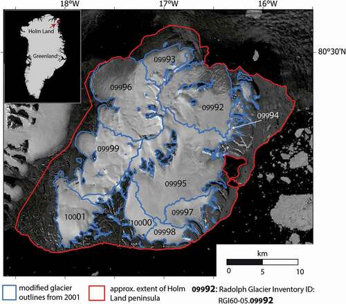
Two-thirds of the peninsula is covered by the Holm Land Ice Cap, which has an area of 865 km² (Rastner et al. 2012). The Greenland glacier inventory by Rastner et al. (2012) lists twenty-five glaciers and glacierets on Holm Land that extend from sea level to 1,100 m a.s.l., with a median elevation of 465 m. The Greenland glacier inventory divides the main ice cap into ten larger glaciers.

Here we use modified glacier outlines from the Greenland glacier inventory by Rastner et al. (2012) as available through GLIMS and the Randolph Glacier Inventory (RGI) as glacier mask. We compared original outlines (based on glacier extent in 2001) from Rastner et al. (2012) to a Sentinel-2 image from August 26, 2016 (Figure 1), and noticed an offset of approximately 70 m between the shapefiles and the actual glacier extent according to the Sentinel-2 image. The reasons for this shift (also found when comparing to the original Landsat imagery) are unknown. Therefore, for this study we manually shifted the outlines from Rastner et al. (2012) to the glacier extent as visible on the Sentinel-2 image.

We manually mapped glacier extent as seen in the Sentinel-2 image from 2016 and in the orthorectified photos from 1978 and compared it to the total area as indicated by the glacier mask (in 2001). Area changes were less than 2 percent (2001–2016) and 0.6 percent (1978–2001) of the total glaciarized area. No large elevation changes are observed outside of the glacier outlines of 2001, indicating that they are a valid mask to assess glacier volume changes over the full time period. For distinction the glaciers were given numbers according to their RGI identification number (RGI Consortium 2017).

Methods

Preprocessing

All three DEMs (AeroDEM, ArcticDEM, TanDEM-X) were re-projected to WGS 1984 UTM zone 27N. Subsequently, the DEMs were re-sampled to a common resolution; that is, 25 m for the comparison of AeroDEM and ArcticDEM and 12 m for ArcticDEM and TanDEM-X, respectively. As the interpolation method, bi-linear interpolation was used following Nuth and Kääb (2011).

Although the quality of AeroDEM over Holm Land (19 percent low-quality data) is better than for other parts of Greenland, the DEM suffers from frequent low-quality values mainly in the accumulation area of the glaciers (Korsgaard et al. 2016). To assess the quality of the data points, a reliability mask (RM) is available that contains the Figure of Merit (FOM) value that differentiates between measured and interpolated pixels. As recommended for elevation changes, all interpolated pixels were masked out and assigned a “no data” value (Korsgaard et al. 2016).

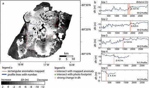
An initial examination of DEM quality was done using hillshade DEMs, visual inspection along transects, shifts in contour lines, and analysis of Δh grids. Figure 2a shows artifacts in the AeroDEM on the example of a Δh grid. We observed sudden changes in surface elevation ranging from 5 m to 9 m (Figure 2b). These artifacts appear to coincide with the extent of some of the aerial photographs used to calculate the AeroDEM. We assume that small errors in the image alignment in the automated photogrammetric workflow have caused the artifacts.

Figure 2. Analysis of artifacts in the AeroDEM. (a) Elevation-change grid (Δh, ArcticDEM minus AeroDEM) with step-wise changes in Δh highlighted in red and numbered transects. (b) Transects of the Δh grid with values indicated at the sudden Δh changes

Co-registration

Co-registration is essential before assessing differences between DEMs (e.g., Pilgrim 1996), because any offset can lead to flawed estimates of glacier volume changes. To compensate for those misalignments, Nuth and Kääb (2011) describe a universal method based on a trigonometric relation that is present in two DEMs that are not perfectly aligned.

We performed co-registration using the approach by Nuth and Kääb (2011) implemented in a Python-based semiautomatic toolbox (personal communication by P. Rastner and N. Pieczonka, 2017). Stable terrain is well distributed across Holm Land, exept for areas located in the center of the ice cap, but lacks steep terrain. For all three DEM pairs and over the stable terrain of Holm Land, co-registration indicates shifts between the DEMs that are in the range of 0.1–9 m (x/y-direction) and a few decimeters in z-direction (Table 2). The residuals in the order of decimeter indicate that the error range of the shift is in a similar order of magnitude as the shifts themselves. Since a shift as suggested by the co-registration did not improve the height difference over stable terrain, we chose not to apply it. Related to the respective grid sizes of the DEM pairs (25 m for AeroDEM/ArcticDEM and AeroDEM/TanDEM-X and 12 m for ArcticDEM/TanDEM-X) these values are all substantially smaller than one pixel, and were thus considered insignificant. Because there is no lateral dependency of Δh in the differentiated product, a tilt between the DEMs was ruled out. However, co-registration cannot deal with the artifacts in the AeroDEM, as illustrated in Figure 2. Hence, such artifacts might be responsible for the larger shifts for AeroDEM/ArcticDEM as well as the geometrical inconsistency between the three performed shifts. Overall, co-registration indicated no systematic and significant shifts larger than one pixel between the DEMs. We thus assumed that the extent of the artifacts is too small to significantly influence our Δh calculations.

Table 2. Shifts between DEMs as suggested by automated co-registration. Shifts are given in meters and in the format (dx|dy|dh)

Master/Slave (DEMs)	Shift in Meters	Spatial Resolution
AeroDEM/ArcticDEM	(–4.3 | –9.3 | –0.3)	25 m
ArcticDEM/TanDEM-X	(0.29 | 0.15 | 0.44)	12 m
AeroDEM/TanDEM-X	(0.03 | 0.04 | 0.11)	25 m

DEM differencing

We calculated changes in glacier surface elevation over a time span of 35 ±2 y (1978–2013 ± 2 y) by subtracting AeroDEM from ArcticDEM. In order to align the DEMs in the vertical dimension, the residual difference between both DEMs over stable terrain was subtracted from the glacier surface-elevation change.

Subsequently, we also subtracted TanDEM-X from ArcticDEM to study similarities between these two DEMs that have very similar time stamps (cf. Table 1). Averages over the entire ice cap or mean values for individual glacier catchments are based on the shifted outlines from Rastner et al. (2012).

Void filling

All three DEMs were inspected for data voids that account for “no data” values and those points in the AeroDEM that have been masked out. The AeroDEM shows reliable data across 81 percent of the Holm Land Ice Cap according to the reliability mask; the remainder are data voids. The ArcticDEM and the TanDEM-X are both nearly gap free (missing data across less than 1 percent of the ice cap).

Void filling was applied to the Δh grids rather than to the original DEMs (e.g., Magnússon et al. 2016; McNabb, Nuth, and Kääb 2017) and two interpolation methods were used to fill the voids (cf. Reuter, Nelson, and Jarvis 2007). The first approach assumes that elevation changes are mainly determined by physical parameters such as temperature and precipitation, which are functions of elevation. The same assumption underlies the elevation-profile method that is commonly applied in inter- and extrapolating glaciological mass balances (e.g., Escher-Vetter, Kuhn, and Weber 2009). Hence, a linear regression between elevation and Δh is computed and used to fill the data voids. This was done twice, once considering data from the entire ice cap and once considering each glacier with its individual elevation–Δh relationship. In the following we call this method elevation-based void filling.

The second approach is based on the principle of spatial autocorrelation of local surface-elevation change near data voids. Hereafter, we refer to this approach as local interpolation. Local interpolation fills voids using the ArcGIS function “elevation fill voids.” The function replaces small voids (one pixel) with the average of the eight neighboring values and applies a plane-fitting method to larger voids. If the error of the plane fitting exceeds a threshold not quantified in the ArcGIS documentation (Environmental Systems Research Institute 2017), an inverse distance weighted (IDW) algorithm is applied. Modifications of both approaches have been applied successfully on glacier elevation changes by Magnússon et al. (2016).

Error assessment

Errors in DEMs are related to data acquisition (e.g., sensor instabilities and challenging surveying conditions such as clouds, shadows, low contrast) and representation of data (e.g., limitations in the accuracy of georeferencing, projection, co-registration, and post-processing artifacts; Nuth and Kääb 2011). Because of sparse information on the merging of ArcticDEM and TanDEM-X, we here apply a statistical approach to estimate the relative instead of absolute zonal errors among the three DEMs (cf. Nuth and Kääb 2011).

The relative errors among the DEMs can be either systematic (e.g., two DEMs are shifted with respect to each other) or random (e.g., one or both DEMs are subject to spurious artifacts). We tried to quantify and eliminate systematic errors through co-registration (Table 2). Errors related to the native accuracy of the DEMs cancel each other out during this step. Furthermore, we quantified the influence of using different void-filling approaches. Large standard deviations over stable terrain (±6.72 m for individual grid cells when differencing AeroDEM and ArcticDEM) indicate the presence of substantial random errors. In the following, we quantify these types of random errors (zonal errors) and analyze their influence in the context of uncertainties resulting from systematic error sources.

To assess the zonal error of the mean elevation change, we calculate the standard error (${\sigma }_{\overline{\mathrm{\Delta }h.total}}$) based on the standard deviation σ_Δh.point and the number of independent (i.e., spatially un-correlated) measurements (N_indp):

(1) ${\sigma }_{\overline{\mathrm{\Delta }h.total}}=\frac{{\sigma }_{{ }_{\mathrm{\Delta }h.po\mathrm{i}\mathrm{n}\mathrm{t}}}}{\sqrt{N_{{ }_{indp}}}}$(1)

Because values of individual DEM grid cells are spatially autocorrelated, N_indp is smaller than the total number of grid cells in a DEM. We use both the ordinary variogram approach and Moran’s I coefficient (cf. Gardelle et al. 2013) to estimate N_indp.

Results

Glacier thickness change (from 1978 to 2012–2015)

Comparing AeroDEM and ArcticDEM over stable terrain reveals a mean vertical offset of 1.28 m. Differencing AeroDEM and ArcticDEM over the Holm Land Ice Cap and subtracting the difference over stable terrain yields a mean change in surface elevation of −8.57 m and −8.02 m for elevation-based void filling and local interpolation, respectively (Figure 3, Table 3). For the entire ice cap, the uncertainties resulting from the presence of the data voids are about one order of magnitude larger than caused by the zonal random errors (${\sigma }_{\overline{\mathrm{\Delta }h.total}}=0.01$ m for the ordinary variogram approach and ${\sigma }_{\overline{\mathrm{\Delta }h.total}}=0.02$ m for Moran’s I coefficient). This can be explained by the high number of independent observations on the ice cap. For individual glaciers, the zonal error is often in the same order of magnitude as the error related to the different void-filling approaches.

Table 3. Mean elevation change over the Holm Land Ice Cap between 1978 and 2012–2015. Mean elevation changes are given excluding all areas of data voids and for two void-filling approaches

Void-Filling Approach	Mean Elevation Change (m)
No void filling	−8.33
Elevation-based void filling (entire ice cap)	−8.57
Elevation-based void filling (individual glaciers)	−8.56
Local interpolation (entire ice cap)	−8.02

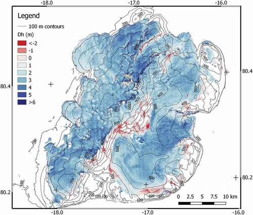
Figure 3. Elevation changes over the Holm Land Ice Cap as calculated from subtracting AeroDEM (1978) from ArcticDEM (2012–2015), using two different interpolation methods for void filling. Enlarged details show differences over void-filled areas

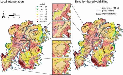
Consequently, over the course of 35 ±2 y from 1978 to 2012–2015, surface elevation has changed at an annual rate of −0.25 ±0.01 m a⁻¹ (elevation-based void filling) and −0.23 ±0.01 m a⁻¹ (local interpolation). Here, the uncertainty is estimated using error propagation of the random error in elevation change and in time (2 y). Figure 3 shows that the strongest ice loss is found in low-lying areas, especially at the glacier tongues in the southern sector. The higher elevations of the ice cap are dominated by surface lowering, but they reveal an inhomogeneous picture ranging from strong to moderate loss.

Elevation changes of individual glaciers range between −15.67 m and −4.22 m (see Table 4). Glaciers located in the southeast face stronger loss (RGI60-05.10000, RGI60-05.09998), whereas glaciers in the northeast reveal smaller elevation changes (RGI60-05.09994, RGI60-05.09992). No significant dependency between surface-elevation change and glacier area could be found.

Table 4. Individual elevation change at the ten major glaciers that cover 98 percent of the Holm Land Ice Cap and the respective random error

	Elevation Change (m)
Glacier	Elevation-Based Void Filling	Local Interpolation	Area (km^2)
RGI60-05.09992	−4.98 ±0.04	−6.40 ±0.04	141
RGI60-05.09993	−8.32 ±0.08	−9.77 ±0.08	38
RGI60-05.09994	−4.22 ±0.13	−5.55 ±0.13	14
RGI60-05.09995	−7.40 ±0.03	−8.64 ±0.03	215
RGI60-05.09996	−10.99 ±0.04	−12.44 ±0.04	153
RGI60-05.09997	−9.24 ±0.08	−10.67 ±0.08	39
RGI60-05.09998	−12.74 ±0.09	−14.02 ±0.09	26
RGI60-05.09999	−7.38 ±0.05	−8.75 ±0.05	112
RGI60-05.10000	−14.33 ±0.07	−15.67 ±0.07	43
RGI60-05.10001	−9.20 ±0.06	−10.71 ±0.06	68
Entire ice cap (mean of all twenty-five individual glaciers)	−8.56 ±0.02	−8.02 ±0.02	865

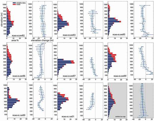
We averaged surface-elevation change over 100 m elevation bands and plotted the relationship of Δh to elevation z for individual glaciers (Figure 4) as well as for the entire ice cap (Figure 4, bottom-right panel). For the entire ice cap, loss in ice thickness is almost uniform with elevation. Standard deviation increases toward lower elevations because the glacier tongues show both thickening and thinning.

Figure 4. Hypsometry (from ArcticDEM) and the mean elevation change between AeroDEM (1978) and ArcticDEM (2012–2015) per 100 m elevation bins for the largest eight glaciers and the entire ice cap (bottom right, gray shading). Error bars indicate one standard deviation. For glacier numbering refer to Figure 1

The mean elevation changes of the two void-filling approaches differ by 0.55 m or 6 percent of the total elevation change (Table 3). Therefore, the elevation-based void filling suggests more loss than the local interpolation. When applying the elevation-based method, voids were filled using a relationship of Δh to elevation z calculated for each glacier individually. This has the advantage that differences in elevation change among the glaciers are considered, which are especially pronounced at lower elevations. However, most of the voids are located in the upper-most elevation bands that can contain up to 70–95 percent voids. Especially areas above ∼600 m a.s.l. are strongly affected. In order to increase the total number of valid data points in the upper elevation bands when applying the elevation-based void filling, a second calculation was performed where the relationship of Δh to z is based on the entire ice cap. The results of both calculations, however, differ only by 0.01 m a⁻¹.

Glacier length change (from 1978 to 2016)

Length changes inferred from comparing glacier extent as seen on the orthorectified photos from 1978 and on the Sentinel-2 image (2016) provide additional information. The majority of the large glaciers (seven out of ten) have retreated, but only by about 100–200 m, and their average surface elevation has decreased. An exception is the retreat by 1.2 km of the northwest-facing tongue of glacier RGI60-05.100001. Meanwhile, advances of glaciers differ from a few hundred meters (glacier RGI60-05.09993, glacier RGI60-05.09999) to more than 600 m (northern outlet of glacier RGI60-05.09995) and coincide with elevation gain. Glacier RGI60-05.09995 shows pronounced thinning just upstream from a thickening tongue (cf. Figure 3).

Differencing TanDEM-X and ArcticDEM

Subtracting TanDEM-X from ArcticDEM yields a mean elevation difference of 0.08 ±2.78 m over stable terrain and 2.54 ±1.40 m over the Holm Land Ice Cap (Figure 5). Because the ArcticDEM dates to 2012–2015 and the TanDEM-X to 2010–2014, their acquisition periods could overlap. The very small difference over stable terrain indicates that the two DEMs are virtually identical. The elevation difference over the ice cap, however, is clearly different from zero. Elevation difference is rather uniform and there is no clear relationship between surface-elevation difference and elevation. An exception is observed at glacier RGI60-05.09995, where a negative elevation difference upstream of the tongue is found, relative to the surrounding changes. This signature resembles the one that is present in the differentiated AeroDEM/ArcticDEM at the same location. Other pronounced features seen in the differentiated AeroDEM/ArcticDEM, such as the strong decrease in surface elevation at the tongues of the glaciers RGI60-05.10000 and RGI60-05.0999, cannot be found in the Δh of TanDEM-X and ArcticDEM (Figure 3).

Figure 5. Elevation differences over the Holm Land Ice Cap calculated from subtracting TanDEM-X (2010–2014) from ArcticDEM (2012–2015)

Elevation differences between ArcticDEM and TanDEM-X appear to be dependent on exposition. The values of Δh, adjusted for outliers and averaged over eight expositions, reveal that the south-facing slopes of the ice cap show lower elevation differences than the north-facing areas. The largest difference of 0.74 m is found between south-facing (mean 2.08 m) and northwest-facing slopes (mean 2.82 m). A two-tailed Student’s t-test using only valid pixels corrected for autocorrelation confirms that the difference is statistically significant. Calculations over stable terrain could not reproduce the same pattern.

Discussion

Uncertainties differentiating AeroDEM and ArcticDEM

Calculated standard errors of the elevation change between 1978 (AeroDEM) and 2012–2015 (ArcticDEM) quantifying random errors are small for both calculations of N_indp. The influence of systematic uncertainties, such as those resulting from the presence of data voids, is one order of magnitude larger. Because of the dominance of systematic errors, we provide a range of possible changes in surface elevation (between 1978 and 2012–2015) that covers both void filling methods. This range is given by –8.30 ± 0.28 m. Adding the random uncertainty (±0.02 m) yields to −8.30 ±0.30 m. Accordingly, mean surface-elevation changes at a rate of −0.24 ±0.02 m a⁻¹. The error of the surface-elevation change again quantifies a range and was estimated by error propagation of elevation and time uncertainty.

We identified both co-registration and void filling as main sources of systematic errors in mean elevation change. Co-registration suggests only subpixel shifts, but has an uncertainty in the same order of magnitude. This might be related to the lack of steep, high-elevation stable terrain in the study region that is required for optimal co-registration (Nuth and Kääb 2011).

Considering that 19 percent of the 1978 to 2012–2015 Δh grid of the Holm Land Ice Cap is subject to data voids, the influence of the choice of the two interpolation methods on the rates of surface-elevation change is small (−0.25 ±0.01 m a⁻¹ and −0.23 ±0.01 m a⁻¹, respectively). While the choice of interpolation has limited influence on the scale of the entire ice cap, prominent deviations occur on a local scale: Elevation-based void filling tends to create spurious artifacts when the function of Δh(z) is based on the entire ice cap (see enlarged details in Figure 3). These artifacts appear because the Δh(z) function for the entire ice cap differs from the functions for individual catchments (Figure 4). Better results are achieved by calculating and applying Δh(z) functions for individual catchments, but sudden changes in Δh still appear across borders between individual catchments.

When using only valid points and no interpolation at all (no void filling, Table 3) the result falls roughly halfway between the two void-filling approaches. Elevation-based void filling leads to a more negative result because the relationship of Δh to elevation z shows more loss in the higher elevation bands where most of the voids have to be filled. The local interpolation, however, suggests on the base of neighboring points that Δh over voids are more positive than the overall mean of the ice cap, indicating less loss in higher areas. It seems that the elevation-based void filling is not able to capture fine trends to more positive elevation changes around voids.

In the case of the Holm Land Ice Cap, void filling from local interpolation appears more suitable than elevation-based interpolation. This result, however, is not necessarily valid for other glacier types or spatial patterns of data voids. In the case of Holm Land, interpolation is facilitated by most data voids being surrounded by areas with reliable Δh data. Only on the western side of the ice cap do the uppermost elevations lack surrounding valid points. Where this problem is more widespread, for instance on valley-type glaciers with extended data voids bordering ice-free terrain (cf. Marcer et al. 2017) or swath-processed CryoSat-2 interferometric data with data voids being concentrated in the ablation areas (Foresta et al. 2016), local interpolation might result in spurious artifacts.

Restrictions when differentiating ArcticDEM and TanDEM-X

Over stable terrain, the average Δh between TanDEM-X and ArcticDEM is virtually zero, but glacier surfaces are lower by 2.54 ±1.40 m in TanDEM-X compared to ArcticDEM. The two DEMs have a very similar time stamp (Table 1), and in the TanDEM-X surface elevation resembles a weighted average of the overflights (Gruber et al. 2016). Considering this, the elevation difference over the ice cap appears too large to be explained by glacier mass balance alone. In relation to the 1978 to 2012–2015 surface-elevation change of −8.30 ±0.30 m, the average difference between the two DEMs is substantial. While we did not use TanDEM-X in the calculation of surface-elevation change from 1978 to 2012–2015, the example shows that DEM offsets established over stable terrain are not necessarily representative for glacier surfaces.

It appears less likely that the offset is caused by issues in the ArcticDEM, which would directly affect the accuracy of the calculated glacier thinning between 1978 and 2012–2015. Instead, the difference is likely related to the penetration of radar waves into snow and firn. Evidence for this assumption is given by the fact that south-facing slopes exhibit lower elevation differences. This might be related to more frequent melt on southern slopes, which leads to the presence of more ice in the glacier firn and reduces the penetration of X-band electromagnetic waves (cf. Nilsson et al. 2015). The SAR X-band signal penetration for TanDEM-X data (9.65 GHz) depends strongly on the water content of the snow. A study from the European Alps found a 4 m mean penetration depth at an elevation of 4,000 m a.s.l., with limited melting during the melt season (Dehecq et al. 2016). Similar conditions are found at the Antarctic margin, where penetration depths of 3.7–5.7 m were estimated (Groh et al. 2014). A physical model based on the water content of snow shows that penetration depths of the TanDEM-X radar signal can range between 69.4 m and 0.04 m, varying from dry, freshly fallen snow to wet snow with a liquid water content of 3 percent (Rossi et al. 2016). Therefore, the observed deviation might be related at least partly to the penetration of the X-band signal into the subsurface.

A second issue when interpreting Δh is the unknown time relation between ArcticDEM and TanDEM-X that might also be spatially inconsistent over the Holm Land Ice Cap. Certain changes, such as the thinning of glacier RGI60-05.09995, at high elevations are observed in both DEM pairs, others are reversed. Consequently, some parts of the signal likely reflect changes in ice thickness, but dating issues prevent us from a definitive interpretation.

Obviously, the calculation of shorter-term surface-elevation changes requires DEMs with precise time stamps. The TanDEM-X and ArcticDEM mosaics, with their blurred time stamps, have their strengths in application over longer time periods. However, our comparison of ArcticDEM and TanDEM-X mosaics shows a deviation over glacier surfaces that is large, even in the context of long-term glacier changes. These strong deviations between the two DEM products warrent further investigation as they point to error sources that are likely unrelated to the blurred time stamps.

Glacier thickness changes

To our knowledge, this is the first glaciological study focussing on the Holm Land Ice Cap. A study from Flade Isblink, which is the largest ice cap of the Greenland periphery (approximately 8,000 km²) and located only about 90 km north of Holm Land, reported mean elevation changes of 0.03 ±0.03 m a⁻¹, measured by EnviSAT (2002–2009), and 0.17 ±0.23 m a⁻¹, measured by ICESat (2004–2008; Rinne et al. 2011). Detailed spatial analysis reveals that although the western half of Flade Isblink thickened (0.5 m a⁻¹), the eastern half thinned at rates of up to 1 m a⁻¹, mainly in the lower ablation areas (Rinne et al. 2011).

Compared to Flade Isblink, average rates of ice-thickness loss on Holm Land are higher at −0.25 ±0.01 m a⁻¹ and −0.23 ±0.01 m a⁻¹, respectively. Thinning rates, however, are difficult to compare because our study covers a time period that is nearly ten times as long as the one offered by ICESat. Interestingly, Rinne et al. (2011) found a relatively consistent thickening in the interior of Flade Isblink, while we observe widespread thinning in the accumulation area of the Holm Land Ice Cap.

Marcer et al. (2017) studied surface-elevation change on a small (approximately 3 km²) glacier in southwest Greenland during a time period (1985–2014) similar to our study. Observed rates in surface-elevation change (−0.6 m a⁻¹) double the thinning rates determined for Holm Land. This is expected, because the glacier studied by Marcer et al. (2017) is located in a climatic setting that is warmer and moister. Such glaciers tend to react more sensitively to a given perturbation in climatic parameters, such as temperature and precipitation (e.g., Kuhn 1981; Oerlemans 1992).

Accounting for these regional differences, Bolch et al. (2013) divided Greenland into different regions to calculate mean elevation changes. For the central-north they found a mean change of −0.28 m a⁻¹ for land-terminating glaciers. Including marine-terminating glaciers, their elevation change decreased to −0.18 m a⁻¹, which is mainly caused by Flade Isblink, which shows almost no change in elevation. The mean annual change rate of the Holm Land Ice Cap falls between both values.

Using our estimated mean surface-elevation change for 1978 to 2012–2015, we obtain an ice-volume change at Holm Land of -7.18 ± 0.26 km³. When converted to mass change (assuming an average density of 850 ±60 kg m⁻³; cf. Huss 2013), this yields a mass loss of −6.1 ±0.5 Gt.

The change in glacier volume found by this study spans approximately thirty-five years and documents a long-term, climate-induced signal. Geodetic glacier-volume changes covering a climatological time period are relatively rare and especially valuable in the context of global glacier-change assessment (Zemp et al. 2015) Hence, the results feed well into the framework of other studies and add knowledge on the variability of mean elevation changes in Greenland. Furthermore, the high spatial resolution of the data sets allows the individual assessment of glaciers and could help identify surging glaciers. For example, glacier RGI60-05.09995 shows thinning upstream of a thickening tongue that might indicate surge-type behavior (e.g., Murray et al. 1998). So far, no surges on Holm Land have been reported (Sevestre and Benn 2015).

Conclusions

On the Holm Land Ice Cap, subtracting AeroDEM from ArcticDEM yielded an overall elevation change of −8.30 ±0.30 m for 1978 to 2012–2015. Covering approximately thirty-five years, the mean ice thinning of −0.24 ±0.02 m a⁻¹ represents a long-term signal and complements the results from other studies about Greenland’s peripheral glaciers. Besides mean rates of elevation changes for the whole ice cap, the changes in individual glaciers, including potential surge-type behavior, are well resolved. Consequently, AeroDEM and ArcticDEM provide a valuable source of information on the evolution of Greenland’s peripheral glaciers, with the following constraints:

• AeroDEM suffers from artifacts that can be masked out successfully using its reliability mask. In areas considered to be of optimal quality (such as the area of this study), data voids still make up 19 percent of all data. Additionally, AeroDEM suffers from local offsets on the order of a few meters that are not detected by its reliability mask and are difficult to correct.

• Co-registration suggests that there is, if any, only a subpixel shift between the three DEMs. However, the study area might not be optimally suited for co-registration based on Nuth and Kääb (2011), because there is a lack of steep, high-elevation stable terrain.

• The uncertainty originating from random errors is at least one order of magnitude smaller than systematic errors that are introduced by the interpolation method. Applying different void-filling techniques, we show that the spatial interpolation of the voids results in less negative estimates than the interpolation based on elevation gradients of Δh. The estimates differ by 0.55 m or 6 percent of the total elevation change.

Differencing ArcticDEM (2012–2015) and TanDEM-X (2010–2014) yields an elevation difference of 2.54 ±1.40 m, which probably reflects a mixed signal from penetration of the SAR X-band signal into snow and firn and actual ice-thickness loss. Uncertainties related to the unknown acquisition dates prevent additional interpretations.

Acknowledgments

We wish to thank K.K. Kjeldsen and A.A. Bjørk for valuable discussions of results and for help in assessing AeroDEM data quality as well as the related choice of our study region. Furthermore, we thank N. Mölg and P. Rastner for assistance in co-registration. The authors highly appreciate the constructive advice and input from two anonymous reviewers and the editors. The results on changes in glacier length and surface elevation are made available through the World Glacier Monitoring Service.

Disclosure statement

No potential conflict of interest was reported by the authors.

Additional information

Funding

This study is supported by the ESA project Glaciers_cci (40000109873/14/I-NB) and the Swiss GCOS Office at the Federal Office of Meteorology and Climatology MeteoSwiss.

References

- Bjørk, A. A., S. Aagaard, A. Lütt, S. A. Khan, J. E. Box, K. K. Kjeldsen, N. K. Larsen, N. J. Korsgaard, J. Cappelen, W. T. Colgan, et al. 2018. Changes in Greenland’s peripheral glaciers linked to the North Atlantic Oscillation. Nature Climate Change 8 (1):1–13. doi:https://doi.org/10.1038/s41558-017-0029-1.
- Bolch, T., L. S. Sørensen, S. Simonsen, N. Mölg, H. Machguth, P. Rastner, and F. Paul. 2013. Mass change of local glaciers and ice caps on Greenland derived from ICESat data. Geophysical Research Letters 40 (5):875–81. doi:https://doi.org/10.1002/grl.50270.
- Dehecq, A., R. Millan, E. Berthier, N. Gourmelen, E. Trouve, and V. Vionnet. 2016. Elevation changes inferred from TanDEM-X data over the Mont-Blanc area: Impact of the X-band interferometric bias. IEEE Journal of Selected Topics in Applied Earth Observations and Remote Sensing 9 (8):3870–82. doi:https://doi.org/10.1109/JSTARS.2016.2581482.
- Environmental Systems Research Institute (ESRI). 2017. ArcMap Help 10.6: Elevation void fill function. http://desktop.arcgis.com/en/arcmap/latest/manage-data/raster-and-images/elevation-void-fill-function.htm.
- Escher-Vetter, H., M. Kuhn, and M. Weber. 2009. Four decades of winter mass balance of Vernagtferner and Hintereisferner, Austria: Methodology and results. Annals of Glaciology 50 (50):87–95. doi:https://doi.org/10.3189/172756409787769672.
- Foresta, L., N. Gourmelen, F. Pálsson, P. Nienow, H. Björnsson, and A. Shepherd. 2016. Surface elevation change and mass balance of Icelandic ice caps derived from swath mode CryoSat-2 altimetry. Geophysical Research Letters 43:12138–45. doi:https://doi.org/10.1002/2016GL071485.
- Gardelle, J., E. Berthier, Y. Arnaud, and A. Kääb. 2013. Region-wide glacier mass balances over the Pamir-Karakoram-Himalaya during 1999–2011. The Cryosphere 7:1263–86. doi:https://doi.org/10.5194/tc-7-1263-2013.
- Groh, A., H. Ewert, R. Rosenau, E. Fagiolini, C. Gruber, D. Floricioiu, W. Abdel Jaber, S. Linow, F. Flechtner, M. Eineder, et al. 2014. Mass, volume and velocity of the Antarctic ice sheet: Present-day changes and error effects. Surveys in Geophysics 35 (6):1481–505. doi:https://doi.org/10.1007/s10712-014-9286-y.
- Gruber, A., B. Wessel, M. Martone, and A. Roth. 2016. The TanDEM-x DEM mosaicking: Fusion of multiple acquisitions using InSAR quality parameters. IEEE Journal of Selected Topics in Applied Earth Observations and Remote Sensing 9 (3):1047–57. doi:https://doi.org/10.1109/jstars.2015.2421879.
- Huss, M. 2013. Density assumptions for converting geodetic glacier volume change to mass change. The Cryosphere 7:877–87. doi:https://doi.org/10.5194/tc-7-877-2013.
- Korsgaard, N. J., C. Nuth, S. A. Khan, K. K. Kjeldsen, A. A. Bjørk, A. Schomacker, and K. H. Kjær. 2016. Digital elevation model and orthophotographs of Greenland based on aerial photographs from 1978–1987. Scientific Data 3:160032. doi:https://doi.org/10.1038/sdata.2016.32.
- Kuhn, M. 1981. Climate and glaciers. In Sea Level, Ice and Climatic Change, I. Allison (ed.), International Association of Hydrological Sciences, Publications No. 131, Wallingford, UK, pp. 3–20.
- Machguth, H., P. Rastner, T. Bolch, N. Mölg, L. S. Sørensen, G. Aalgeirsdottir, J. van Angelen, M. van den Broeke, and X. Fettweis. 2013. The future sea-level rise contribution of Greenland’s glaciers and ice caps. Environmental Research Letters 8 (8):025005. doi:https://doi.org/10.1088/1748-9326/8/2/025005.
- Machguth, H., H. Thomsen, A. Weidick, A. P. Ahlstrøm, J. Abermann, M. L. Andersen, S. Andersen, A. A. Bjørk, J. E. Box, R. J. Braithwaite, et al. 2016. Greenland surface mass balance observations from the ice sheet ablation area and local glaciers. Journal of Glaciology 62 (235):861–87. doi:https://doi.org/10.1017/jog.2016.75.
- Magnússon, E., J. M.-C. Belart, F. Pálsson, H. Ágústsson, and P. Crochet. 2016. Geodetic mass balance record with rigorous uncertainty estimates deduced from aerial photographs and lidar data – Case study from Drangajökull ice cap, NW Iceland. The Cryosphere 10 (1):159–77. doi:https://doi.org/10.5194/tc-10-159-2016.
- Marcer, M., P. Stentoft, E. Bjerre, E. Cimoli, A. Bjørk, L. Stenseng, and H. Machguth. 2017. Three decades of volume change of a small Greenlandic glacier using ground penetrating radar, structure from motion and aerial photogrammetry. Arctic, Antarctic, and Alpine Research 49 (3):411–25. doi:https://doi.org/10.1657/AAAR0016-049.
- McNabb, R. W., C. Nuth, and A. Kääb. 2017. Phase 2: Option 2, algorithm development: Voids. Technical Report. Glaciers_cci-D1.2_LAR, European Space Agency Glaciers CCI Project.
- Mernild, S. H., N. T. Knudsen, W. H. Lipscomb, J. C. Yde, J. K. Malmros, B. Hasholt, and B. H. Jakobsen. 2011. Increasing mass loss from Greenland’s Mittivakkat Gletscher. The Cryosphere 5:341–48. doi:https://doi.org/10.5194/tc-5-341-2011.
- Morin, P., C. Porter, M. Cloutier, I. M. Howat, M. J. Noh, M. Willis, B. Bates, C. Willamson, and K. Peterman. 2016. ArcticDEM. A publically available, high resolution elevation model of the Arctic. EGU General Assembly Conference Abstracts 811(18):8396.
- Murray, T., J. A. Dowdeswell, D. J. Drewry, and I. Frearson. 1998. Geometric evolution and ice dynamics during a surge of Bakaninbreen, Svalbard. Journal of Glaciology 44 (147):263–72. doi:https://doi.org/10.3189/s0022143000002604.
- Nilsson, J., P. Vallelonga, S. B. Simonsen, L. S. Sørensen, R. Forsberg, D. Dahl-Jensen, M. Hirabayashi, K. Goto-Azuma, C. S. Hvidberg, H. A. Kjær, et al. 2015. Greenland 2012 melt event effects on CryoSat-2 radar altimetry. Geophysical Research Letters 42:3919–26. doi:https://doi.org/10.1002/2015GL063296.
- Noël, B., W. J. van de Berg, S. Lhermitte, B. Wouters, H. Machguth, I. Howat, M. Citterio, G. Moholdt, J. T. M. Lenaerts, and M. R. van den Broeke. 2017. A tipping point in refreezing accelerates mass loss of Greenland’s glaciers and ice caps. Nature Communications 8:14730. doi:https://doi.org/10.1038/ncomms14730.
- Noh, M.-J., and I. M. Howat. 2015. Automated stereo-photogrammetric DEM generation at high latitudes: Surface extraction with TIN-based search-space minimization (SETSM) validation and demonstration over glaciated regions. GIScience & Remote Sensing 52 (2):198–217. doi:https://doi.org/10.1080/15481603.2015.1008621.
- Nuth, C., and A. Kääb. 2011. Co-registration and bias corrections of satellite elevation data sets for quantifying glacier thickness change. The Cryosphere 5:271–90. doi:https://doi.org/10.5194/tc-5-271-2011.
- Oerlemans, J. 1992. Climate sensitivity of glaciers in southern Norway: Application of an energy-balance model to Nigardsbreen, Hellstugubreen and Alfotbreen. Annals of Glaciology 38:223–32. doi:https://doi.org/10.1017/S0022143000003634.
- Pilgrim, L. 1996. Surface matching and difference detection without the aid of control points. Survey Review 33 (2):291–304. doi:https://doi.org/10.1179/sre.1996.33.259.291.
- Rastner, P., T. Bolch, N. Mölg, H. Machguth, R. Le Bris, and F. Paul. 2012. The first complete inventory of the local glaciers and ice caps on Greenland. The Cryosphere 6:1483–95. doi:https://doi.org/10.5194/tc-6-1483-2012.
- Reuter, H. I., A. Nelson, and A. Jarvis. 2007. An evaluation of void-filling interpolation methods for SRTM data. International Journal of Geographical Information Science 21 (9):983–1008. doi:https://doi.org/10.1080/13658810601169899.
- RGI Consortium. 2017. Randolph glacier inventory - A dataset of global glacier outlines: Version 6.0. Technical Report, Global Land Ice Measurements from Space, Colorado, USA. Digital Media. doi:https://doi.org/10.7265/N5-RGI-60.
- Rinne, E. J., A. Shepherd, S. Palmer, M. R. van den Broeke, A. Muir, J. Ettema, and D. Wingham. 2011. On the recent elevation changes at the Flade Isblink ice cap, northern Greenland. Journal of Geophysical Research 116:F03024. doi:https://doi.org/10.1029/2011JF001972.
- Rossi, C., C. Minet, T. Fritz, M. Eineder, and R. Bamler. 2016. Temporal monitoring of subglacial volcanoes with TanDEM-X — Application to the 2014–2015 eruption within the Bárðarbunga volcanic system, Iceland. Remote Sensing of Environment 181:186–97. doi:https://doi.org/10.1016/j.rse.2016.04.003.
- Sevestre, H., and D. I. Benn. 2015. Climatic and geometric controls on the global distribution of surge-type glaciers: Implications for a unifying model of surging. Journal of Glaciology 61 (228):646–62. doi:https://doi.org/10.3189/2015jog14j136.
- Wessel, B. 2016. TanDEM-X ground segment - DEM products specification document. Public Document TD-GS-PS-0021, Issue 3.1, EOC, DLR, Oberpfaffenhofen, Germany.
- Yde, J. C., K. Gillespie, R. Løland, H. Ruud, S. H. Mernild, S. De Villiers, N. T. Knudsen, and J. K. Malmros. 2014. Volume measurements of Mittivakkat Gletscher, southeast Greenland. Journal of Glaciology 60 (224):1199–207. doi:https://doi.org/10.3189/2014JoG14J047.
- Zemp, M., H. Frey, I. Gärtner-Roer, S. U. Nussbaumer, M. Hoelzle, F. Paul, W. Haeberli, F. Denzinger, P. A. Ahlstrøm, B. Anderson, et al. 2015. Historically unprecedented global glacier decline in the early 21st century. Journal of Glaciology 61 (228):745–62. doi:https://doi.org/10.3189/2015JoG15J017.