Hierarchical modeling of space-time dendroclimatic fields: Comparing a frequentist and a Bayesian approach

ABSTRACT

Environmental processes, including climatic impacts in cold regions, are typically acting at multiple spatial and temporal scales. Hierarchical models are a flexible statistical tool that allows for decomposing spatiotemporal processes in simpler components connected by conditional probabilistic relationships. This article reviews two hierarchical models that have been applied to tree-ring proxy records of climate to model their space–time structure: STEM (Spatio-Temporal Expectation Maximization) and BARCAST (Bayesian Algorithm for Reconstructing Climate Anomalies in Space and Time). Both models account for spatial and temporal autocorrelation by including latent spatiotemporal processes, and they both take into consideration measurement and model errors, while they differ in their inferential approach. STEM adopts the frequentist perspective, and its parameters are estimated through the expectation-maximization (EM) algorithm, with uncertainty assessed through bootstrap resampling. BARCAST is developed in the Bayesian framework, and relies on Markov chain Monte Carlo (MCMC) algorithms for sampling values from posterior probability distributions of interest. STEM also explicitly includes covariates in the process model definition. As hierarchical modeling keeps contributing to the analysis of complex ecological and environmental processes, proxy reconstructions are likely to improve, thereby providing better constraints on future climate change scenarios and their impacts over cold regions.

KEYWORDS:

• Tree rings
• STEM
• BARCAST
• climate reconstruction
• autocorrelation

Introduction

Ecological and environmental phenomena are usually complex, influenced by multiple interacting factors linked to physical and biological systems as well as anthropogenic influences. At the same time, in order to understand and manage the processes that control our environment, researchers and practitioners are finding opportunities and challenges in the growing availability of data from a wide range of sources with different spatial and temporal scales (Jin et al. 2015). In this framework, statistical research has been developed with the purpose of modeling complex phenomena by taking into account data and underlying (latent) sources of variability at multiple levels (Gelman 2006), and by providing results (e.g., parameter estimates, prediction maps, risk assessments) that explicitly quantify the corresponding degree of uncertainty. In particular, for studies on climate impacts (e.g., drought) and disturbance regimes (e.g., wildfires, insect outbreaks) at macrosystem scales (Heffernan et al. 2014; Becknell et al. 2015), investigators may combine instrumental data from monitoring networks or remote sensing, outputs from simulation models, and proxy data (e.g., tree-ring records; Harley et al. 2018). All these sources of information may differ in their spatial and temporal scales, measurement error, biases, and missing data; nevertheless, combining them using hierarchical, or completely nested, levels can lead to an improvement in analytical capability (Gelman and Hill 2006).

One of the most important environmental variables in cold regions is air temperature (Körner and Paulsen 2004; Paulsen and Körner 2014). While many different ways may exist to measure a variable such as temperature (Körner and Hiltbrunner 2018), in a strict sense it is impossible to measure, simulate, or reconstruct air temperature without errors. Instrumental observations from a set of sensors can be biased or missing if sensors are not properly calibrated or if they stop working. Monitoring or sampling sites are usually placed in locations that are not fully representative of the entire area of interest, a problem known as preferential sampling (for an air pollution example see Shaddick and Zidek 2014). When numerical outputs from simulation models are available, one should consider that deterministic models are a simplification of real complex systems found in nature; hence model errors should be taken into account. In tree-ring reconstructions of past air temperature changes, the final outcome may depend on data-processing choices made by the investigator. These choices include the screening of predictors to be used, the historical periods selected for model calibration and verification, the standardization formula used for obtaining the final tree-ring chronology, and so on. While progress continues to be made, for example, using signal-free (Melvin and Briffa 2008) and theory-based (Biondi and Qeadan 2008) standardization methods, other reconstruction issues, such as the universal use of the reverse regression method (Auffhammer et al. 2015), remain unresolved.

A statistical way to deal with most, if not all, of these issues consists in the definition of latent (or hidden) processes, also known as random effects, which represent the true state of a phenomenon (e.g., true air temperature) at the desired spatial and temporal resolution. Latent processes can be embedded inside hierarchical models, which are composed of multiple levels connected through conditional distributions. This is particularly useful when dealing with proxy climate reconstructions, which are notoriously plagued with difficulties (McShane and Wyner 2011), primarily because of the relatively low signal-to-noise ratio in the observations themselves (Hughes, Swetnam, and Diaz 2011; Bradley 2014).

Hierarchical (or multilevel) modeling is an active area of research (Clark and Gelfand 2006; Cressie and Wikle 2011), with applications in ecological, environmental, and epidemiological research (Cressie et al. 2009; Lawson 2009; Gelfand 2012). The capabilities of hierarchical models are primarily evident when massive amounts of data are available to represent complex, highly dimensional phenomena in space and time (Wikle 2003). Statistical approaches to climate reconstruction have also been recently framed in the flexible class of hierarchical models (Tingley et al. 2012). In fact, thanks to their conditional viewpoint, hierarchical models can manage complex processes by decomposing them in simpler components, while simultaneously considering uncertainty sources as well as spatial, temporal, and spatiotemporal interactions.

To navigate the increasing amount of scientific literature on hierarchical models, we offer here an introduction to tools that have been used for tree-ring reconstructions of climate, which are crucial to better constrain future scenarios on the impact of climatic changes, especially over cold regions. We introduce the basic notations of hierarchical modeling and spatial processes by describing and comparing two models that have been applied to tree-ring records in space and time: the STEM (spatiotemporal expectation maximization) model proposed by Fassó and Cameletti (2010) and the BARCAST (Bayesian algorithm for reconstructing climate anomalies in space and time) model developed by Tingley and Huybers (2010b). Characteristics, strengths, and limitations of the two models are discussed to highlight general differences in the frequentist and Bayesian approaches to hierarchical modeling. While the original STEM and BARCAST notations have been slightly modified for comparison reasons, we have attempted to strike a balance between a rigorous mathematical presentation and a desire to better inform interested scientists and practitioners about these powerful statistical tools.

Basic notions

Hierarchical modeling

At the first level of the hierarchy, the distribution¹ of the data Z = (Z₁,…, Z_n) is defined conditionally to the underlying latent processes Y = (Y₁,…, Y_n) and a set of parameters θ₁ that define the data model. This distribution, denoted by $\left[Z|Y,{\theta }_1\right]$, is known as likelihood. The second stage regards the distribution of all the hidden processes Y given other parameters contained in θ₂. The third level, which specifies the prior distribution of all the parameters θ = (θ₁, θ₂), is optional and exists only if we assume, as in the Bayesian approach, that parameters are random variables defined by a probability distribution. This hierarchical structure can be represented as follows (Wikle 2003):

Level 1—Data model: [data | processes, parameters] = [Z | Y, θ₁].

Level 2—Process model: [process | parameters] = [Y | θ₂].

Level 3—Parameter model (optional): [parameters] = [θ].

This can be also illustrated by means of the “directed acyclic graph” (DAG; Gelman et al. 2013; Figure 1), which is a structure consisting of nodes linked by unidirectional connections (a good example of a DAG is a family tree).

Figure 1. Directed acyclic graph (DAG) of a general hierarchical model structure, with data model given by [Z | Y, θ₁], process model by [Y | θ₂], and parameter prior model by [θ₁] and [θ₂]. Circles represent stochastic nodes, which may be observed, so that they are data, or unobserved, and therefore are latent processes; arrows denote stochastic dependence. Notice that arrows are unidirectional, and there is no cyclic pathway included in the graph.

If the modeling complexity increases, it is possible to decompose further each model into sublevels. For example, if two sets of data Z_a and Z_b are available, possibly with different spatiotemporal resolutions, two data models are specified conditional on the common process of interest Y and some parameters θ_1a, θ_1b. In this case the data model is usually defined for simplicity as

$\left[Z_a,Z_b|Y,{\theta }_{\text{1}a},{\theta }_{\text{1}b}\right]=\left[Z_a|Y,{\theta }_{\text{1}a}\right]\left[Z_b|Y,{\theta }_{\text{1}b}\right]$

meaning that, conditioned on the true process Y, the data are assumed to be independent, and thus the corresponding conditional distributions factorize.

The data and the process model can be combined in the following distribution:

(1) $\mathbf{[}Z,Y\left|\theta ]=[Z\right|Y,\theta ][Y|\theta ]=\left[Z|Y,{\theta }_1\right]\left[Y|{\theta }_2\right]$(1)

which represents the joint distribution of the data and the latent variables conditional upon the parameters. Statistical inference can then be carried out by means of a frequentist or a Bayesian approach. In the first case, parameters are considered fixed and unknown and can be estimated using a maximum likelihood (ML) procedure. In the case of hierarchical models with latent processes, one of the best ways to deal with the ML estimation is the expectation-maximization (EM) algorithm (McLachlan and Krishnan 1997). EM was originally proposed for ML estimation in presence of structural missing data (Dempster, Laird, and Rubin 1977), and its strength lies in not requiring to find the observed data likelihood. If the main interest is the estimation of the latent variable Y (e.g., the true temperature), the plug-in principle can be applied; that is, the ML parameter estimates are plugged into the conditional distribution [Y | θ]. This approach, however, does not take into account the parameter and spatial prediction uncertainty, a problem that can be solved, for example, through resampling procedures, such as the bootstrap (Efron and Tibshirani 1986).

The Bayesian approach assumes that the parameters are random variables with given prior distributions, which can incorporate experts’ opinions or results coming from previous studies (Gelman et al. 2013). The main interest of a Bayesian analysis is in the distribution of the unknown quantities given the data, that is, the posterior distribution, which is obtained through Bayes’ theorem and is given by

$\begin{array}{l}[Y,\theta |Z]=\frac{\left[Z,Y,\theta \right]}{\left[Z\right]}=\frac{\left[Z|Y,{\theta }_{\text{1}}\right]\left[Y|{\theta }_2\right]\left[\theta \right]}{\left[Z\right]}\\ \propto \left[Z|Y,{\theta }_1\right]Y|{\theta }_{\text{2}}\left[\theta \right]\end{array}$

where $\propto$ means “proportional to,” and the marginal distribution of the data [Z] in the denominator is a normalizing constant.

Samples from the posterior distribution may be simulated through Markov chain Monte Carlo (MCMC) algorithms (Brooks et al. 2011). The most used MCMC methods are the Gibbs sampler and the Metropolis–Hastings algorithm, which can be adapted to almost any kind of model, including hierarchical ones. A crucial aspect of MCMC concerns the computational costs, which can become prohibitive in case of massive data sets or complex models. Moreover, in order to get reliable and accurate MCMC outputs, attention has to be paid to the initial setting and tuning of the algorithm and to the convergence assessment. Recently, some new approaches have been proposed in the literature to speed up Bayesian estimation. Hamiltonian Monte Carlo (Girolami and Calderhead 2011; Neal 2011) is an algorithm, based on differential geometry, that is able to explore the density of the target distributions more efficiently than classical methods such as the Metropolis–Hastings one. It is implemented in the Stan software (http://mc-stan.org) and can result in improved efficiency and faster inference for complex problems in high-dimensional spaces. The integrated nested Laplace approximated (INLA, http://www.r-inla.org) method developed by Rue, Martino, and Chopin (2009) is a computationally effective alternative to MCMC designed for latent Gaussian models, which include a very wide and flexible class of hierarchical models ranging from (generalized) linear mixed models to spatiotemporal ones (Blangiardo and Cameletti 2015). Differently from the simulation-based MCMC methods, INLA is a deterministic algorithm that provides accurate and fast approximation of the posterior distributions.

Spatial processes

In many environmental studies, data are geographically referenced, meaning that each datum is associated with a location in space denoted by s. From a statistical point of view these spatial data are defined as realizations of a stochastic process (i.e., a collection of random variables) indexed by space, that is,

$Z(s)\equiv \left\{Z(s),s\in D\right\}$

where D is a (fixed) subset of a d-dimensional spatial domain. Following the classification adopted by Cressie (1993) and Gelfand et al. (2010), three types of spatial data have been identified:

• Area data: In this case Z(s) is a random aggregate value over an area unit s with well-defined boundaries in D, which is defined as a countable collection of areas. These data are often used in epidemiological mapping applications, where the observations may regard the number of deaths or hospitalizations in a given area, and the objective is estimating spatial risk related to a certain disease (Lawson 2009).

• Point-referenced (or geostatistical) data: In this case the spatial index s varies continuously in the fixed domain D, and Z(s) is a random outcome observed at a specific (nonrandom) location, which is typically a two-dimensional vector with latitude and longitude but may also include altitude. For example, we may be interested in air temperature for a specific region, a phenomenon that exists everywhere in the considered area but can be measured only at a limited number of monitoring stations with locations s₁,…, s_n.

• Spatial point patterns: In this case the locations are random and Z(s) represents the occurrence or not of an event—for example, coordinates of a given tree species in a forest or addresses of persons with a particular disease. In this case, while locations are random (e.g., we do not know a priori where trees will be located), Z(s) takes 0 or 1 values—that is, the event has occurred or not. If some additional covariate information is available (e.g., tree diameter), the point pattern process is marked (Illian et al. 2008).

In this article we consider the case of geostatistical data, assuming to deal with a phenomenon that changes continuously in a D subset of the two-dimensional space, but that is observed at a finite number of known locations. In the classical geostatistical model, Z(s) is defined as

$Z\left(s\right)=\mu (s)+e(s)$

where µ(s) is a mean also known as large-scale component, possibly defined as a polynomial trend surface or as a function of some covariates, and e(s) is a zero-mean stationary spatial process with covariance function Cov(e(s), e(s')). The spatial process is second-order stationary when the covariance function depends only on the separation vector h between locations for each s and s', and is isotropic when only the distance matters irrespective of direction (Cressie 1993). A commonly used covariance function is the exponential one, which is defined as

(2) $\mathrm{C}\mathrm{o}\mathrm{v}\left(e\left(s\right),e\left(s^{\prime }\right)\right)={\text{sigmaa}}^{2}exp\left(-\varphi h\right)={\text{sigmaa}}^2{C}_{\varphi }\left(h\right)$(2)

where h = ||s−s'|| is the Euclidean distance, σ² the spatial variance, and ϕ is related to the range R = 1/ϕ, defined as the distance at which the spatial covariance becomes almost null. Other covariance functions are available for defining isotropic second-order stationary spatial processes, and have been known for some time (see, e.g., Isaaks and Srivastava 1989).

Usually the main research interest in geostatistics is the prediction of the spatial process at new locations where it is not measured, a statistical procedure that is known as kriging. In the classical geostatistical approach (e.g., Diggle and Ribeiro 2007), the empirical variogram is used as an exploratory tool. In this preliminary stage, variogram models can sometime provide information by themselves on underlying ecological processes (Biondi, Myers, and Avery 1994). The mean and covariance parameters are estimated through least square methods, and a two-step procedure is usually adopted, whereby the mean is estimated first, and then residuals are used to make inference on the spatial parameters. Estimated parameters are plugged into the mean and covariance function, ignoring parameter uncertainty, and kriging is computed as a linear combination of the observed values. This approach provides nonoptimal estimators (Cressie and Wikle 2011); for this reason it is preferable to adopt a likelihood-based procedure like the ones adopted in the STEM and BARCAST models.

The concept of spatial process can be extended to the spatiotemporal case when spatial data are available at different times. A spatiotemporal random process (Wikle 2015) is simply a collection of random variables indexed by space and time, Z (s,t) ≡ $\left\{Z\left(s,t\right),\left(s,t\right)\right\}\in D$. In this case a valid (i.e., positive definite) spatiotemporal covariance function Cov(Z (s, t), Z (s', t')) should be defined. In practice, to overcome the computational complexity of spatio-temporal models, some simplifications are introduced. For example, it is possible to assume separability so that the space–time covariance function is decomposed into the sum (or the product) of a purely spatial and a purely temporal term. Alternatively, it can be supposed that the spatial correlation is constant in time, giving rise to a space-time covariance function that is purely spatial when t = t' and is zero otherwise. Temporal evolution could be introduced, assuming that the spatial process changes in time following autoregressive dynamics (Harvill 2010). This is the approach adopted by the STEM and BARCAST models, but we note briefly that another approach to take into account space–time covariance is by means of appropriate spatiotemporal variograms (Gneiting 2002).

Model analysis

STEM

STEM is a three-level hierarchical model implemented in the frequentist inferential framework through the EM algorithm. It was originally developed by Fassó and Cameletti (2010) for modeling air pollutant concentration, but it has been applied to hydroclimatological data sets, such as daily rainfall (Militino et al. 2015) and dendroclimatic records (Biondi 2014). For implementing the model, a software package named Stem (Cameletti 2013) is freely available in the R CRAN repository (R Core Team 2015).

Model description

Let the spatiotemporal process U(s, t) represent the true (latent) level of the considered phenomenon (e.g., air temperature), which is assumed to be observed with a measurement error at n monitoring stations and T time points. This yields, at the generic time t (t = 1,…, T), the following data model for the observations Z_t = (Z (s₁,t),…, Z (s_n,t)) coming from the n locations s₁,…,s_n:

(3) ${\mathit{Z}}_{\mathit{t}}=U_t+{\epsilon }_t$(3)

where ${\mathit{\epsilon }}_t$ is a multivariate zero mean normal distribution with independent and identically distributed (i.i.d.) components, that is, ${\epsilon }_t$ ∼ N(0, ${\text{sigmaa}}_{\text{varepsilonn}}^2$I_n), where ${\text{sigmaa}}_{\text{varepsilonn}}^2$ is the measurement error variance and I_n is an n-dimensional identity matrix. We then define Y_t = (Y₁ (t),…, Y_p (t)) as a p-dimensional vector (with p ≤ n) for the unobserved temporal process at time t (this could be related for example to the “true” air temperature). The process model is defined by the following two levels:

(4) ${\mathit{U}}_{\mathit{t}}=X_t\text{betaa}+K{Y}_t+{\omega }_t$(4)

(5) ${\mathit{Y}}_{\mathit{t}}=G{Y}_{t\mathit{-}1}+{\eta }_t$(5)

In equation (4) the unobserved spatio-temporal process U_t is defined as the sum of three components: a function of the (n × d)-dimensional matrix X_t defined by d covariates observed at time t at the n locations, the latent space-constant temporal process Y_t, and the spatiotemporal model error ω_t. The (n × p)-dimensional matrix K is known and accounts for the weights of the p components of Y_t for each spatial location s_i, i = 1,…,n. In equation (5) the temporal dynamics of Y_t are modeled as a p-dimensional autoregressive process of order 1, or AR(1), with G and η_t being the transition matrix and the innovation error, respectively. The three error components, namely, ε_t, η_t, and ω_t, have zero mean and are independent over time, as well as being mutually independent. In particular, η_t is supposed to follow a p-dimensional Gaussian distribution with variance–covariance matrix Σ_η. Finally, ω_t is an n-dimensional Gaussian spatial process for which the time-constant spatial covariance function is defined by the exponential covariance function in equation (2) with σ² = ${\text{sigmaa}}_{\omega }^2$; we also assume that Cov(η_t, ${\eta }_{t^{\prime }}$) = 0 for t ≠ t'.

Substitution of equation (4) into equation (3) yields the following two-stage hierarchical model:

(6) $Z_t=X_t\beta +K{Y}_t+e_t$(6)

(7) $Y_t=G{Y}_{t-1}+{\eta }_t$(7)

which has the structure of a state-space moddel (Durbin and Koopman 2001), with equations (6) and (7) representing the measurement equation and state equation, respectively. If all the parameters are known, the unobserved temporal process Y_t can be estimated for each time point t using the Kalman filter and Kalman smoother techniques (Wikle and Berliner 2007; Shumway and Stoffer 2011). The error e_t = ω_t + ε_t in equation (6) is uncorrelated in time, and for each time t has a zero-mean Gaussian distribution with variance–covariance matrix Σ_e for which the generic element is defined as follows:

(8) $\text{Cov}\left(e\left(s_i,t\right),e\left(s_j,t\right)\right)=\{\begin{array}{l}{\sigma }_{\omega }^2+{\sigma }_{\epsilon }^2{s}_i=s_j\left(h=0\right)\\ {\sigma }_{\omega }^2{C}_{\varphi }\left(h\right)s_i\ne s_j\left(h>0\right)\end{array}$(8)

The vector of unknown parameters of the STEM model is given by

(9) $\theta =\hspace{0.17em}\left\{\text{betaa},{\text{sigmaa}}_{\omega }^2,\mathit{G},{\mathbf{\Sigma }}_{\text{etaa}},\mathbf{log}\left(\mathit{\gamma }\right),\text{phii}\right\}$(9)

where log (γ) = log (${\text{sigmaa}}_{\epsilon }^2$/${\text{sigmaa}}_{\omega }^2$) is introduced for numerical purposes. Given the state-space model defined by equations (6) and (7), no conditions are required to ensure the positive definiteness of the variances in the models. In particular, as discussed in Sections 3.2 and 3.3 of Fassó and Cameletti (2009), it is possible to verify that the variances estimated using closed formulas are positive. The use of the logarithmic transformation for the positive definite parameter γ is related to the computational aspects of the Newton–Raphson (NR) algorithm, which is used to estimate γ (for which no closed formulas are available). Using log(γ) is therefore a computational requirement to avoid under- or over-flow when working with double-precision floating-point numbers. This helps with the convergence of the NR algorithm and to get a reasonable (i.e., positive definite) estimate of the parameter.

The log-likelihood function is

$\begin{array}{l}\log [Z|Y,]=\frac{-nT}{2}\log \left(2\pi \right)\\ -\frac{\text{1}}{2}{\displaystyle \sum _{t=1}^T\left(\log \left|{\Omega }_t\right|+{\left(Z_t-{\mu }_t\right)}^{\prime }{\Omega }_t^{-1}\left(Z_t{-}_t\right)\right)}\end{array}$

where ${\mathbf{\Omega }}_t=\left(\mathit{K}{P}_t^{t\mathit{-}1}{K}^{\prime }+{\mathbf{\Sigma }}_{\mathrm{e}}\right)$and ${\text{mua}}_{\mathbf{t}}=\left(X_t\text{betaa}+K{y}_t^{t\mathit{-}1}\right),$ with ${\mathit{y}}_t^{t-1}=E\left(Y\left(t\right)|Z_1,\dots ,Z_{t-1}\right)$ and ${\mathit{P}}_t^{t\mathit{-}1}=\mathrm{V}\mathrm{a}\mathrm{r}\left(Y\left(t\right)|Z_1,\dots ,Z_{t-1}\right)$ being the Kalman filter output, defined as the conditional mean and variance of Y_t given data up to time t−1. Such likelihood is a complex and nonlinear function of the unknown parameters, and its numerical maximization by means of classical Newton–Raphson algorithms (Gentle 2009) could be problematic. The adoption of the EM algorithm, which is described in the next section, copes with this problem.

Estimation with the EM algorithm

Maximum likelihood estimation of the unknown parameters in θ is performed by means of the EM algorithm (McLachlan and Krishnan 1997; Little and Rubin 2002), which is an iterative procedure especially useful for missing-data problems (Dempster, Laird, and Rubin 1977). Note that in the STEM model defined by equations (6) and (7), the missing-data component is given by the latent variable Y_t. The implementation of the EM algorithm for the STEM model (Fassó and Cameletti 2009, 2010) is briefly summarized in the following paragraph.

At each iteration k the EM algorithm alternates an expectation (E) and a maximization (M) step. Given the current values of the parameters θ ^(k), the E-step computes the expected value of the so-called complete likelihood function, defined as the joint distribution of the data Z and of the latent process Y = (Y₀,Y₁,…,Y_T) given the full observation matrix Z = (Z₁,…, Z_T) and θ^(k). This essentially corresponds to the joint distribution in equation (1) with θ = θ^(k). Then at the M-step the complete likelihood function is maximized with respect to θ, and the solution represents the updated parameter vector θ^(k+1). The EM algorithm converges when one or more criteria based on the distance between parameters are met; the ML estimates are then denoted by $\hat{\theta }$. For almost all parameters the M-step gives rise to closed-form solutions, which are very convenient from the computational point of view in terms of algorithm stability and reduced fast inference. Only for ϕ and log(γ) it is necessary to resort to numerical optimization methods, such as the Newton–Raphson algorithm, which represents an additional step inside each EM iteration. The main disadvantage of the EM algorithm is that it does not provide ready-to-use standard errors (i.e., uncertainty) of the parameter estimates. The available approaches for standard error estimation in the EM algorithm require the calculation of gradients, Hessian matrices, and conditional expected values, which can be really challenging to calculate, especially when the likelihood function is complex and involves recursive equations, as for the state-space model considered in this article. Thus, the bootstrap resampling method described in a later section represents a feasible approach for computing standard errors, and was adopted to overcome this problem.

Spatial prediction

The main purpose of geostatistical analysis is spatial prediction and mapping. Given the STEM model introduced earlier, the aim is estimating U(s₀,t) at a new spatial location s₀ given the actual data Z_t. The spatial predictor is obtained by the following joint (n + 1)-dimensional Gaussian conditional distribution:

$(\begin{array}{l}{Z}_t\\ U\left(s_0,t\right)\end{array}|Y_t,\theta )~N\left(\begin{array}{l}{\mu }_1\\ {\mu }_2\end{array}\right),\left(\begin{array}{cc}{\Sigma }_e& \Omega \\ {\Omega }^{\prime }& {\sigma }_{\omega }^2\end{array}\right)$

where ${\text{mua}}_{\mathit{1}}=X_t\text{betaa}+K{Y}_t$, ${\mu }_{\text{2}}=X\left(s_{\text{0}},t\right)\beta +K\left(s_{\text{0}}\right)Y_t$, and $X\left(s_{\text{0}},t\right)$ is the covariate vector observed at time t in the new site s₀. The quantity K($s_0$) is a p-dimensional loading vector. The covariance vector Ω is constant in time, and contains elements for i = 1,…,n given by

$\mathrm{C}\mathrm{o}\mathrm{v}\left[Z\left(s_i,t\right),U\left(s_0,t\right)\right]={\text{sigmaa}}_{\omega }^2\mathrm{e}\mathrm{x}\mathrm{p}\left(-\varphi ||s_i-s_0\right||).$

From multivariate Gaussian standard theory (Hoff 2009), it follows that the conditional random variable $U\left(s_0,t\right)|{\mathit{Z}}_t,{\mathit{Y}}_t,\theta$ has a univariate Gaussian distribution with mean $\hat{U}\left(s_0,t\right)$ and variance ${\widehat{\text{sigmaa}}}_K^2\left(s_0\right)$ given by

(10) $\widehat{U}\left(s_{\text{0}},t\right)={\mu }_2+{\Omega }^{\prime }{\Sigma }_e^{-1}{Z}_t-{\mu }_1$(10)

(11) ${\widehat{\text{sigmaa}}}_K^2\left(s_0\right)={\text{sigmaa}}_{\omega }^2-{\mathbf{\Omega }}^{\prime }{\mathbf{\Sigma }}_e^{-\mathit{1}}\mathbf{\Omega }$(11)

which coincide with the simple kriging predictor and error variance obtained in classical geostatistics (Cressie 1993).

Because the parameters θ and the latent process Y_t are unknown quantities, they are substituted, respectively, by the ML estimate $\hat{\theta }$ and by the Kalman smoother output. However, this solution does not take into account the uncertainty deriving from the parameter and latent process estimation. This could be overcome by substituting the kriging variance of equation (11) with an uncertainty measure that considers all sources of variability and is computed using the spatiotemporal bootstrap described in the next section.

Bootstrap for uncertainty assessment

The parametric bootstrap implemented by STEM is aimed at assessing the parameter and spatial prediction uncertainty. A number B of data samples are simulated from the Gaussian distributions of the STEM model. Equations (6) and (7), with parameter vector θ replaced by its ML estimate $\hat{\theta }$, are used to obtain a new data vector, while covariates are kept fixed for all simulations. A step-by-step description of the bootstrap simulation for each time t = 1,…,T is as follows:

• Simulate the random vector ${\mathit{\eta }}_t^{\ast }$ from the p-dimensional Gaussian distribution with zero mean and estimated variance-covariance matrix given by ${\hat{\mathbf{\Sigma }}}_{\text{etaa}}$.

• Use equation (7) to update the latent process, i.e. ${\mathit{Y}}_t^{\ast }=\hat{\mathit{G}}+{\mathit{K}Y}_{t\mathit{-}1}^{\ast }+{\mathit{\eta }}_t^{\ast }$.

• Simulate the random vector ${\mathit{e}}_t^{\ast }$ from the d-dimensional Gaussian distribution with zero mean and variance–covariance matrix given by ${\hat{\mathbf{\Sigma }}}_e$.

• Compute the bootstrap observation vector at time t as ${\mathit{Z}}_t^{\ast }={\mathit{X}}_t\widehat{\text{betaa}}+{\mathit{Y}}_t^{\ast }+{\mathit{e}}_t^{\ast }$.

• Obtain the b-th bootstrap sample Z^*_b = (Z^*₁,…, Z^*_T) by combining the simulated data for all the T times; note that the ML estimate ${\hat{\mathit{\theta }}}_b^{\ast }$ and the spatial prediction ${\hat{U}}_b^{\ast }\left(s_0,t\right)$ are computed using the EM algorithm and the kriging estimator previously described.

Repeating this procedure for b = 1,…,B produces the bootstrap replications ${\hat{\mathit{\theta }}}_1^{\ast },\dots ,{\hat{\mathit{\theta }}}_B^{\ast }$ and ${\hat{U}}_1^{\ast }\left(s_0,t\right),\dots ,{\hat{U}}_B^{\ast }\left(s_0,t\right)$, which are used for computing the standard error of each parameter and spatial prediction by simply calculating the sample variance. Percentile confidence intervals can be easily calculated from the empirical distributions; for example, the endpoints of the 95% percentile bootstrap confidence interval are given by the 2.5% and 97.5% quantiles of the bootstrap distribution.

BARCAST

The BARCAST model (Tingley and Huybers 2010a, 2010b) is implemented using a Bayesian approach. It was developed for the reconstruction of the temperature field by using both proxy and instrumental time series on a yearly basis. The model has been further used for other hydroclimatological studies (Tingley 2011; Werner, Luterbacher, and Smerdon 2012; Mannshardt, Craigmile, and Tingley 2013; Tingley and Huybers 2013), and the original Matlab code is freely available at ftp://ftp.ncdc.noaa.gov/pub/data/paleo/softlib/barcast.

Model description

In BARCAST the data model consists of two sublevels to take into account data from different sources. Let Z_I,t denote the instrumental (I) observations at time t, which are assumed to be the noisy versions of the true temperature, the latent process Y_I,t, according to the following model:

(12) ${\mathit{Z}}_{\mathit{I}\mathit{,}\mathit{t}}=Y_{I\mathit{,}t}+e_{I\mathit{,}t}$(12)

where e_I,t is the instrumental measurement error, assumed to be normally distributed with zero mean and variance equal to ${\text{sigmaa}}_I^2$ for each i.i.d. component. The second data model sublevel regards the proxy (P) observations Z_P,t, which are connected to the true temperature Y_P,t through a linear relationship given by

(13) ${\mathit{Z}}_{\mathit{P}\mathit{,}\mathit{t}}={\beta }_{\mathit{1}}{Y}_{P\mathit{,}t}+{\beta }_0\mathbf{1}+e_{P\mathit{,}t}$(13)

where 1 is a vector of ones for the intercept β₀, and the noise term e_P,t is given by i.i.d. normal distributions, each being distributed as N(0, ${\text{sigmaa}}_P^2$).

The process model defines the distribution of the true temperature process at the instrumental and proxy, and for the full vector Y = (Y_I,t, Y_P,t) it is defined by a multivariate AR(1) process given by

(14) ${\mathit{Y}}_{\mathit{t}}-\mu \mathbf{1}=\alpha \left(Y_{t\mathit{-}\mathit{1}}-\mu \mathbf{1}\right)+{\omega }_t$(14)

where $\alpha$ is the autoregressive coefficient, and the innovations ω_t are assumed to be independent in time and spatially dependent, with distribution given by ω_t ~ N(0, Σ_ω). The generic element of Σ_ω is given by the exponential spatial covariance function of equation (2) with ${\text{sigmaa}}^2={\text{sigmaa}}_{\omega }^2$.

As BARCAST adopts the Bayesian approach (e.g., Gelman et al. 2013), there is an additional, third level for the specification of the prior distributions, the so-called parameter model. Weakly informative but proper priors are specified for the eight parameters contained in θ = (θ₁, θ₂), where ${\theta }_{\text{1}}=\left({\sigma }_I^{\text{2}},{\sigma }_P^{\text{2}},\mu ,{\beta }_{\text{0}},{\beta }_{\text{1}}\right)$ and ${\theta }_2=\left({\text{sigmaa}}_{\omega }^2,\varphi ,\alpha \right)$. In particular, as specified in Table 1 and Appendix A of Tingley and Huybers (2010b), the following prior distributions are used in BARCAST: inverse-gamma for the variances; normal for $\mu ,{\beta }_0,\mathrm{a}\mathrm{n}\mathrm{d}{\beta }_1$; uniform for $\alpha$; and log-normal for $\varphi$. The hyperparameters of these distributions are chosen in order to obtain proper but weakly informative priors and to have the posterior distributions dominated by the data. For example, the interval [0,1] is chosen as support of the uniform distribution used for the coefficient $\alpha$ of the stationary AR(1) model of equation (14). This is a reasonable choice when the temporal correlation is expected to be positive, but the preferred prior should not be too informative. Another example can be provided for the inverse range parameter $\varphi$, for which the hyperparameters of the log-normal distribution are chosen by assuming that spatial correlation is present at distances between 10 and 1000 km, as is appropriate for large-scale climate reconstructions.

Given the model defined by equations (12)–(14), the joint posterior distribution of the parameters and latent process is given by

(15) $\begin{array}{l}\left[Y_{\text{0}},\dots ,Y_T,\theta |Z_{\text{1}},\dots ,Z_T\right]\\ \propto \left[Y_{\text{0}}\right]\theta \prod _{t=\text{1}}^T[Z_t|Y_t,{\theta }_{\text{1}}][Y_t|Y_{\text{t-1}},{\theta }_{\text{2}}]\end{array}$(15)

which corresponds to the complete-likelihood function of the STEM model.

Bayesian estimation

Parameter estimation is implemented via MCMC methods, which produce replicates drawn from the posterior distribution of equation (15). In practice, given m MCMC iterations indexed by l, for the generic parameter θ_i in θ, the set of values $\left\{{\text{thetaa}}_i^{\left(l\right)},l=l_0+1,\dots ,m\right\}$ simulated from the corresponding posterior distribution is available, where l₀ is the number of iterations discarded in order to eliminate the starting values influence (also known as the “burn-in period”). This set can be used to compute relevant posterior summaries (e.g., mean, median) or a measure of uncertainty given by the sample variance; moreover, a 95% credible interval can be immediately derived by using the 2.5% and 97.5% quantiles.

For all parameters but ϕ, which is the inverse of the spatial range, BARCAST employs the Gibbs sampler (Casella and George 1992). This method is appropriate when the full conditional distribution, that is, the posterior conditional distribution of a parameter given all unknown quantities, is a known distribution from which it is easy to sample. Such a condition is usually satisfied when Gaussian distributions are combined with conjugate priors—in Bayesian terms, a prior is conjugate to a given likelihood when the posterior distribution belongs to the same family as the prior distribution (Hoff 2009). The Gibbs sampling fails for ϕ because the full conditional is intractable, and hence the Metropolis–Hastings algorithm (Chib and Greenberg 1995) is used. This hybrid MCMC method has also been called the Metropolis-within-Gibbs algorithm (Banerjee, Carlin, and Gelfand 2014), and it operates by individually updating the parameters at each MCMC iteration.

Spatial prediction

In the Bayesian framework, to estimate at time t the true temperature at a new location s₀, it is not necessary to adopt the plug-in approach used by STEM. This is due to the fact that the posterior predictive distribution, which is the basis for Bayesian prediction, naturally includes parameter uncertainty. Thus, it is possible to write

(16) $\left[Y\left(s_0,t\right)|\mathit{Z}\right]=\int \left[Y\left(s_0,t\right),\mathit{\theta }|\mathit{Z}\right]\mathrm{d}\theta =\int \left[Y\left(s_0,t\right)|\mathit{\theta }\mathbf{,}\mathit{Z}\right][\mathit{\theta }|\mathit{Z}]\mathrm{d}\mathit{\theta }$(16)

where [Y (s₀) | θ, Z] has a conditional normal distribution obtained from the joint multivariate Gaussian distribution of Y(s₀, t). In practice, values from [Y (s₀) | Z] can be obtained through composition sampling (Banerjee, Carlin, and Gelfand 2014) using posterior draws of the parameters θ. This consists of using each value in the set $\left\{{\theta }^{\left(k\right)},k=k_0+1,\dots ,m\right\}$, which is obtained from the posterior [θ | Z] as described in the previous section, to simulate a value Y(s₀,t)^(k) from [Y(s₀)|θ, Z] with θ = θ^(k). Then the collection $\left\{Y{\left(s_0,t\right)}^{\left(k\right)},k=k_0+1,\dots ,m\right\}$ forms a sample from the posterior predictive distribution, and can be used to compute posterior summaries such as the median, variance, credible quantile intervals, and the likelihood of exceeding a given threshold.

Discussion

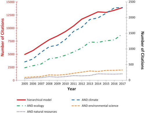
Statistics has a key role in the scientific understanding of environmental and ecological dynamics, because it can model possible sources of variability and provide a probabilistic evaluation of estimates and predictions (Katz 2002; Katz et al. 2013). Not surprisingly, the number of citations for hierarchical modeling in ecology and climate research has increased rapidly in recent years, even outpacing the rate of growth of citations for hierarchical models in general (Figure 2). Understanding past climate variability is crucial for placing accurate constraints on current and potentially future changes, despite the difficulties involved in properly using proxy records for climate reconstructions (National Research Council 2006). In this article, we have used formal mathematical notation to explain similarities and differences between two hierarchical space–time models for tree-ring reconstructions of climate, with one providing an example of a frequentist approach (STEM), and the other having a Bayesian character (BARCAST).

Figure 2. Publications listed by Google Scholar (https://scholar.google.com) over the past years (2005–2017). Search terms were “hierarchical model” either alone (plotted on the left y-axis) or together (logical AND) with the discipline (“ecology,” “climate,” “environmental science,” “natural resource”; all plotted on the right y-axis). The number of citations for hierarchical models almost tripled (a 2.8-fold increase) during the past 13 years, but that overall growth was exceeded by their applications in all fields: environmental science (3.6-fold increase), ecology (3.7-fold increase), climate (4.0-fold increase), and natural resources (4.2-fold increase).

There are also nonhierarchical models that have been used and described in the literature to reconstruct climate fields from proxy records, such as the regularized EM (RegEM) algorithm for Gaussian data (Schneider 2001). This approach is based on iterated multivariate linear regression analysis of variables (e.g., air temperature) with missing values on variables with available values (e.g., tree-ring proxy data), also accounting nonparametrically for spatial and temporal (auto)correlation. More recently, Guillot, Rajaratnam, and Emile-Geay (2015) proposed an extension of RegEM called the GraphEM method, which combines the EM algorithm with a Gaussian Markov random field for modeling the spatial temperature field through a neighborhood-graph approach. The hierarchical model structure has been again adopted by Tipton et al. (2016), who proposed a Bayesian model for tree-ring data based on a mixture of Gaussian distributions that depend on two deterministic growth models defined as a function of climate data (temperature and precipitation). The model has been applied to multiple tree species and is able to deal with the temporal misalignment given by the fact that climate data have a monthly resolution while tree-ring data are annual. Both temporal and spatial (auto)correlation are introduced parametrically by means of a temporal multivariate conditionally autoregressive structure (Cressie and Wikle 2011).

It is always a challenge to bridge the gap between advanced statistical methods and traditional applications of well-established procedures, especially because of the relatively fast pace of current advances. For instance, Bayesian hierarchical models have recently been used to reconstruct temperature by jointly modeling tree-ring width, age, and climate data (Schofield et al. 2016). This joint modeling approach is an alternative to the multistep conventional methodologies for reconstructing a climate variable, such as the traditional standardization and generation of tree-ring chronologies followed by climate reconstruction (Fritts 1976). Besides overcoming the “segment length curse” (Cook et al. 1995), the joint modeling approach is able to propagate the parameter estimation uncertainty from the standardization through the reconstruction. Using the same set of data (i.e., the Torneträsk ring-width data) used by Schofield et al. (2016), first Steinschneider et al. (2017) and then Schofield and Barker (2017) investigated the predictive performance of several modeling choices, including data transformation, inclusion of temporal autocorrelation, and homogenous or heterogeneous variance. However, none of these recent modeling efforts took explicitly into account spatial (auto)correlation.

With regard to model structure, STEM and BARCAST both include spatial and temporal components. In particular, STEM includes a process model—equation (4)—that comprises a linear function of covariates, a spatial process uncorrelated in time, and a low-dimensional temporal process with AR(1) dynamics. BARCAST has a two-level data model for taking into account both instrumental and proxy time series, each having a different relationship with the latent temporal field. The BARCAST process model—equation (14)—is characterized by an AR(1) temporal structure with spatially correlated and serially independent innovations. The size of the AR(1) latent process is defined by the number of spatial sites n for BARCAST, while for STEM it is given by p ≤ n, where p can be determined from the observed data using a principal component decomposition (Wikle and Cressie 1999) or can be set equal to one (Cameletti, Ignaccolo, and Bande 2011). It should be mentioned that tree growth may have time-series persistence that extends well beyond one year, but first-order autoregressive models have usually performed well for prewhitening tree-ring chronologies of the western United States (Biondi and Swetnam 1987).

Despite differences in hierarchical structure, both models are quite flexible. The inclusion of covariates, such as individual- and site-level variables that can account for confounding factors, is straightforward in STEM thanks to the measurement equation (6). An example of such covariates is site elevation, which can play a critical role in the identification of dendroclimatic signals across an entire tree-ring network (Touchan et al. 2016). In BARCAST it is possible to include additional variables in the process model (14), even though they would not be spatially explicit. With regard to the inferential approach, STEM estimation is performed via EM algorithm in a frequentist approach, assuming that parameters are fixed and unknown, whereas BARCAST has a Bayesian perspective that calls for parameter prior distributions. This means that assessing the uncertainty of parameter estimates and spatial predictions is straightforward for BARCAST (just by computing summaries of the posterior draws), while STEM requires a two-step procedure involving bootstrap as a resampling method. Both approaches are viable and effective for estimating hierarchical models, and it is not a priori possible to determine which method is preferable in terms of computational requirements or accuracy of results. Although different in hierarchical structure and inferential aspects, both models take advantage of the conditional viewpoint when dealing with probability distributions. Moreover, if all scalar parameters are not considered as random variables but are specified a priori, the BARCAST estimates of the latent field Y are equivalent to those from the Kalman smoother method adopted by STEM (Tingley and Huybers 2010b). This provides an interesting connection between the frequentist and the Bayesian philosophy.

From the computational point of view, both STEM and BARCAST cannot be implemented using ready-to-use software, but ad hoc code has been made freely available by the model authors. The computational effort required by the two models is likely to be similar, as both are based on iterative methods: STEM makes use of the EM algorithm for each bootstrap iteration, while BARCAST alternates the Gibbs and the Metropolis–Hastings algorithms at each MCMC iteration. For both STEM and BARCAST, it is possible to reduce the processing time by exploiting parallel computing, that is, by splitting a computation-intensive problem into smaller jobs to be solved concurrently by a cluster of processors or central processing unit (CPU) cores (Fassó and Cameletti 2009; Tingley and Huybers 2010b).

STEM and BARCAST have both been extended. BARCAST has inspired several spatiotemporal hierarchical models for hydroclimatological reconstruction (Tingley et al. 2012), and its capability to preserve the temporal persistence of long-range memory in simulated data has been recently tested by Nilsen et al. (2018). A new version of STEM named D-STEM (Distributed Space Time Expectation Maximization) has been proposed for the analysis of multivariate space–time data, such as those generated by the fusion of ground-level and remote-sensing observations (Fassó and Finazzi 2011). A model very similar to STEM has been applied to air pollution data (Cameletti et al. 2013) in a Bayesian context by means of the INLA algorithm (Blangiardo et al. 2013; Blangiardo and Cameletti 2015). As hierarchical modeling, either with a frequentist or a Bayesian approach, keeps contributing to the analysis of complex ecological and environmental processes in space and time, proxy reconstructions of climate will continue to improve, thereby providing better constraints on future climate change scenarios and their impacts over cold regions.

Disclosure statement

No potential conflict of interest was reported by the authors.

Additional information

Funding

M.C. was supported by the PRIN EphaStat Project (project 20154X8K23, https://sites.google.com/site/ephastat) provided by the Italian Ministry for Education, University and Research. F.B. was supported, in part, by the U.S. National Science Foundation under grants AGS-P2C2-1401381 and AGS-P2C2-1502379. The views and conclusions contained in this document are those of the authors and should not be interpreted as representing the opinions or policies of the funding agencies.

Notes

1. Following Gelfand and Smith (1990), brackets denote probability density functions of random variables. For example, [X] is the marginal distribution of the unidimensional random variable X, while [X |Y] and [X,Y] represent the conditional and joint distribution of X and Y, respectively. Bold characters are adopted for multivariate random variables.

References

- Auffhammer, M., B. Li, B. Wright, and S.-J. Yoo. 2015. Specification and estimation of the transfer function in dendroclimatological reconstructions. Environmental and Ecological Statistics 22 (1):105–26. doi:10.1007/s10651-014-0291-6.
- Banerjee, S., B. P. Carlin, and A. E. Gelfand. 2014. Hierarchical modeling and analysis for spatial data. 2nd ed. New York, New York, USA: Chapman and Hall.
- Becknell, J. M., A. R. Desai, M. C. Dietze, C. A. Schultz, G. Starr, P. A. Duffy, J. F. Franklin, A. Pourmokhtarian, J. Hall, P. C. Stoy, et al. 2015. Assessing interactions among changing climate, management, and disturbance in forests: A macrosystems approach. Bioscience 65 (3):263–74. doi:10.1093/biosci/biu234.
- Biondi, F. 2014. Dendroclimatic reconstruction at km-scale grid points: A case study from the Great Basin of North America. Journal of Hydrometeorology 15 (2):891–906. doi:10.1175/JHM-D-13-0151.1.
- Biondi, F., D. E. Myers, and C. C. Avery. 1994. Geostatistically modeling stem size and increment in an old-growth forest. Canadian Journal of Forest Research 24 (7):1354–68. doi:10.1139/x94-176.
- Biondi, F., and F. Qeadan. 2008. A theory-driven approach to tree-ring standardization: Definining the biological trend from expected basal area increment. Tree-Ring Research 64 (2):81–96. doi:10.3959/2008-6.1.
- Biondi, F., and T. W. Swetnam. 1987. Box-Jenkins models of forest interior tree-ring chronologies. Tree-Ring Bulletin 47:71–95.
- Blangiardo, M., and M. Cameletti. 2015. Spatial and Spatio-temporal Bayesian Models with R - INLA, 308. Chichester, West Sussex, UK: John Wiley & Sons.
- Blangiardo, M., M. Cameletti, G. Baio, and H. Rue. 2013. Spatial and spatio-temporal models with R-INLA. Spatial and Spatio-Temporal Epidemiology 4:33–49.
- Bradley, R. S. 2014. Paleoclimatology, 696. 3rd ed. San Diego, California, USA: Academic Press.
- Brooks, S., A. Gelman, G. L. Jones, and X.-L. Meng. 2011. Handbook of Markov Chain Monte Carlo, 619. Boca Raton, FL: CRC Press, Taylor & Francis Group.
- Cameletti, M. 2013. Package ‘Stem’: Spatio-temporal models in R, 17. R Foundation for Statistical Computing. https://cran.r-project.org/web/packages/Stem/Stem.pdf.
- Cameletti, M., F. Lindgren, D. Simpson, and H. Rue. 2013. Spatio-temporal modeling of particulate matter concentration through the SPDE approach. AStA Advances in Statistical Analysis 97 (2):109–31. doi:10.1007/s10182-012-0196-3.
- Cameletti, M., R. Ignaccolo, and S. Bande. 2011. Comparing spatio-temporal models for particulate matter in Piemonte. Environmetrics 22 (8):985–96. doi:10.1002/env.v22.8.
- Casella, G., and E. George. 1992. Explaining the Gibbs sampler. The American Statistician 46:167–74.
- Chib, S., and E. Greenberg. 1995. Understanding the Metropolis-Hastings algorithm. The American Statistician 49:327–35.
- Clark, J. S., and A. E. Gelfand. 2006. Hierarchical modeling for the environmental sciences: Statistical methods and applications, 216. New York, USA: Oxford University Press.
- Cook, E. R., K. R. Briffa, D. M. Meko, D. A. Graybill, and G. S. Funkhouser. 1995. The ‘segment length curse’ in long tree-ring chronology development for palaeoclimatic studies. The Holocene 5 (2):229–37. doi:10.1177/095968369500500211.
- Cressie, N. A. C. 1993. Statistics for spatial data, 900. Rev ed. New York: Wiley-Interscience.
- Cressie, N. A. C., C. A. Calder, J. S. Clark, J. M. V. Hoef, and C. K. Wikle. 2009. Accounting for uncertainty in ecological analysis: The strengths and limitations of hierarchical statistical modeling. Ecological Applications 19 (3):553–70.
- Cressie, N. A. C., and C. K. Wikle. 2011. Statistics for spatio-temporal data, 624. Hoboken, NJ: Wiley.
- Dempster, A. P., N. M. Laird, and D. B. Rubin. 1977. Maximum likelihood from incomplete data via the EM algorithm. Journal of the Royal Statistical Society. Series B (Methodological) 39 (1):1–38. doi:10.1111/j.2517-6161.1977.tb01600.x.
- Diggle, P. J., and P. J. Ribeiro. 2007. Model based geostatistics. New York, New York, USA: Springer.
- Durbin, J., and S. Koopman. 2001. Time series analysis by state space methods. New York, New York, USA: Oxford University Press.
- Efron, B., and R. J. Tibshirani. 1986. Bootstrap methods for standard errors, confidence intervals, and other measures of statistical accuracy. Statistical Science 1 (1):54–75. doi:10.1214/ss/1177013815.
- Fassó, A., and F. Finazzi. 2011. Maximum likelihood estimation of the dynamic coregionalization model with heterotopic data. Environmetrics 22 (6):735–48. doi:10.1002/env.1123.
- Fassó, A., and M. Cameletti. 2009. The EM algorithm in a distributed computing environment for modelling environmental space-time data. Environmental Modelling & Software 24:1027–35.
- Fassó, A., and M. Cameletti. 2010. A unified statistical approach for simulation, modeling, analysis and mapping of environmental data. Simulation 86 (3):139–54. doi:10.1177/0037549709102150.
- Fritts, H. C. 1976. Tree rings and climate, 567. London, UK: Academic Press.
- Gelfand, A. E. 2012. Hierarchical modeling for spatial data problems. Spatial Statistics 1:30–39.
- Gelfand, A. E., and A. F. M. Smith. 1990. Sampling-based approaches to calculating marginal densities. Journal of the American Statistical Association 85 (410):398–409. doi:10.1080/01621459.1990.10476213.
- Gelfand, A. E., P. J. Diggle, M. Fuentes, and P. Guttorp. 2010. Handbook of spatial statistics.
- Gelman, A. 2006. Multilevel (hierarchical) modeling: What it can and cannot do. Technometrics 48 (3):432–35. doi:10.1198/004017005000000661.
- Gelman, A., J. Carlin, H. Stern, D. Dunson, A. Vehtari, and D. B. Rubin. 2013. Bayesian data analysis, 675. Boca Raton, FL: CRC Press, Taylor & Francis Group.
- Gelman, A., and J. Hill. 2006. Data analysis using regression and multilevel/hierarchical models. Cambridge: Cambridge University Press.
- Gentle, J. E. 2009. Computational statistics, 728. New York, NY: Springer.
- Girolami, M., and B. Calderhead. 2011. Riemann manifold Langevin and Hamiltonian Monte Carlo methods. Journal of the Royal Statistical Society: Series B (Statistical Methodology) 73 (2):123–214. doi:10.1111/rssb.2011.73.issue-2.
- Gneiting, T. 2002. Nonseparable, stationary covariance functions for space-time data. Journal of the American Statistical Association 97 (458):590–600. doi:10.1198/016214502760047113.
- Guillot, D., B. Rajaratnam, and J. Emile-Geay. 2015. Statistical paleoclimate reconstructions via Markov random fields. The Annals of Applied Statistics 9 (1):324–52. doi:10.1214/14-AOAS794.
- Harley, G., C. Baisan, P. Brown, D. Falk, W. Flatley, H. Grissino-Mayer, A. Hessl, E. Heyerdahl, M. Kaye, C. Lafon, et al. 2018. Advancing dendrochronological studies of fire in the United States. Fire 1 (1):art.11 (16 pp.). doi:10.3390/fire1010011.
- Harvill, J. L. 2010. Spatio-temporal processes. Wiley Interdisciplinary Reviews: Computational Statistics 2 (3):375–82. doi:10.1002/wics.88.
- Heffernan, J. B., P. A. Soranno, M. J. Angilletta, L. B. Buckley, D. S. Gruner, T. H. Keitt, J. R. Kellner, J. S. Kominoski, A. V. Rocha, J. Xiao, et al. 2014. Macrosystems ecology: Understanding ecological patterns and processes at continental scales. Frontiers in Ecology and the Environment 12 (1):5–14. doi:10.1890/130017.
- Hoff, P. 2009. A first course in Bayesian statistical methods, 271. New York, NY: Springer.
- Hughes, M. K., T. W. Swetnam, and H. F. Diaz. 2011. Dendroclimatology: Progress and prospects, 365. Dordrecht: Springer Science+Business Media B.V.
- Illian, J., A. Penttinen, H. Stoyan, and D. Stoyan. 2008. Statistical analysis and modelling of spatial point patterns, 536. Chichester: Wiley.
- Isaaks, E. H., and R. M. Srivastava. 1989. An introduction to applied geostatistics. New York: Oxford University Press.
- Jin, X., B. W. Wah, X. Cheng, and Y. Wang. 2015. Significance and challenges of big data research. Big Data Research 2 (2):59–64. doi:10.1016/j.bdr.2015.01.006.
- Katz, R. W. 2002. Techniques for estimating uncertainty in climate change scenarios and impact studies. Climate Research 20 (2):167–85. doi:10.3354/cr020167.
- Katz, R. W., P. F. Craigmile, P. Guttorp, M. Haran, B. Sanso, and M. L. Stein. 2013. Uncertainty analysis in climate change assessments. Nature Climate Change 3 (9):769–71. doi:10.1038/nclimate1980.
- Körner, C., and E. Hiltbrunner. 2018. The 90 ways to describe plant temperature. Perspectives in Plant Ecology, Evolution and Systematics 30:16–21.
- Körner, C., and J. Paulsen. 2004. A world-wide study of high altitude treeline temperatures. Journal of Biogeography 31:713–32.
- Lawson, A. B. 2009. Bayesian disease mapping: Hierarchical modeling in spatial epidemiology, 464. Boca Raton, FL: CRC Press, Taylor & Francis Group.
- Little, R. J. A., and D. B. Rubin. 2002. Statistical analysis with missing data, 392. 2nd ed. Hoboken, New Jersey, USA: John Wiley & Sons.
- Mannshardt, E., P. F. Craigmile, and M. P. Tingley. 2013. Statistical modeling of extreme value behavior in North American tree-ring density series. Climatic Change 117 (4):843–58. doi:10.1007/s10584-012-0575-5.
- McLachlan, G. J., and T. Krishnan. 1997. The EM algorithm and extensions. New York, New York, USA: Wiley.
- McShane, B. B., and A. J. Wyner. 2011. A statistical analysis of multiple temperature proxies: Are reconstructions of surface temperatures over the last 1000 years reliable? The Annals of Applied Statistics 5 (1):5–44. doi:10.1214/10-AOAS398.
- Melvin, T. M., and K. R. Briffa. 2008. A “signal-free” approach to dendroclimatic standardisation. Dendrochronologia 26:71–86. doi:10.1016/j.dendro.2007.12.001.
- Militino, A. F., M. D. Ugarte, T. Goicoa, and M. Genton. 2015. Interpolation of daily rainfall using spatiotemporal models and clustering. International Journal of Climatology 35 (7):1453–1464.
- National Research Council. 2006. Surface temperature reconstructions for the last 2,000 years. Washington, DC: The National Academies Press.
- Neal, R. 2011. MCMC using Hamiltonian dynamics. In Handbook of Markov Chain Monte Carlo, ed. S. Brooks, A. Gelman, G. L. Jones, and X.-L. Meng, 113–62. Boca Raton, FL: CRC Press, Taylor & Francis Group.
- Nilsen, T., J. P. Werner, D. V. Divine, and M. Rypdal. 2018. Assessing the performance of the BARCAST climate field reconstruction technique for a climate with long-range memory. Climate of the Past 14 (6):947–67. doi:10.5194/cp-14-947-2018.
- Paulsen, J., and C. Körner. 2014. A climate-based model to predict potential treeline position around the globe. Alpine Botany 124 (1):1–12. doi:10.1007/s00035-014-0124-0.
- R Core Team. 2015. R: A language and environment for statistical computing. Vienna, Austria: R Foundation for Statistical Computing.
- Rue, H., S. Martino, and N. Chopin. 2009. Approximate Bayesian inference for latent Gaussian models by using integrated nested Laplace approximations. Journal of the Royal Statistical Society, Series B 2 (71):1–35.
- Schneider, T. 2001. Analysis of incomplete climate data: Estimation of mean values and covariance matrices and imputation of missing values. Journal of Climate 14 (5):853–71. doi:10.1175/1520-0442(2001)014<0853:AOICDE>2.0.CO;2.
- Schofield, M. R., and R. J. Barker. 2017. Model fitting and evaluation in climate reconstruction of tree-ring data: A comment on Steinschneider et al. (2017): Hierarchical regression models for dendroclimatic standardization and climate reconstruction. Dendrochronologia 46:77–84.
- Schofield, M. R., R. J. Barker, A. Gelman, E. R. Cook, and K. R. Briffa. 2016. A model-based approach to climate reconstruction using tree-ring data. Journal of the American Statistical Association 111 (513):93–106. doi:10.1080/01621459.2015.1110524.
- Shaddick, G., and J. V. Zidek. 2014. A case study in preferential sampling: Long term monitoring of air pollution in the UK. Spatial Statistics 9:51–65.
- Shumway, R. H., and D. S. Stoffer. 2011. Time series analysis and its applications. 3rd ed. New York, New York, USA: Springer Science+Business Media.
- Steinschneider, S., E. R. Cook, K. R. Briffa, and U. Lall. 2017. Hierarchical regression models for dendroclimatic standardization and climate reconstruction. Dendrochronologia 44:174–86.
- Tingley, M. P. 2011. A Bayesian ANOVA scheme for calculating climate anomalies, with applications to the instrumental temperature record. Journal of Climate 25 (2):777–91. doi:10.1175/JCLI-D-11-00008.1.
- Tingley, M. P., and P. Huybers. 2010a. A Bayesian algorithm for reconstructing climate anomalies in space and time. Part II: Comparison with the regularized expectation–Maximization algorithm. Journal of Climate 23:2782–800.
- Tingley, M. P., and P. Huybers. 2010b. A Bayesian algorithm for reconstructing climate anomalies in space and time. Part I: Development and applications to paleoclimate reconstruction problems. Journal of Climate 23:2759–81.
- Tingley, M. P., and P. Huybers. 2013. Recent temperature extremes at high northern latitudes unprecedented in the past 600 years. Nature 496 (7444):201–05. doi:10.1038/nature11969.
- Tingley, M. P., P. F. Craigmile, M. Haran, B. Li, E. Mannshardt, and B. Rajaratnam. 2012. Piecing together the past: Statistical insights into paleoclimatic reconstructions. Quaternary Science Reviews 35:1–22.
- Tipton, J., M. Hooten, N. Pederson, M. Tingley, and D. Bishop. 2016. Reconstruction of late Holocene climate based on tree growth and mechanistic hierarchical models. Environmetrics 27 (1):42–54. doi:10.1002/env.v27.1.
- Touchan, R., V. V. Shishov, I. I. Tychkov, F. Sivrikaya, J. Attieh, M. Ketmen, J. Stephan, I. Mitsopoulos, A. Christou, and D. M. Meko. 2016. Elevation-layered dendroclimatic signal in eastern Mediterranean tree rings. Environmental Research Letters 11 (4):044020. doi:10.1088/1748-9326/11/4/044020.
- Werner, J. P., J. Luterbacher, and J. E. Smerdon. 2012. A pseudoproxy evaluation of Bayesian hierarchical modeling and canonical correlation analysis for climate field reconstructions over Europe. Journal of Climate 26 (3):851–67. doi:10.1175/JCLI-D-12-00016.1.
- Wikle, C. K. 2003. Hierarchical models in environmental science. International Statistical Review 71:181–99.
- Wikle, C. K. 2015. Modern perspectives on statistics for spatio-temporal data. Wiley Interdisciplinary Reviews: Computational Statistics 7:86–98.
- Wikle, C. K., and L. M. Berliner. 2007. A Bayesian tutorial for data assimilation. Physica D: Nonlinear Phenomena 230 (1–2):1–16. doi:10.1016/j.physd.2006.09.017.
- Wikle, C. K., and N. A. C. Cressie. 1999. A dimension-reduced approach to space-time Kalman filtering. Biometrika 86 (4):812–29. doi:10.1093/biomet/86.4.815.