Thermokarst and precipitation drive changes in the area of lakes and ponds in the National Parks of northwestern Alaska, 1984–2018

ABSTRACT

Lakes and ponds are important ecosystem components in arctic lowlands, and they are prone to rapid changes in surface area by thermokarst expansion and by sudden lake drainage. The 30 m resolution Landsat record (1984–2018) was used to derive a record of changes in the area of lakes and ponds in the five National Parks of northern Alaska. Surface-water area declined significantly in portions of the study area with ice-rich permafros t and water bodies of thermokarst origin. These declines were associated with rapid lake drainage events resulting from the thermoerosion of outlets. Thermoerosion was probably favored by the record warm mean annual temperatures in the study area, combined with precipitation that fluctuated near long-term normals. The rate of lake loss by rapid drainage was greatest in 2005–2007 and 2018. In landscapes with permafrost of lower ice content and water bodies in depressions of non-thermokarst origin, surface-water area generally fluctuated in response to year-to-year changes in precipitation, without a long-term trend, and lake drainage events were rare. Loss of surface water in ice-rich lowlands is likely to continue as the climate warms, with associated impacts on aquatic wildlife.

KEYWORDS:

• Permafrost
• hydrology
• lakes
• thermokarst
• lake drainage
• Landsat

Introduction

Lakes and ponds in lowland permafrost regions are both abundant and uniquely dynamic. In ice-rich terrain, the relief that differentiates water-filled depressions from surrounding higher ground can be in large part the result of the presence of ground ice (Hopkins 1949; Hussey and Michelson 1966; Sellmann et al. 1975). These water bodies are uniquely vulnerable because their existence depends on the surrounding terrain remaining in a frozen condition (Grosse, Jones, and Arp 2013). However, many other lakes in northern Alaska are in depressions of glacial or other origin that are not the result of permafrost thaw (Livingstone, Bryan, and Leahy 1958; Jorgenson and Shur 2007; Larsen et al. 2017).

Loss of lakes in recent decades has been widely observed across Alaska (Yoshikawa and Hinzman 2003; Riordan, Verbyla, and David McGuire 2006; Roach et al. 2011; Jones et al. 2011; Roach, Griffith, and Verbyla 2013; Swanson 2013). Declines in lake area in permafrost regions of Alaska have been attributed to drainage by the erosion of outlets in a permafrost basin (Jones et al. 2011), loss of water by percolation through newly thawed permafrost under water bodies (Yoshikawa and Hinzman 2003; Roach, Griffith, and Verbyla 2013), a shift in the balance between precipitation and evapotranspiration in the lake’s watershed (Riordan, Verbyla, and McGuire 2006), and terrestrialization (encroachment of vegetation and infilling with organic matter; Roach et al. 2011). Lake-area increases have also been observed, particularly in areas of continuous permafrost (Jones et al. 2017; Nitze et al. 2017). A study of lake change on the Seward Peninsula within the study area (Jones et al. 2011), using imagery from 1950–1951, 1978, and 2006–2007, found that the gradual growth of lakes by thermokarst along their shorelines was exceeded by catastrophic drainage events from lateral breaching of the lake basin, resulting in a net loss for the period from 1978 to 2006–2007. Lakes of thermokarst origin often drain rapidly by thermoerosion of ice-rich permafrost, frequently along ice-wedge polygon networks (Mackay 1988; Jones and Arp 2015).

It is important to know whether the lake losses represent long-term trends or are merely cycles that will eventually reverse. Water bodies are of great interest to the National Park Service (NPS) as habitat for aquatic wildlife and as indicators of changes in the hydrologic balance. The NPS units in northern Alaska are the only ones nationwide with arctic tundra habitats and associated aquatic wildlife. Of particular concern are species with restricted ranges and small populations, such the yellow-billed loon (Gavia adamsii), which has been considered for listing as an endangered species and is monitored by NPS (Earnst et al. 2005; Schmidt, Flamme, and Walker 2014). Thus the NPS Arctic and Inventory and Monitoring Network (ARCN) has included the monitoring of surface-water area as a part of the Terrestrial Landscape Patterns and Dynamics Vital Sign (Lawler et al. 2009; Swanson 2017). The present study is the second iteration of this monitoring, which entails the mapping and summary of surface-water area by 30 m resolution Landsat data at approximately five-year intervals (Swanson 2013, 2017).

Study area

The study area is in the five National Park units that make up ARCN: the Bering Land Bridge National Preserve (BELA), Cape Krusenstern National Monument (CAKR), Gates of the Arctic National Park and Preserve (GAAR), Kobuk Valley National Park (KOVA), and the Noatak National Preserve (NOAT; Figure 1). The lake and pond monitoring was intended as a full census of surface water (excluding rivers and saltwater) in the study area. As detailed further in the Methods section, this study excluded only areas where lakes composed a minor part (less than 1 percent by area) of the landscape. ARCN is a region of mostly arctic tundra,  with some boreal forest present in the low-elevation, southern parts of the non-coastal parks (Jorgenson et al. 2009). Long-term mean annual air temperatures (MAAT) in 1980–2009 were from −4°C to −6°C in the coastal parks (BELA, CAKR) and at low elevations in the south of the other three parks. MAATs were from −6°C to −11°C in the mountain valleys of NOAT and GAAR (PRISM Climate Group 2009). Long-term temperature records (since 1929) at Kotzebue reveal record high temperatures during the study time interval (Figure 2). The long-standing highest mean annual temperature record of −4.6°C set in 1950 was broken just prior to the study time interval (−3.6°C in 1978). This record was broken again in 2003 (−3.0°C); the new record was essentially tied in 2004, then broken again in 2014 (−2.0°C), 2016 (−1.6°C), and 2018 (−0.9°C).

Figure 1. Study-area location. The ecological subsections analyzed for water surface area are displayed, with their lake and pond surface area in percent. The excluded areas are subsections that had less than 1 percent lake and pond surface area. National Park Service unit abbreviations are: Bering Land Bridge National Preserve (BELA), Cape Krusenstern National Monument (CAKR), Gates of the Arctic National Park and Preserve (GAAR), Kobuk Valley National Park (KOVA), and the Noatak National Preserve (NOAT).

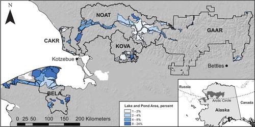
Figure 2. Mean annual air temperature for Kotzebue, Alaska, 1980–2018. National Weather Service data from NOAA Regional Climate Centers (2018). Points for years mentioned in the text are labeled. Means were computed for water years (October–September).

Annual precipitation fluctuated without a long-term trend during the study time interval at both Kotzebue and Bettles (Figure 3; Mann-Kendall trend tests for 2000–2017 for precipitation were nonsignificant at Kotzebue, p = .970, and Bettles, p = .596). Both stations experienced a decline in precipitation during the 2000 decade, followed by an increase starting in 2009 (Kotzebue) or 2011 (Bettles). Estimated potential evapotranspiration varied little between years (Figure 3). The net precipitation (precipitation minus potential evapotranspiration) at both stations ranged from near zero in dry years to more than 200 mm in wet years (Figure 3).

Figure 3. Annual precipitation and estimated annual potential evapotranspiration at Kotzebue (top) and Bettles (below). Precipitation and temperature data were obtained from NOAA Regional Climate Centers (2018). Evapotranspiration was estimated by the Hargreaves-Samani method, which is the most accurate at high latitudes of the simple temperature-based methods (Hargreaves and Allen 2003; Almorox, Quej, and Pau 2015).

Most of ARCN lies within the continuous permafrost zone (permafrost is present across 90 percent or more of the landscape; Jorgenson et al. 2008). Permafrost is discontinuous (present on 50–90 percent of the landscape) in the southern half of KOVA and the two southern lowland extensions of GAAR (Figure 1). The status of permafrost under water bodies in ARCN is mostly unknown. We can infer with certainty that permafrost is absent beneath large lakes in the discontinuous permafrost zone (e.g., Walker Lake in GAAR) and is present beneath small tundra ponds in continuous permafrost (Ling and Zhang 2003), but the state of permafrost in intermediate situations between these extremes is unknown.

Lakes of multiple origins and hydrologic conditions are present in ARCN, and ecological subsections provide a useful way to stratify the landscape into regions with relatively consistent hydrological and physiographic conditions (Larsen et al. 2017). Ecological subsections are areas of land with a relatively uniform climate and a consistent pattern of landforms, soils, and vegetation (Cleland et al. 1997). Subsection maps are available for all of ARCN (Jorgenson 2001; Jorgenson, Swanson, and Macander 2001; Boggs and Michaelson 2001; Swanson 2001a, 2001b). In addition, subsections provide a way to avoid various non-target areas, including (1) saltwater bodies (lagoons); (2) large floodplains (e.g., the Noatak River), where most of the water is in rivers and is subject to large year-to-year variations associated with the timing of the images; and (3) mountainous areas, where there are very few lakes but extensive terrain shadows are difficult to differentiate from water on Landsat images. Thus, I analyzed the lake-area trends for all lowland subsections in ARCN with at least 1 percent cover by surface-water bodies, excluding those where surface water was dominantly rivers or saltwater.

Subsections mapped in GAAR were less useful for summarizing lake trends, because they combine lake-rich valleys with neighboring uplands that have terrain-shadow problems and no lakes. Thus, in GAAR I created analysis regions that covered the lake-rich parts of each major river valley: Alatna, Itkillik, Killik, Kobuk, Koyukuk, Nigu, and Noatak. Although the analysis regions were named after major rivers, they were drawn to avoid actual river floodplains for the same reasons that river-dominated subsections were excluded (see earlier). Note that the GAAR analysis areas did not include the park’s large, deep mountain-valley lakes (Narvak, Nutuvukti, Selby, and Walker). These lakes have steep and stable shorelines, which gives them very constant surface areas, and they also have terrain-shadow problems that would make water mapping difficult.

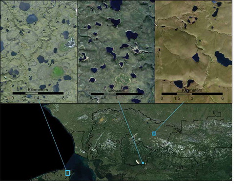
The geomorphological settings of the lakes in ARCN can be joined into three broad classes, based on the subsection reports cited previously and Hopkins (1963): (1) thaw-lake plains, (2) ice-rich loess over other unconsolidated deposits (glacial drift, volcanic ash and pumice, colluvial deposits), and (3) glacial drift and eolian sands with moderate to low ice content (Figure 4). The thaw-lake plains have ice-rich permafrost. Numerous shallow lakes overlap the outlines of older, drained lakes. Inter-lake surfaces are quite flat and only a few meters above the current lake levels. The ice-rich loess and loess over other deposits have lakes in depressions of thermokarst origin or mixed thermokarst and other (glacial, eolian) origin, separated by gently sloping uplands. Local relief ranges from a few meters to as much as 35 m on very ice-rich “yedoma” deposits (Shur et al. 2009). While drained lake basins are present in these areas, they do not blanket the surface as in thaw-lake plains. Ground ice contents in the thaw-lake plains and ice-rich loess correspond to the “high” ice-content class (more than 40 percent ice by volume in the upper 5 m) mapped by Jorgenson et al. (2008). The glacial drift and eolian sands are late Pleistocene deposits where lake basins appear to be primary depressions that have been only slightly modified by thermokarst. The glacial drift and eolian sands fall in the “low” (less than 10 percent ice by volume in the upper 5 m) and moderate (10–40 percent ice by volume in the upper 5 m) ice-content classes of Jorgenson et al. (2008).

Figure 4. Examples of generalized lake landscapes: ice-rich thaw lake plain (left), ice-rich deep silt (center), and glacial deposits with low to moderate ice content (right). The former two landscapes have lakes of mainly thermokarst origin and outlines of drained former lakes are visible on the images.

Methods

Imagery

I analyzed 30 m resolution Landsat data (Landsats 4–8) for the study area from the U.S. Geological Survey’s “Landsat Analysis-Ready Data” collection (ARD; Sauer and Dwyer 2018). The Landsat ARD contains atmospherically corrected surface reflectance data organized into a regular grid of 150 km × 150 km tiles. I analyzed all tiles in the study area with less than 40 percent cloud and less than 40 percent cloud shadow and from June to September of available years (1984–2018). The original scenes from which the Landsat ARD tiles were assembled consist of 185 km-wide swaths trending diagonally from northeast to southwest across the study area. Thus, multiple passes from different dates are required to obtain full coverage of the study area. Sporadic coverage was available for both the 1980s and 1990s, with between ten and thirty satellite passes over some part of the study area in June–September of just five total years in the two decades, and between zero and five passes in the other fifteen years. From 1999 to 2018 there were at least thirty satellite passes per year over some part of the study area.

Identification of surface water

I identified water by thresholding the surface reflectance of the Landsat shortwave infrared (SWIR) spectral band (band 5, 1.55–1.75 µm, for Landsats 4–7, and band 6, 1.566–1.651 µm, for Landsat 8). This simple method for identifying surface water from Landsat data was shown to be more accurate than computationally more complex methods based on multiple bands (Frazier and Page 2000; Roach, Griffith, and Verbyla 2012).

I chose the threshold SWIR reflectance value by comparing the reflectance of randomly located points inside lakes and ponds in the study area and on land. I generated random points at a density of one point per square kilometer of lake or pond water, using the National Hydrography Dataset (U.S. Geological Survey 2016) as the constraining feature, within the study-area subsections (Figure 1) of two Landsat ARD Alaska tiles (tiles h02v04, most of the lake region of BELA, and h04v03, most of KOVA and the southeastern part of NOAT). These points were additionally screened to ensure that they represented water by overlaying the IFSAR Orthorectified Radar Image Alaska (U.S. Geological Survey 2015) and selecting points where the radar image value was less than 51. SWIR values for all pixels not flagged as cloud or snow from all Landsat images on the two tiles were extracted to the random points. This amounted to approximately 42,000 SWIR values on tile h02v04 and 22,000 SWIR values on tile h04v03 (the latter had about half as much water area, hence the lower number of points). Histograms of the “water” point reflectances (Figure 5) show that most had Landsat SWIR reflectance values of less than 300 (i.e., reflectance of less than 3 percent). The long right tails on the “water” distributions consist mainly of mixed pixels containing land and water, or very shallow water. Very high values consist of land (i.e., water bodies in the training data that were not filled with water in all sample years) and clouds that the cloud mask missed.

Figure 5. Histograms of Landsat SWIR reflectance (times 10³) of random points in water bodies and on land in Landsat ARD tiles h02v04 and h04v03 for years 1984–2017.

An equal number of random points were generated inside the same subsections but on land (i.e., not in water bodies as defined by the NHD and the IFSAR image). Most of these “land” pixels had SWIR reflectance values of more than 1,500 (15 percent reflectance; Figure 5).

The SWIR threshold value of 600 (6 percent reflectance) was selected as a reasonable point within the transitional water-land pixels. A threshold of 600 results in 84–90 percent of the “water” training points being classified as “water” on the two test tiles, and 1 percent of the “land” training points to be classified as “water” in both test tiles. Thus, the estimated errors of omission of water are 16 percent and 10 percent of all water pixels for the two test tiles. These are overestimates of the true error rates, because these test data were drawn from all years, and some training pixels classified as water did in fact convert from water to land during the timespan of the Landsat record. The estimated error of commission rate (1 percent of land mapped as water) is also an overestimate, because some of the land pixels did indeed become water during the time span of the Landsat record. Note that because the surface is predominantly land, the map-wide error rates of omission and commission are actually quite similar: in a landscape that is about 6 percent water (a typical value for the study area) with 16 percent of the water pixels erroneously mapped as land, 0.06 × 0.16 = 0.0096, or 1 percent, of the map overall would be errors of omission (of water); likewise, if land covers 94 percent of the landscape with 1 percent erroneously mapped as water, 0.01 × 0.94 = 0.0094, or 1 percent, of the map overall would also be errors of commission (land erroneously mapped as water).

I used the quality band included with each Landsat ARD tile to mask out all pixels classified as “medium- to high-confidence” cloud and cloud shadow, snow, and ice. Cloud-free coverage was not available for the entire study area during June–September of every year, because of both the poor weather and the scan-line corrector failure that affected Landsat 7 starting in 2003. Thus, I aggregated data from three consecutive years and assigned the result to the middle year of the three. I stacked all “good” data from the three years and classified as “water” any pixel where more than half of the SWIR values for the three-year period were less than 600. Computations were made using the “raster” package in R (Hijmans 2015; R Core Team 2017).

Trend analysis

Consistent annual data became available starting in 1999, and thus my three-year running computations are from 2000 (1999–2001) to 2017 (2016–2018). I examined trends in the total area of water by subsection on the 2000–2017 time series using linear regression, segmented regression, and Mann-Kendall trend tests with Theil-Sen slope (Marchetto 2015; Muggeo 2017; R Core Team 2017). Segmented regression allows two or more different but connected linear trend lines to be fitted to a time series. Sporadic data from 1984–1989 were aggregated to produce a “1980s” water raster (plotted at year 1986 in the graphs) and similarly all data from the 1990s were aggregated to produce a “1990s” water raster (plotted at 1995 in the graphs).

Parts of BELA were missing 1980s imagery. The missing area amounted to 44 percent of the Bering Straits Lower Coastal Plain subsection and 25 percent of the Bering Straits Upper Coastal Plain subsection. I estimated values for the 1980s by assuming that the changes relative to the 1990s were the same in the no-data area of these two subsections as they were in the areas with data.

Results

Trends in lake area differed greatly between ecological subsections. Many subsections showed a strong minimum around 2010 and no clear long-term trend (Figure 6a). The 2010 minimum and subsequent increase match the multiyear fluctuations in precipitation (Figure 3). Some subsections showed a strong downward trend since 2000, with only a minor 2008–2010 minimum (Figure 6b). A few subsections showed an increasing trend in water area since 2000, usually with a jump in area after 2010 (Figure 6c).

Figure 6. (a) Water surface area versus year for the Noatak Glaciated Lowlands subsection (NOAT). This subsection showed a strong minimum at approximately 2010, with no significant long-term change. (b) Water surface area versus year for the Bering Straits Lower Coastal Plain subsection (BELA). This subsection showed a significant long-term decline, with a minor minimum at approximately 2008–2010. The estimated 2018 value was determined by subtracting from the 2017 value the area of lakes that drained abruptly in 2018. (c) Water surface area versus year for the Nigu River Valley (GAAR). This subsection showed an increase in water surface area from 2000 to 2017. Note the different scales of the three figures: the range of variation in (b) is large, more than 1 percent, compared to 0.3 percent and 0.25 percent in (a) and (b).

The strength of the long-term trend versus the precipitation-driven 2010 minimum was quantified by comparing the fit of a simple linear regression for 2000–2017 to a segmented regression of 2000–2017 with break points at both 2010 and 2013 (Table 1). Subsections with strong negative trends (the top seven rows in Table 1) and strong positive trends (the bottom six rows in Table 1) had relatively high ratios of r² (linear) to r² (segmented), indicating a fairly straight linear trend where segmenting adds little explanatory power. The middle group of seventeen subsections in Table 1 had weak overall trends and low ratios of r² (linear) to r² (segmented), indicating a good fit to a three-part segmented regression that follows fluctuations in precipitation.

Table 1. Lake area change 2000–2017 by ecological subsection^a.

Subsection	NPS Unit	Permafrost	Subsection Area (km^2)	Lake Area (%)	Slope (ha yr)^a	p Value	Ratio of r^2 (linear/segmented)	Past Ten Years vs. 1980–1990
Subsections with Decreasing Water Area 2000–2017
BSLCP	BELA	Thaw-lake plain	1,630	9.0	−71.6	<0.01	0.93	-
BSUCP	BELA	Ice-rich	1,327	6.2	−19.4	<0.01	0.73
NIP	KOVA	Ice-rich	750	1.3	−7.3	<0.01	0.71	-
IL	BELA	Ice-rich	339	23.5	−7.3	<0.01	0.59
AKP	KOVA	Ice-rich	381	1.5	−5.3	<0.01	0.72
WUL	CAKR	Ice-rich	351	0.9	−2.6	<0.01	0.52	-
LNM	CAKR	Ice-rich	97	4.2	−0.7	0.01	0.44
Subsections with Fluctuating Water Area 2000–2017
DU	BELA	Ice-rich	826	9.8	−2.9	0.54	0.07	+
NGL	NOAT	Ice-poor	655	4.6	−2.9	0.40	0.00
GBLCP	BELA	Thaw-lake plain	116	5.8	−1.3	0.20	0.07	+
ACP	CAKR	Thaw-lake plain	112	2.8	0.1	0.76	0.02	+
IMP	CAKR	Thaw-lake plain	18	9.1	0.2	0.52	0.26	+
KOY	GAAR	Ice-rich	230	2.5	0.3	0.79	0.00
AGU	NOAT	Ice-poor	231	11.8	0.7	0.40	0.08
KOB	GAAR	Ice-rich	240	1.3	0.7	0.10	0.18
MNU	NOAT	Ice-poor	544	4.6	0.8	0.50	0.04
NOA	GAAR	Ice-poor	177	6.8	0.9	0.32	0.43
AHW	KOVA	Ice-poor	142	12.1	2.4	0.26	0.19
GBUCP	BELA	Ice-rich	1,320	3.1	2.6	0.40	0.05	+
IGU	NOAT	Ice-poor	984	3.1	3.4	0.40	0.35
LNL	NOAT	Thaw-lake plain	404	10.5	6.4	0.60	0.31
UNB	NOAT	Ice-poor	2,475	2.0	8.1	0.21	0.30
NGU	GAAR	Ice-poor	207	3.9	1.5	0.09	0.60
KGU	NOAT	Ice-poor	584	3.0	2.6	0.07	0.43
Subsections with Increasing Surface Water 2000–2017
KZL	BELA	Ice-rich	226	4.7	1.7	0.04	0.38	+
ITK	GAAR	Ice-poor	31	17.5	0.4	0.02	0.57
KOP	CAKR	Thaw-lake plain	118	2.4	1.1	0.02	0.62	+
KIL	GAAR	Ice-poor	92	5.7	2.8	0.01	0.84
NIG	GAAR	Ice-poor	78	4.7	1.1	<0.01	0.96
ALA	GAAR	Ice-poor	23	22.3	1.6	<0.01	0.98

^aNPS Unit; see Figure 1.

Slope. Rate of change in water surface area, ha yr^a. Theil-Sen non-parametric slope.

p value. Probability value for the Mann-Kendall trend test.

Ratio of r²: linear/segmented. Ratio of r² of linear regression to r² of a three-part segmented regression with break points at the years 2010 and 2013.

Past ten years vs. 1980–1990. A dash (-) indicates that water area in all of the past ten years (2008–2017) was less than both the 1980s and 1990s values. A plus (+) indicates that water area was greater in all of the past ten years than in the 1980s or 1990s.

Subsections with significant declines in water area since 2000 (the top seven subsections in Table 1) contained 43 percent of the water surface in the study area. Subsections with significant water loss all have ice-rich substrates and lakes of dominantly thermokarst origin (Table 1, top group; Figure 7, red zones). Subsections where the variance in water area is dominated by the 2010 minimum (driven by precipitation) and the overall trend is insignificant (Table 1, middle group) account for most of the remaining water area (52%) in the study area. These lakes have both ice-rich and ice-poor settings (Figure 7, light blue and pink zones). The subsections with positive trends in lake area since 2000 (Table 1, bottom group) represent a relatively minor amount of water area (4 percent of the total water area). They are in two contrasting locations: mountain valleys in GAAR on ice-poor substrates, and two small ice-rich lowland areas in BELA and CAKR (Figure 7, dark blue zones).

Figure 7. (a) Lake-area change in the western part of the study area (BELA), (b) the central part (CAKR, KOVA, and NOAT), and (c) the eastern part (GAAR). Subsection colors give the overall trend in water area 2000–2017: red for decreasing and blue for increasing, with bright colors indicating significance at p < .05. Circles mark the location of lakes that drained, with circle size proportional to the area lost and shading keyed to the decade of drainage: white (1985–2000), gray (2001–2010), and black (2011–2017). Drained lakes are defined as those that had half or less as much surface area in 2017 as 2000. The year they first lost 25 percent or more of their area was identified as the year of drainage.

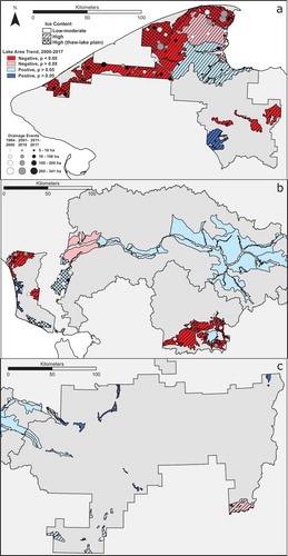
The rate of water-area loss in the Bering Straits Lower Coastal Plain (BSLCP) in BELA was by far the fastest of any subsection, more than 70 ha yr⁻¹ since 2000 (Table 1). The BSLCP is the northernmost, coastal, cross-hatched zone in BELA in Figure 7a. The adjacent Bering Straits Upper Coastal Plain also had a high rate of lake loss of nearly 20 ha yr⁻¹. The subsections with water-area gains (Table 1, bottom) had much more modest rates, less than 3 ha yr⁻¹.

The water area in several of the subsections with downward trends since 2000 has, for all of the past ten years, been lower than it was in either the 1980s or 1990s; these are labeled as - in the far-right column of Table 1. More subsections have for all of the past ten years been above the 1980s and 1990s levels; these are labeled as + in Table 1. The subsections with higher recent values than in the 1980s and 1990s all had nonsignificant or positive trends since 2000.

Numerous lakes in the study area lost the majority of their area during the course of one to several years and did not recover. I identified these “drained” lakes as those that lost at least 50 percent of their area during the study time interval and were at least 5 ha in area to begin with. There were 108 “drained” lakes, and they were concentrated in the lowland subsections with declining total lake area (Figure 7). The total water area that was lost in 2000–2017 from the “drained” lakes in the seven subsections with significant downward trends (Table 1) amounted to 19.5 km², an amount that actually exceeded the total loss of water area (from all lakes) in these subsections during that time interval (14.6 km²). In other words, without lake drainage the water area in these subsections would have increased, and the drained lakes more than account for the loss of water area in these subsections.

The amount of water-area loss resulting from lake drainage and the number of new drained lakes varied by year (Figure 8). Approximately 40 percent of the lake-area loss from 2000 to 2017 in the “drained” lakes occurred in 2005–2007. Most of the lake area lost in 2005–2007 (7.3 km² out of 8.6 km² total in 2005–2007) was from the Bering Straits Lower Coastal Plain subsection in BELA, mentioned earlier.

Figure 8. (a) Loss of water area by year of the 108 lakes that were identified as “drained” during 2000–2017. These were lakes that had half or less as much surface area in 2017 as 2000, and had a maximum surface area of 5 ha or more. (b) Count of new lake-drainage events by year, 2000–2017. The final values (2018) on both plots were estimated from partial coverage of the study area in September 2018.

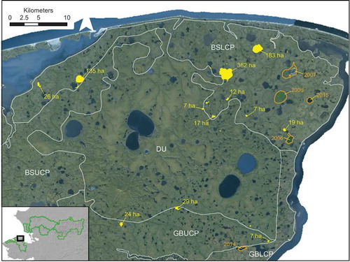
Preliminary data indicate that a lake-drainage event occurred in 2018 that was larger than the one in 2005–2007. NPS staff reported multiple lakes in northern BELA that suddenly drained laterally through outlet channels in 2018. Because my computations of lake areas are derived from a composite of three years of data, the 2018 drainage events had a negligible effect on my last data point (for 2016–2018, plotted at 2017). However, cloud-free Landsat scenes from September 2018 were available for portions of the study area, including northern BELA. By applying the same thresholding value (600) to the SWIR band of these scenes, I obtained a preliminary 2018 water map of northern BELA and far southwestern NOAT. Sixteen lakes with areas greater than 5 ha in 2017 had lost more than 50 percent of their area by September 2018. The total area lost from these sixteen lakes between 2017 and 2018 was 9.1 km², which is already greater than the ARCN-wide total for the 2005–2007 drainage event (8.6 km²). The Bering Straits Lower Coastal Plain lost the bulk of this area (7.6 km², Figure 9), and this lost area was used to estimate a 2018 value for the subsection (Figure 6b). The estimated 2018 value for the BSLCP is well below the value that would be expected from extrapolating the 2000–2017 trend line.

Figure 9. Lake loss in northeastern BELA. Areas that lost water between 2017 and 2018 are shaded in yellow, and those more than 5 ha in area are labeled in yellow with area lost, in hectares. Pre-2017 lake losses are outlined and labeled with the year in orange. The white lines outline ecological subsections (Jorgenson 2001) used as analysis areas: BSLCP, Bering Straits Lower Coastal Plain; BSUCP, Bering Straits Upper Coastal Plain; DU, Devil Uplands; GBLCP, Goodhope Bay Lower Coastal Plain; GBUCP, Goodhope Bay Upper Coastal Plain. The background image is from 2010 (Alaska Geospatial Council 2011).

Discussion

Much of the study area experienced declining water area during 2000–2017, despite the fact that net precipitation did not decline during this time. Water surface area declined in lake-rich lowlands with ice-rich permafrost where water bodies are predominantly of thermokarst origin. Most of the sudden lake-drainage events that occurred during the study time interval were in these zones of declining overall water area, and the drainage events are sufficient to explain the lake loss.

In contrast, in areas with permafrost of low to moderate ice content and lake basins of non-thermokarst (mostly glacial) origin, sudden lake drainage events were rare, the water surface area fluctuated in response to year-to-year variations of net precipitation, and long-term trends were weak. Much of this area had more water area in the past ten years (2008–2017) than in the 1980s or 1990s. Lake outlets are not highly susceptible to thermoerosion in these relatively ice-poor, mostly morainal landscapes. This study confirms Larsen et al.’s (2017) conclusion that the geomorphic setting of arctic lakes is a strong determinant of their properties.

Sudden lake drainage events in northern BELA usually occur because of thermoerosion of outlets (Jones et al. 2011). High water levels resulting from high precipitation can cause over-topping of lake banks, followed by thermoerosion of a new outlet and lake drainage (Jones and Arp 2015). Thaw subsidence in ice-wedge networks also can create new or lower water-flow pathways across the land surrounding lakes. Degradation of ice wedges associated with a warming climate has been widely observed in northern Alaska (Jorgenson, Shur, and Pullman 2006; Liljedahl et al. 2016). The last major episode of lake drainages in ARCN (2005–2007) occurred during a time of generally declining net precipitation, and it followed an episode of record high temperatures in 2003–2004: the record mean annual air temperature at Kotzebue of −3.6°C that had stood since 1978 was broken in 2003 and 2004 (−3.0°C in both years). This warm weather could have caused some local thaw of ground ice that facilitated the thermoerosion of new drainage outlets during the 2005–2007 lake-drainage episode.

The lake-drainage episode that began in the summer of 2018 has already exceeded the totals from the 2005–2007 episode. Conditions since 2014 have been the warmest on record: the 2003 record mean annual air temperature at Kotzebue (−3.0°C) was broken in 2014 (−2.0°C), again in 2016 (−1.6°C), and again 2018 (−0.9°C), with 2015 and 2017 also above normal (−2.8°C and −3.5°C). In addition, the winter of 2017–2018 was the second snowiest on record at Kotzebue (NOAA Regional Climate Centers 2018). Thus, both high water levels and warm temperatures apparently made conditions favorable for the thermoerosion of new lake-drainage outlets in 2018.

The rate of surface-water loss in the Bering Straits Lower Coastal Plain (BSLCP) subsection in northern BELA is particularly alarming: here a water area of approximately 9.5 percent of the surface in the 1980s and 1990s had declined to less than 8.5 percent by 2018. During the period 2000–2017 the rate of water loss averaged about 700 ha per decade, with about 14,500 ha of water remaining in 2017. The loss of an additional 760 ha by sudden drainage in 2018 suggests a significant acceleration in the rate of water loss. This area is rich in water-dependent wildlife, including yellow-billed loons (G. adamsii) and Pacific loons (Gavia pacifica), which nest on lakeshores and forage in lakes. These two species occur in low density, yet appear to have fully occupied the available lake habitat in BELA and CAKR (Schmidt, Flamme, and Walker 2014). Hence, any loss of lake area is likely to directly impact their populations. Loss of lowland lakes by drainage and their transition to lowland meadow and shrub habitats is one of the important ecotype transitions that is expected to affect arctic tundra environments as a result of climate warming (Jorgenson et al. 2015).

Why the different responses of lakes in different subsections with ice-rich permafrost? The BSLCP is probably uniquely vulnerable because it was rich in lakes to begin with, and the very low-relief inter-lake areas are blanketed with ice-wedge polygons. Thus minimal subsidence or thermoerosion along readily available ice-wedge networks was sufficient to trigger lake drainage. In contrast to the water loss in the BSLCP, two small ice-rich subsections experienced significant water-area increase during 2000–2017 (in far southern BELA, Figure 7a, and along the west coast of CAKR, Figure 7b). These areas showed increases in water area along lake margins, without any major drainage events. Gradual growth of lakes and ponds in ice-rich terrain by thermokarst along the shoreline is typical (e.g., Jones et al. 2011). Lake-drainage events are infrequent, and the lack of any drainage events in these small areas during a limited time period could be the result of a small sample, and thus should not be interpreted as evidence that these lakes will be stable throughout the long term. The Lower Noatak Lowlands subsection of far southwestern NOAT is another ice-rich, thaw-lake plain that experienced little change in 2000–2017, but had four large lake drainages in the 1980s and one in 2007 that was mostly outside the park boundary. Complete drainage of a 63 ha lake there in 2018 shows that this area is still vulnerable to lake loss. The Devil Uplands (DU, Figure 9) is ice rich but contains four large, stable maar lakes of non-thermokarst origin (Begét, Hopkins, and Charron 1996) that mask the trends in smaller, thermokarst lakes. Here and in neighboring ice-rich subsections with weak trends, thermokarst lakes are more deeply inset in basins tens of meters deep that appear to be somewhat more stable than the shallow basins of thaw-lake plains.

Lake loss resulting from infiltration of water after the loss of permafrost below lakes was observed by Yoshikawa and Hinzman (2003) in the discontinuous permafrost zone of the southern Seward Peninsula and is possible in the study area, especially in the Kobuk River valley (in KOVA and southwestern GAAR) where permafrost is discontinuous and presumably thinner. Warming of shallow lakes so that ice no longer freezes to the bottom has already allowed permafrost loss to begin under many shallow arctic lakes, even while permafrost remained generally stable on surrounding lands (Arp et al. 2016). Warming is expected to increase the prevalence of lakes with through-taliks where deep infiltration could occur (Burn 2005).

Modeling of permafrost temperatures and active layers by Panda, Marchenko, and Romanovsky (2016) suggests that in the ice-rich lowlands of BELA, CAKR, southern KOVA, and far western NOAT permafrost temperatures were −2°C to −4°C in 2000–2009, and in most areas will rise to −2°C to −1°C by the 2050s and  —1 to +1°C by the 2090s. These predictions were based on the moderate A1B emission scenario of the IPCC Fourth Assessment Report (IPCC 2007). Given that ground ice is responsible for much of the relief between lakes and surrounding land in these lowlands, and that ice wedges are common here, and on melting form a natural network of drainage channels, we can expect lake drainage and loss by thermoerosion of outlets to continue in these areas as warming continues. Where the climate is cold enough to maintain permafrost, restabilization of degraded ice wedges is possible (Kanevskiy et al. 2017). However, if mean annual ground temperatures rise above 0°C in these lake-rich zones, as is possible by the end of this century, eventual complete degradation of ice wedges is inevitable, with associated widespread formation of new lake-drainage outlets.

Conclusions

The area occupied by lakes and ponds of thermokarst origin in the National Parks of northern Alaska declined significantly since the start of Landsat records in the 1980s. This decline was the result of the sudden drainage of lakes by the thermoerosion of lateral outlets. Episodes with more frequent lake drainages occurred in 2005–2007 and in 2018, in both cases following two or more years with record warm temperatures. In contrast, the area of lakes and ponds in depressions of other (non-thermokarst) origin fluctuated in response to short-term variations in net precipitation, without strong long-term trends. The relatively long time series and complete coverage available from the Landsat record indicates that thermokarst lake losses represent a long-term, effectively irreversible trend that is associated with a warming climate. Lake drainage is of special concern because it represents a direct loss of habitat for aquatic wildlife.

Acknowledgments

All imagery was provided at no cost by the U.S. Geological Survey. Thanks to Melanie Flamme, Jared Hughey, Ben Jones, Amy Larsen, and Sarah Swanson for field observations and photos of drained lakes, and for helpful discussions. Thanks to Celia Miller, Jon O’Donnell, Eric Wald, and an anonymous reviewer for helpful comments on the manuscript.

Disclosure statement

No potential conflict of interest was reported by the author.

Additional information

Funding

This study was funded by the Inventory and Monitoring Division of the National Park Service, U.S. Department of the Interior.

References

- Alaska Geospatial Council. 2011. SDMI SPOT 5 2.5-meter statewide imagery. Anchorage, Alaska. http://gis.dnr.alaska.gov/terrapixel/cubeserv/ortho?DATASTORE=SPOT5_SDMI_ORTHO_CIR&SERVICE=WCS&REQUEST=GetDescription.
- Almorox, J., V. H. Quej, and M. Pau. 2015. Global performance ranking of temperature-based approaches for evapotranspiration estimation considering Köppen climate classes. Journal of Hydrology 528:514–22. doi:10.1016/j.jhydrol.2015.06.057.
- Arp, C. D., B. M. Jones, G. Grosse, A. C. Bondurant, V. E. Romanovsky, K. M. Hinkel, and A. D. Parsekian. 2016. Threshold sensitivity of shallow Arctic lakes and sublake permafrost to changing winter climate. Geophysical Research Letters 43 (12):6358–65. doi:10.1002/2016GL068506.
- Begét, J. E., D. M. Hopkins, and S. D. Charron. 1996. The largest known maars on earth, Seward Peninsula, Northwest Alaska. Arctic 62–69. http://www.jstor.org/stable/40511986.
- Boggs, K., and J. Michaelson. 2001. Ecological subsections of Gates of the Arctic National Park and Preserve. Anchorage: Inventory and Monitoring Program, National Park Service, Alaska Region. https://irma.nps.gov/App/Reference/DownloadDigitalFile?code=151098&file=GAAR_EcologicalSubs_final.pdf.
- Burn, C. R. 2005. Lake‐bottom thermal regimes, western Arctic coast, Canada. Permafrost and Periglacial Processes 16 (4):355–67. doi:10.1002/ppp.542.
- Cleland, D. T., P. E. Avers, W. Henry McNab, M. E. Jensen, R. G. Bailey, T. King, and W. E. Russell. 1997. National hierarchical framework of ecological units. In Ecosystem management applications for sustainable forest and wildlife resources, ed. M. S. Boyce and A. Haney, 181–200. New Haven, CT: Yale University.
- Earnst, S. L., R. A. Stehn, R. M. Platte, W. W. Larned, and E. J. Mallek. 2005. Population size and trend of yellow-billed loons in Northern Alaska. The Condor 107 (2):289–304. doi:10.1650/7717.
- Frazier, P. S., and K. J. Page. 2000. Water body detection and delineation with Landsat TM data. Photogrammetric Engineering and Remote Sensing 66 (12):1461–68.
- Grosse, G., B. Jones, and C. Arp. 2013. Thermokarst lakes, drainage, and drained basins. Treatise on Geomorphology 8:325–53. https://www.sciencedirect.com/science/article/pii/B9780123747396002165?via%3Dihub.
- Hargreaves, G. H., and R. G. Allen. 2003. History and evaluation of Hargreaves evapotranspiration equation. Journal of Irrigation and Drainage Engineering 129 (1):53–63. doi:10.1061/(ASCE)0733-9437(2003)129:1(53).
- Hijmans, R. J. 2015. Raster: geographic data analysis and modeling (version R package version 2.3-40). Vienna, Austria: R Foundation for Statistical Computing. http://CRAN.R-project.org/package=raster.
- Hopkins, D. M. 1949. Thaw lakes and thaw sinks in the Imuruk Lake area, Seward Peninsula, Alaska. Journal of Geology 57:119–31. http://www.jstor.org/stable/30063635.
- Hopkins, D. M. 1963. Geology of the Imuruk Lake area, Seward Peninsula, Alaska. Geological Survey Bulletin 1141–C, US Government Printing Office, Washington, DC. http://pubs.usgs.gov/bul/0974c/report.pdf.
- Hussey, K. M., and R. W. Michelson. 1966. Tundra relief features near Point Barrow, Alaska. Arctic 19 (2):162–84.
- IPCC. 2007. Climate change 2007: Synthesis report. contribution of working groups I, II and III to the fourth assessment report of the Intergovernmental Panel on Climate Change. Geneva, Switzerland: IPCC. https://www.ipcc.ch/report/ar4/syr/.
- Jones, B. M., and C. D. Arp. 2015. Observing a catastrophic thermokarst lake drainage in northern Alaska. Permafrost and Periglacial Processes 26 (2):119–28. doi:10.1002/ppp.1842.
- Jones, B. M., C. D. Arp, M. S. Whitman, D. Nigro, I. Nitze, J. Beaver, A. Gädeke, C. Zuck, A. Liljedahl, and R. Daanen. 2017. A lake-centric geospatial database to guide research and inform management decisions in an Arctic watershed in Northern Alaska experiencing climate and land-use changes. Ambio 46 (7):769–86. doi:10.1007/s13280-017-0915-9.
- Jones, B. M., G. Grosse, C. D. Arp, M. C. Jones, K. M. Walter Anthony, and V. E. Romanovsky. 2011. Modern thermokarst lake dynamics in the continuous permafrost zone, northern Seward Peninsula, Alaska. Journal of Geophysical Research: Biogeosciences (2005–2012) 116 (G2):G00M03. doi:10.1029/2011JG001666.
- Jorgenson, M. T., D. K. Swanson, and M. Macander. 2001. Landscape-level mapping of ecological units for the Noatak National Preserve, Alaska. Anchorage: Inventory and Monitoring Program, National Park Service, Alaska Region. https://irma.nps.gov/App/Reference/DownloadDigitalFile?code=419154&file=NOAT_EcologicalSubsections.pdf
- Jorgenson, M. T. 2001. Ecological subsections of Bering Land Bridge National Preserve. Anchorage: Inventory and Monitoring Program, National Park Service, Alaska Region. https://irma.nps.gov/App/Reference/DownloadDigitalFile?code=418816&file=BELA_EcologicalSubsections.pdf.
- Jorgenson, M. T., B. G. Marcot, D. K. Swanson, J. C. Jorgenson, and A. R. DeGange. 2015. Projected changes in diverse ecosystems from climate warming and biophysical drivers in northwest Alaska. Climatic Change 130 (2):131–44. doi:10.1007/s10584-014-1302-1.
- Jorgenson, M. T., J. E. Roth, P. F. Miller, M. J. Macander, M. S. Duffy, A. F. Wells, G. V. Frost, and E. R. Pullman. 2009. An ecological land survey and landcover map of the Arctic Network. Natural Resource Technical Report ARCN/NRTR-2009/270, National Park Service, Fort Collins, CO. https://irma.nps.gov/App/Reference/Profile/663934.
- Jorgenson, M. T., K. Yoshikawa, M. Kanevskiy, Y. Shur, V. Romanovsky, S. Marchenko, G. Grosse, J. Brown, and B. Jones. 2008. Permafrost characteristics of Alaska. Fairbanks: Institute of Northern Engineering, University of Alaska Fairbanks. http://www.cryosphericconnection.org/resources/alaska_permafrost_map_dec2008.pdf.
- Jorgenson, M. T., and Y. Shur. 2007. Evolution of lakes and basins in northern Alaska and discussion of the thaw lake cycle. Journal of Geophysical Research: Earth Surface 112:F2. doi:10.1029/2006JF000531.
- Jorgenson, M. T., Y. L. Shur, and E. R. Pullman. 2006. Abrupt increase in permafrost degradation in arctic alaska. Geophysical Research Letters 33:2. doi: 10.1029/2005GL024960.
- Kanevskiy, M., Y. Shur, T. Jorgenson, D. R. N. Brown, N. Moskalenko, J. Brown, D. A. Walker, M. K. Raynolds, and M. Buchhorn. 2017. Degradation and stabilization of ice wedges: Implications for assessing risk of thermokarst in northern Alaska. Geomorphology 297:20–42. doi:10.1016/j.geomorph.2017.09.001.
- Larsen, A. S., J. A. O’Donnell, J. H. Schmidt, H. J. Kristenson, and D. K. Swanson. 2017. Physical and chemical characteristics of lakes across heterogeneous landscapes in Arctic and subarctic Alaska. Journal of Geophysical Research: Biogeosciences. doi:10.1002/2016JG003729/full.
- Lawler, J. P., S. D. Miller, D. Sanzone, J. Ver Hoef, and S. B. Young. 2009. Arctic Network vital signs monitoring plan. Natural Resource Report NPS/ARCN/NRR-2009/088, National Park Service, Fort Collins, Colorado. https://irma.nps.gov/DataStore/Reference/Profile/661340.
- Liljedahl, A. K., J. Boike, R. P. Daanen, A. N. Fedorov, G. V. Frost, G. Grosse, L. D. Hinzman, Y. Iijma, J. C. Jorgenson, N. Matveyeva, et al. 2016. Pan-Arctic ice-wedge degradation in warming permafrost and its influence on tundra hydrology. Nature Geoscience 9:312–18. doi:10.1038/NGEO2674.
- Ling, F., and T. Zhang. 2003. Numerical simulation of permafrost thermal regime and talik development under shallow thaw lakes on the Alaskan Arctic Coastal Plain. Journal of Geophysical Research: Atmospheres 108:D16. doi:10.1029/2002JD003014.
- Livingstone, D. A., K. Bryan, and R. G. Leahy. 1958. Effects of an Arctic environment on the origin and development of freshwater lakes. Limnology and Oceanography 3 (2):192–214. doi:10.4319/lo.1958.3.2.0192.
- Mackay, J. R. 1988. Catastrophic lake drainage, Tuktoyaktuk Peninsula area, District of Mackenzie. Paper 88-1D, Geological Survey of Canada, Ottawa. doi:10.4095/122663.
- Marchetto, A. 2015. Rkt: Mann-Kendall test, seasonal and regional Kendall tests. R package version 1.4. Vienna, Austria: R Foundation for Statistical Computing. http://CRAN.R-project.org/package=rkt.
- Muggeo, V. M. R. 2017. Package ‘Segmented.’ Biometrika 58 (525–534):516.
- Nitze, I., G. Grosse, B.M. Jones, C.D. Arp, M. Ulrich, A. Fedorov, and A. Veremeeva. 2017. Landsat-based trend analysis of lake dynamics across northern permafrost regions. Remote Sensing 9 (7):640. doi:10.3390/rs9070640.
- NOAA Regional Climate Centers. 2018. XmACIS Version 1.0.38. XmACIS Version 1.0.38. 2018. http://xmacis.rcc-acis.org/.
- Panda, S. K., S. S. Marchenko, and V. E. Romanovsky. 2016. High-resolution permafrost modeling in the Arctic Network of National Parks, Preserves and Monuments. Natural Resource Report NPS/ARCN/NRR-2016/1366, National Park Service, Fort Collins, Colorado. https://irma.nps.gov/DataStore/Reference/Profile/2237720.
- PRISM Climate Group. 2009. Mean monthly temperature for Alaska 1971–2000. Annual mean average temperature for Alaska 1971-2000. Corvallis, OR: Oregon State University. http://prism.oregonstate.edu.
- R Core Team. 2017. R: A language and environment for statistical computing (version 3.4.1). Vienna, Austria: R Foundation for Statistical Computing. http://www.R-project.org.
- Riordan, B., D. Verbyla, and A. David McGuire. 2006. Shrinking ponds in subarctic Alaska based on 1950–2002 remotely sensed images. Journal of Geophysical Research: Biogeosciences (2005–2012) 111 (G4). doi: 10.1029/2005JG000150.
- Roach, J., B. Griffith, D. Verbyla, and J. Jones. 2011. Mechanisms influencing changes in lake area in Alaskan boreal forest. Global Change Biology 17 (8):2567–83. doi:10.1111/j.1365-2486.2011.02446.x/full.
- Roach, J. K., B. Griffith, and D. Verbyla. 2012. Comparison of three methods for long-term monitoring of boreal lake area using Landsat TM and ETM+ imagery. Canadian Journal of Remote Sensing 38 (4):427–40. doi:10.5589/m12-035.
- Roach, J. K., B. Griffith, and D. Verbyla. 2013. Landscape influences on climate-related lake shrinkage at high latitudes. Global Change Biology 19 (7):2276–84. doi:10.1111/gcb.12196.
- Sauer, B., and J. Dwyer. 2018. U.S. Landsat Analysis Ready Data (ARD) Data Format Control Book (DFCB). LSDA-1873 Version 4.0, US Geological Survey Earth Resources Observation and Science (EROS) Center, Sioux Falls, South Dakota. https://landsat.usgs.gov/sites/default/files/documents/LSDS-1873_US_Landsat_ARD_DFCB.pdf.
- Schmidt, J. H., M. J. Flamme, and J. Walker. 2014. Habitat use and population status of yellow-billed and Pacific loons in Western Alaska, USA. The Condor 116 (3):483–92. doi:10.1650/CONDOR-14-28.1.
- Sellmann, P. V., J. Brown, R. I. Lewellen, H. McKim, and C. Merry. 1975. The classification and geomorphic implications of thaw lakes on the Arctic Coastal Plain, Alaska. CRREL-RR-344, Cold Regions Research and Engineering Lab, Hanover, New Hampshire. http://www.dtic.mil/docs/citations/ADA021226.
- Shur, Y., M. Z. Kanevskiy, M. T. Jorgenson, D. Fortier, M. Dillon, E. Stephani, and M. Bray. 2009. Yedoma and thermokarst in the northern part of Seward Peninsula, Alaska. AGU Fall Meeting Abstracts C41:0443. http://adsabs.harvard.edu/abs/2009AGUFM.C41A0443S.
- Swanson, D. K. 2001a. Ecological units of Cape Krusenstern National Monument, Alaska. Anchorage: Inventory and Monitoring Program, National Park Service, Alaska Region. https://irma.nps.gov/App/Reference/Profile/584438.
- Swanson, D. K. 2001b. Ecological units of Kobuk Valley National Park, Alaska. Anchorage: Inventory and Monitoring Program, National Park Service, Alaska Region. https://irma.nps.gov/App/Reference/Profile/584437.
- Swanson, D. K. 2013. Surface water area change in the Arctic Network of National Parks, Alaska, 1985–2011: Analysis of Landsat data. Natural Resource Data Series NPS/ARCN/NRDS—2013/445, Fort Collins, Colorado. https://irma.nps.gov/App/Reference/Profile/2193078.
- Swanson, D. K. 2017. Landscape patterns and dynamics monitoring protocol for the Arctic Network: Narrative. Natural Resource Report NPS/ARCN/NRR-2017/1380, National Park Service, Fort Collins, Colorado. https://irma.nps.gov/DataStore/Reference/Profile/2238342.
- U.S. Geological Survey. 2015. IFSAR Orthorectified Radar Image (ORI) Alaska. U.S. Department of the Interior, Geological Survey. https://lta.cr.usgs.gov/ifsar_ori.
- U.S. Geological Survey. 2016. NHD user guide. U.S. Department of the Interior, Geological Survey. https://nhd.usgs.gov/userguide.html.
- Yoshikawa, K., and L. D. Hinzman. 2003. Shrinking thermokarst ponds and groundwater dynamics in discontinuous permafrost near Council, Alaska. Permafrost and Periglacial Processes 14 (2):151–60. doi:10.1002/ppp.451/full.