Potential shifts in zooplankton community structure in response to changing ice regimes and hydrologic connectivity

ABSTRACT

Changing Arctic climate may alter freshwater ecosystems as a result of warmer surface waters, longer open-water periods, reduced wintertime lake ice growth, and altered hydrologic connectivity. This study aims to characterize zooplankton community composition and size structure in the context of hydrologic connectivity and ice regimes in Arctic lakes. Between 2011 and 2016, we sampled the phytoplankton, zooplankton, and fish communities from a set of representative lakes on the Arctic Coastal Plain (ACP) of northern Alaska to determine potential food web responses to changing Arctic ecosystems. Multivariate analyses showed that time from ice-out had a strong influence on zooplankton community structure and that seasonal succession of zooplankton differed between lakes with varying hydrologic connectivity. Trends were observed suggesting that large-bodied zooplankton (Daphnia, calanoid copepods) may be more prevalent in poorly connected lakes with low fish diversity. Large-bodied zooplankton displayed higher biomass in lakes with high occurrences of bedfast ice, while small-bodied zooplankton (Bosmina, rotifers) displayed highest biomass in deeper lakes with low occurrences of bedfast ice. Our results contribute to limited knowledge of zooplankton in remote lakes of the ACP and suggest that the anticipated changes to aquatic ecosystems in the Arctic may include energetically less efficient plankton food webs.

KEYWORDS:

• Arctic lakes
• bedfast ice
• climate change
• Daphnia
• fish predation

Introduction

More than 25 percent of lakes on Earth are located in the northern high latitude region (Lehner and Döll 2004) and can occupy 20–40 percent of the landscape in Arctic lowland regions (Grosse, Jones, and Arp 2013; Muster et al. 2017). Better understanding of the controls on food web dynamics in these ubiquitous aquatic ecosystems is of importance to local communities who rely on fish and water birds for subsistence, and globally in relation to migratory birds and fishes that rely on these habitats for summer foraging and breeding (Sibley et al. 2008; Schmidt, Flamme, and Walker 2014; Arp et al. 2019). These important ecosystems are responding rapidly to Arctic climate change. Surface area of Arctic lakes has both increased and decreased in response to changes in hydroclimate and permafrost stability across the Arctic (Smith et al. 2005; Jones et al. 2009, 2011; Labrecque et al. 2009; Arp et al. 2011, 2015; Lantz and Turner 2015). Increased air temperatures and increased winter precipitation over the past several decades have resulted in warmer lake surface (O’Reilly et al. 2015) and bed (Arp et al. 2016) temperatures, as well as decreased lake ice cover duration (Smejkalova, Edwards, and Dash 2016) and ice thickness (Arp, Jones, and Grosse 2013; Surdu et al. 2014; Arp et al. 2016). Following these changes, hydrologic connectivity responses between lakes and streams have been variable and complex (Lesack and Marsh 2007, 2010) and are highly uncertain given projections of hydrologic intensification in the Arctic (Wrona et al. 2006; Rawlins et al. 2010). The observed and predicted changes occurring in Arctic lakes may impact primary production (and subsequently higher trophic levels) via regulation of temperature, light availability, and mixing regimes (Vincent et al. 2013), while changes in hydrologic connectivity can impact food web structure via increased or decreased fish mobility and colonization potential (Laske et al. 2016).

Zooplankton are key intermediaries in aquatic food webs, transferring energy from primary producers to fish and higher consumers. Large-bodied zooplankton can suppress phytoplankton populations through grazing (Carpenter and Kitchell 1996), while fish predation has long been known to be the primary determinant for species composition and size structure of freshwater zooplankton communities (Hrbacek 1962; Brooks and Dodson 1965). Large-bodied crustaceans, particularly daphnids, are more preferable to fish planktivores from an energetic efficiency viewpoint and are selectively grazed through size-discriminant predation (Brooks and Dodson 1965). Where fish predation is intense, zooplankton communities are often dominated by small crustaceans and rotifers (Jeppesen et al. 2017). Lakes at lower latitudes with fish populations maintained year round display mostly small-bodied crustacean zooplankton since grazing pressure is strong (Brucet et al. 2013; Havens et al. 2015). When no fish are present, energy flow in plankton food webs of freshwater lakes (i.e., the degree of top-down control of phytoplankton growth by herbivorous zooplankton) is strongly influenced by the species composition and size structure of crustacean zooplankton communities (Persson et al. 2007). The size of planktonic cladocerans increases with increasing latitude and decreasing temperature (Gillooly and Dodson 2000), while metabolic processes, feeding rates, and reproductive activities decrease (Hart and Bychek 2011). Arctic lakes are known to have generally low aquatic invertebrate diversity (Rautio et al. 2008), and are often characterized by having few or no fish (Hershey et al. 2006; Power, Reist, and Dempson 2008; Laske et al. 2016). Accordingly, the importance of top-down control on zooplankton populations by planktivores in Arctic lakes is well-recognized (O’Brien, Buchanan, and Haney 1979; Schmidt and O’Brien 1982; Luecke and O’Brien 1983). Large cladocerans may persist in temperate lakes with high macrophyte coverage that provide sufficient refuge from planktivores (Jeppesen et al. 1998); however, Arctic lakes are typically too nutrient-poor to maintain large macrophyte communities, and thus Arctic zooplankton are highly vulnerable to predation by planktivorous fish.

Research on Arctic lakes suggests that connectivity and ice regimes predict fish community structure and abundance (Lesack and Marsh 2010; Laske et al. 2016), such that these physical attributes should also indirectly regulate zooplankton communities and size structure. Deeper lakes retain liquid water below floating ice and can provide winter refugia for some fish species given favorable environmental conditions. Thus, for lakes in which ice is frozen to the lake bed by the end of winter (bedfast ice lakes) fish colonization during the summer is required to exert grazing pressure on crustacean zooplankton populations, which is dependent on the degree of connectivity to deeper lakes or river systems where overwinter habitat is available (Haynes et al. 2014). Bedfast ice lakes also become ice-free consistently earlier than deeper, floating ice lakes (Arp et al. 2015), allowing for an earlier start to an otherwise short growing season for both phytoplankton and zooplankton and an extended period during which predation pressure is low. Recent trends suggest longer open-water periods among all types of high latitude lakes (Duguay et al. 2006; Smejkalova, Edwards, and Dash 2016) with expected longer growing seasons for phytoplankton and zooplankton communities.

Aquatic habitat connectivity is recognized as a primary mechanism allowing fish colonization during the growing season in Arctic lakes (Hershey et al. 1999, 2006). One projected consequence of changing arctic climate and associated hydrologic intensification is an increase in connectivity between Arctic lakes (Arp et al. 2019), which would likely result in an increase in fish species richness (Laske et al. 2016). Haynes et al. (2014) determined that fish distribution in the lakes of the Arctic Coastal Plain (ACP) was controlled by lake size, potential for colonization, and suitable depth for overwintering. Most streams in the drainage network of the ACP originate in lakes and about one third of the lakes are thought to have continuous stream connectivity during the open-water season (Arp et al. 2012b). The remaining lakes may be connected ephemerally to varying degrees during snowmelt and periods of higher summer rainfall (Jones et al. 2017). Ephemeral connectivity is essential for fish to colonize productive lakes with high bedfast ice lacking overwintering source populations. Even in deeper lakes that support overwintering habitat, but without stable or sustained connections, certain fish species are typically absent or at very low abundance (Laske et al. 2016) and the results on zooplankton communities should be apparent.

We hypothesized that the degree of hydrologic connectivity (a proxy for the ability of fish to colonize) and ice regimes (overwintering habitat and growing season length) in Arctic lake systems would be reflected in the taxonomic composition and size structure of the zooplankton communities. We predicted that lakes that were well-connected to the drainage network in spring would display small-bodied crustacean communities and lakes that were isolated from surface water connections and/or that froze solid to the bed would be most likely to have large-bodied crustacean zooplankton communities. We also predicted that zooplankton community composition would change along the course of a season, with larger forms dominant early in the season and smaller forms dominant later in the season, when fish colonization would be more likely to have occurred. Accordingly, we selected a range of lakes based on connectivity and ice regime attributes to quantify zooplankton composition and size structure seasonally and yearly in a representative ACP watershed, Fish Creek, to address these hypotheses. Observed warming air and permafrost temperatures and increased precipitation since 1999 (Arp et al. 2012b; Urban and Clow 2014), shifting lake ice regimes since 1980 (Arp et al. 2012a), and permafrost degradation since 1982 (Jorgenson, Shur, and Pullman 2006) in this watershed suggest a range of climate and environmental changes that will impact its freshwater ecosystems. Our biological results are placed in the context of these observed and anticipated future changes to lake-rich Arctic landscapes to refine predictions of freshwater food web dynamics.

Materials and methods

Study sites

The Fish Creek Watershed (FCW) drains a 4,900 km² area in northern Alaska, USA, approximately midway between Utqiaģvik (formerly Barrow) and Prudhoe Bay, entirely within the National Petroleum Reserve in Alaska (NPR-A) (Figure 1). Continuous permafrost occurs throughout this region reaching depths to 400 m except under numerous thermokarst lakes and river courses (Jorgenson, Shur, and Osterkamp 2008). Lakes are dominant landforms and ecosystems in the FCW with over 4,000 lakes (> 1 ha) covering 19% of the land surface (Jones et al. 2017). Many lakes in the eolian sand deposits have deep (up to 20 m) central basins within troughs of a stabilized dune field referred to as the Pleistocene or Ikpikpuk Sand Sea (Carter 1981). Shallower lakes in the lower portion of the watershed are primarily of thermokarst origin (Jorgenson and Shur 2007). Smaller, yet abundant, riverine lakes occur along the major alluvial rivers created by meander cut-offs as oxbow lakes and are also subject to thermokarst expansion.

Figure 1. (a) Sample locations and timing in the (b) Fish Creek Watershed in northern Alaska, USA, approximately midway between Utqiaģvik and Prudhoe Bay along the Beaufort Sea coast and entirely within the National Petroleum Reserve – Alaska (NPR-A).

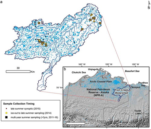
The lake-centric geospatial database described in Jones et al. (2017) was used to guide the selection of forty lakes for this study, which represent a range of connectivity to streams and rivers (isolated to flow through). A range of lake depths were also sampled, some shallow enough to freeze solid in the winter, and others deep enough to provide refugia for overwintering fish communities. Lake morphometric characteristics are provided in Table S1. All study lakes except for two (CC3 and CC4) were sampled in early August 2015 for synoptic characterization at the peak of growing season. A subset of sixteen lakes were also sampled in 2014 four times from mid-June to mid-August to capture within open-water season variability in plankton composition, abundance, and size. Additionally, six of these lakes had also been previously sampled in mid-July 2011 in association with baseline environmental monitoring related to petroleum development and fourteen of these lakes (including the 2011 set) were also sampled in mid-July 2012 and 2013. In total, this represented a plankton dataset of 142 individual samples collected over a six-year period with corresponding environmental data. Though a relatively short period, the year 2014 had a very late ice-out and cool summer, while 2015 had an exceptionally early ice-out and warm summer (Arp et al. 2015). The winters of 2011, 2012, and 2014 were very warm with thinner ice growth, and 2013 was cold with thicker ice; this variation in winter and summer climatology helps provide a wider range of lake limnological conditions and plankton responses captured in this study.

Plankton sampling and environmental characterization

The majority of sampling was conducted from a floatplane which allowed us to visit multiple lakes in this vast roadless region within a period of several days. For smaller water bodies, an inflatable raft was used to access central portions of lakes and ponds. Zooplankton were collected using a 30.5 cm mouth diameter tow net (WildCo™, 80 μm mesh size) using both vertical and horizontal tows depending on lake depth and emergent macrophyte densities. Vertical tows were performed when lake depth was approximately 1.5 m or greater, so that the cod end did not disturb the lake bed. Depending on lake size and observed surficial heterogeneity, three vertical tows of >0.75 m depth from the surface were typically made per lake at uniformly distributed locations and these samples were then composited. When lake depth was less than 1.5 m, horizonal tows were performed. Horizontal tow volumes were quantified using the zooplankton net diameter and the distance of water covered by the tow net, determined by the tape on the tow line. Zooplankton samples were rinsed from net mesh and collection cups and stored in 50 percent ethanol solution. Due to the limitations imposed by net mesh size, some rotifers and nauplii (organisms <80 µm in length) may have been missed by the tows. Phytoplankton were collected concurrently at the same distributed locations by surface grab samples, composited, and stored in Lugol’s solution prior to analysis.

At the same time and locations as plankton sampling, we measured surface water temperature with a water quality sonde (YSI 6600-v2). Twenty lakes were instrumented with temperature sensors at the bed (Onset U20-001, ±0.2°C) and surface (Onset U12-015, ±0.1°C), which were moored from buoys at lake-center locations year-round as part of the CALON, FCWO, and Fish CAFÉ projects, and logged at hourly intervals. These sensor systems were used to measure timing of ice-out as described in Arp, Jones, and Grosse (2013) and synoptic aerial surveys carried out by Fish CAFÉ Project (Arp et al. 2019) in 2013–2015 were used to evaluate melt-out status. Standardized Water Temperature (SWT) was calculated as the average surface water temperature over the seven-day period prior to each sample collection. The SWT metric was used in our analyses rather than point measurements from the water quality sonde to eliminate interlake variability related to visit timing within the day or among days and to provide a more accurate biophysical representation of thermal conditions experienced by plankton prior to sampling. Average ice-out (from instrumented lakes) was June 19, with earliest ice-out occurring on May 15 and latest ice-out occurring on July 1. During the study period, 2014 had the latest ice-out date and 2015 had the earliest ice-out date. However, within a given year inter-lake variation is controlled primarily by ice regime (i.e., bedfast ice or floating ice conditions) (Arp et al. 2015). Average ice-on timing during the study period was October 1 and ranged from September 17 to October 14. For lakes where no water temperature buoys were installed, SWT was estimated from the multiple regression equation of point water temperature measurements, lake depth, and time from ice-out (r² = 0.79, p < 0.001). In addition to sensor indicated ice-out timing, aerial surveys were conducted in mid-June of both 2014 and 2015 to record ice-cover conditions of study lakes in the FCW. The metric “time from ice-out” represents the open-water period between the day in which lake ice cover was reduced to less than 10 percent and the day that the lake was sampled. In several cases during the mid-June sampling period of 2014, lakes were still partly ice covered such that time from ice-out had a negative value (i.e., lake sampled before ice-out occurred).

Lake morphometric and hydrologic indices follow the lake-centric geospatial database reported in Jones et al. (2017). Briefly, lake connectivity to stream networks is based on a Connectivity Index from 1 to 4, where 1 is isolated (no inflow or outflow), 2 is temporary headwater (ephemeral outflow only), 3 is perennial headwater (continuous outflow during open-water season), and 4 is flowthrough (both inflowing and outflowing stream connections during the open-water season). For geospatial classification in Jones et al. (2017), these classes were calculated based on field measured discharge according to dominant terrain units and their corresponding contributing area thresholds from a digital elevation model (DEM) using ArcGIS hydrology toolsets. These stream-lake connectivity classes were also evaluated independently based on field observations and the overall accuracy of the index was determined to be 72 percent. The metric “bedfast ice index,” which represents lake morphometry relative to maximum ice thickness, was determined from synthetic aperture radar (SAR) satellite imagery acquired in late winter 2009 to classify lake ice as bedfast (frozen to the bed, typically depths <1.6 m) or floating (liquid water below ice, typically depths >1.6 m) (Grunblatt and Atwood 2014). The surficial percentage of floating ice (not grounded to bed) was also quantified for each lake based on the same data, such that for a lake with 100 percent floating ice, the entire bed is deeper than ~1.6 m. Lakes with entirely bedfast ice (i.e., 0 percent floating ice) are shallow throughout. The total accuracy of the lake ice classification scheme was 89 percent (Grunblatt and Atwood 2014).

Fish sampling

Fish were sampled during 2014 and 2015 at 22 lakes using a multi-gear approach based on Haynes et al. (2013), which developed a method and species-specific detection probabilities from sampling eighty-six lakes on the ACP. Gear types included gill nets and minnow traps deployed in shallow and deep water, nearshore fyke nets, and beach seines. Two variable-mesh multifilament gill nets measuring 38 m × 1.8 m with five panels ranging in bar mesh size from 1.3 to 6.5 cm were used. One gill net (pelagic gill net) was deployed perpendicular to the shoreline at the surface within the littoral zone, with the bottom of the net just above the lake floor. The second gill net (benthic gill net) was weighted so that it floated submerged with the lead line on the lake bottom. We deployed the benthic gill net at the deepest zone of the lake (as determined by depth sounder transects), perpendicular or oblique to the shoreline. Gill nets were checked every 2–3 h and removed on the third check. Eight Gee-style galvanized steel minnow traps (2.5 cm opening with 6 mm mesh) were baited with preserved salmon eggs. Four of these traps were deployed individually in shallow water along the shoreline (shore minnow traps) and four traps were sunk with weights in the deepest zone of the lake (deep minnow traps). After 12 h, traps were checked for fish, baited again, and replaced. Traps were checked for fish and removed after 24 h. Two fyke nets were deployed to sample the shoreline, each having a hoop net constructed of 0.3 cm stretched mesh and had a frame opening of 1.1m × 1.1 m, followed by five sequential hoop frames spaced 0.8 m apart and measuring 0.6 m × 0.6 m in size. Attached to the hoop net were two 15.2 m × 1.2 m wings and a 30.5 m × 1.2 m centerline with 0.6 cm stretched mesh. Wings and centerline had float lines and weighted lead lines. The hoop net had three net throats within the frame measuring 15 cm × 23 cm at the middle of each throat. Nets were set either in the morning or the evening at separate locations within a lake. Nets were checked twice for fish, once after approximately 12 h and again after 24 h when the nets were pulled. If a lake had a stream connection, one fyke net was set adjacent the connection, but did not entirely block it. Centerlines were set perpendicular from the shore except in lakes with very shallow shelf zones (<0.4 m depth) that exceeded the length of the centerline. At locations with extensive shallow shelves, the centerline was set away from shore (but still perpendicular) such that the fyke net was closer to the drop off and would sample the deeper water. Dip nets (3 mm mesh; two opening sizes 28 cm × 38 cm × 20 cm and 41 cm × 41 cm × 41 cm) were used on the lakeshore. Nets were swept along the lake bottom adjacent to shore for three 8 min intervals. Set times for each gear type were calculated in order to have high expected Cumulative Detection Probabilities (CDP) for several fish species (Alaska blackfish (Dallia pectoralis) CDP = 0.99; Arctic grayling (Thymallus arcticus) CDP = 0.80, broad whitefish (Coregonus nasus) CDP = 0.97; least cisco (Coregonus sardinella) CDP = 1.00; ninespine stickleback (Pungitius pungitius) CDP = 1.00; slimy sculpin (Cottus cognatus) CDP = 0.71), although data did not exist to calculate probabilities for all species encountered. Fish species identifications were made in the field immediately following collection.

Zooplankton analysis

Water samples collected for zooplankton analyses were preserved with a 50 percent ethanol solution, packaged, and shipped to BSA Environmental Services, Inc., in Beachwood, OH. Prior to microscopic analysis, sample volume was measured and each sample was homogenized using a magnetic spinner at low speed. A subsample was taken using a wide-bore volumetric pipette and transferred into an Utermöhl chamber. Appropriate aliquots were examined at 100X magnification on Wilovert inverted microscopes, and a minimum tally of 400 organisms per sample was reached (Lund, Kipling, and LeCren 1958). Zooplankton species identification (Table S2) was accompanied by up to 20 individual length and/or width measurements for each identified species. Biomass estimates were based on established length/width relationships (Dumont, van de Velde, and Dumont 1975; McCauley 1984; Lawrence et al. 1987). For cladocerans, the length was measured from the tip of the head to the end of the body (shell spines excluded). For copepods, the length was measured from the tip of the head to either the insertion or end of the caudal ramus, depending on species (McCauley 1984; Lawrence et al. 1987). Rotifers were typically measured from the tip of the head to the end of the body (spines, toes, etc., excluded), except for species in which lorica width was required to compute biomass (e.g., Conochilus spp. and Trichocerca spp.). Biomass was computed for the appropriate number of individuals for each sample location and the arithmetic mean biomass was multiplied by the species abundance to produce a species biomass for each sample (McCauley 1984). Zooplankton carbon content was assumed to be 50 percent of dry mass (Latja and Salonen 1978). Mean values for both zooplankton size and biomass were computed for each lake, then compared and tested for significant differences using single-factor ANOVA across connectivity index categories. To avoid pseudoreplication (Hurlbert 1984), means for biomass and length of individual zooplankton groups were calculated for each individual lake using all samples that were taken from that lake, including samples taken during different years and at different points within a year. These whole-lake means were computed prior to testing for significant differences in biomass and length between connectivity categories.

Phytoplankton analysis

Phytoplankton samples collected in 2014, 2015, and 2016 were preserved with 2 percent Lugol’s solution for subsequent laboratory analysis. Samples were homogenized, filtered through 0.45 µm membrane filters, and analyzed on Leica DMLB compound microscopes using the membrane filtration technique (McNabb 1960). Samples were analyzed at 630X magnification for random field and full strip counts, as well as 400X magnification for half-filter counts. Species were enumerated and identified to the lowest possible taxonomic level (Table S3) to a threshold of 400 natural units including colonies, filaments, and unicells. Biovolume estimates were determined using genus-specific geometric shapes most similar to the algal cell form (Hillebrand et al. 1999). Ten organisms per taxon (when possible) were measured for biovolume calculations. Phytoplankton carbon content was estimated as described in Rocha and Duncan (1985), and Z:P (zooplankton:phytoplankton) ratio was calculated using both zooplankton and phytoplankton carbon content. Mean values for phytoplankton biovolume were computed for each lake, then compared and tested for significant differences using single-factor analysis of variance (ANOVA) across connectivity index categories. Z:P was also calculated for each lake (using means if multiple samples were taken at an individual lake) and compared across connectivity index categories using single-factor ANOVA.

Canonical correlation analysis

Thirty-four zooplankton taxa identified from samples collected between 2011 and 2016 were used in the Canonical Correlation Analysis (CCA) using PRIMER 6 (Clarke and Gorley 2006). Only those samples with corresponding water quality data were used in analyses, resulting in 142 individual samples. The biomass data were standardized, and a Bray-Curtis resemblance matrix was created. A sample-matched, normalized matrix of five environmental variables consisting of SWT, time from ice out, lake area, lake depth, and bedfast ice index was analyzed against the zooplankton biomass resemblance matrix using the Canonical Analysis of Principal Coordinates (CAP) function of the PERMANOVA+ add-on in PRIMER 6. Following the CCA, samples were plotted on ordination diagrams using the first two CAP axes. Samples on the ordination diagram were coded by month of collection, and the biomass values of individual zooplankton taxa were superimposed over the CCA plot.

Cluster analysis: Fish species

A matrix of eleven fish species and twenty-two lakes was constructed using catch per unit effort data. Specimens identified in the field as “unspecified whitefish” were excluded from analysis. The data were standardized, and a Bray-Curtis resemblance matrix was created. A complete linkage dendrogram was produced using the Clustering Analysis function in PRIMER 6. Mean values for environmental and planktonic variables were compared and tested for significant differences using single-factor ANOVA across three clusters.

Results

Connectivity index

Comparisons between the four connectivity index categories using whole-lake means (n = 40 lakes) showed some variation amongst abiotic parameters (Table 1), although no significant differences were observed. SWT was lowest on average in connectivity 1 lakes (8.0°C) and highest in connectivity 4 lakes (10.7°C). Isolated lakes (connectivity index 1) tended to be smaller (mean surface area of 0.2 km²) and shallower (mean depth of 2.2 m) than less isolated lakes, with highest mean bedfast ice index (57.8). Time from ice out was shortest on average in connectivity index 1 lakes (approximately 32 days), but highest on average in connectivity index 2 lakes (approximately 50 days) indicating that this variable does not trend monotonically across connectivity indices.

Table 1. Mean (± standard error) standardized water temperature (SWT), time from ice out, lake area, lake depth, and bedfast ice by connectivity index categories (1 = isolated, 4 = high hydrological connectivity).

Connectivity Index Category	1	2	3	4
n	5	17	10	8
SWT (°C)	8.0 (± 0.5)	9.5 (± 0.1)	9.6 (± 0.2)	10.7 (± 0.8)
Time from Ice Out (days)	31.6 (± 5.9)	50.4 (± 3.4)	40.0 (± 4.4)	42.6 (± 4.7)
Lake Area (km^2)	0.2 (± 0.04)	2.3 (± 0.4)	3.1 (± 0.7)	1.2 (± 0.7)
Depth (m)	2.2 (± 0.3)	4.3 (± 0.9)	4.9 (± 1.5)	2.8 (± 0.8)
Bedfast Ice Index	57.8 (± 13.0)	54.7 (± 7.2)	55.5 (± 8.7)	45.9 (± 10.9)

Single-factor ANOVAs (F(3,36)) followed by post-hoc (Tukey’s Honestly Significant Difference (HSD)) comparisons were performed to test for significant differences between connectivity categories for each major zooplankton group. The only zooplankton group to show significant differences in biomass (p < 0.01) between connectivity index categories was Cyclopoida (Connectivity 1 differed significantly from all other connectivity categories, Mean = 6.10 µg d.w. L⁻¹, Standard Deviation = 5.39 µg d.w. L⁻¹) (Table 2). As with biomass, the only significant difference (p < 0.05) observed between connectivity index categories in terms of zooplankton body size was for Cyclopoida (single factor ANOVA (F(3,26)) (Table 3). Post-hoc comparisons using the Tukey’s HSD test indicated that the mean length for Cyclopoida in connectivity 1 lakes (Mean = 1.64 mm, Standard Deviation = 0.77 mm) differed significantly from mean Cyclopoida length in connectivity 3 lakes (Mean = 0.80 mm, Standard Deviation = 0.33 mm), but did not differ significantly for any other pairs of connectivity categories. The highest mean carbon ratio for C-zooplankton:C-phytoplankton (Table 4) was also observed in connectivity index 1 lakes; however, no significant differences in carbon ratios between connectivity categories were detected. These findings highlight the high degree of variability in zooplankton communities among lakes.

Table 2. Mean (± standard error) biomass (µg d.w. L⁻¹) of Daphnia spp. (n = 4 species), other cladocerans (n = 7 species), total cladocerans (n = 11 species), Heterocope sp., Diaptomidae (n = 6 species), other Calanoida (n = 3 species), total Calanoida (n = 10 species), total Cyclopoida (n = 5 species), total Rotifera (n = 54 species), and total phytoplankton biovolume (μm³ L⁻¹) for the connectivity index categories (1 = isolated, 4 = high hydrological connectivity); n represents the number of lakes in each connectivity index category.

Connectivity Index Category	1	2	3	4
n	5	17	10	8
Daphnid Biomass	41.5 (± 20.1)	33.5 (± 21.5)	9.5 (± 7.1)	18.3 (± 13.8)
Other Cladoceran Biomass	0.3 (± 0.1)	2.0 (± 1.2)	1.4 (± 0.7)	12.3 (± 8.5)
Total Cladoceran Biomass	41.8 (± 20.1)	35.6 (± 21.3)	11.0 (± 7.1)	30.5 (± 14.3)
Heterocope Biomass	1.44 (± 0.94)	0.94 (± 0.52)	0.42 (± 0.32)	0.15 (± 0.15)
Diaptomidae Biomass	12.61 (± 5.59)	19.03 (± 13.76)	2.56 (± 2.14)	1.68 (± 0.70)
Other Calanoida Biomass	0.04 (± 0.04)	0.01 (± 0.01)	0.52 (± 0.42)	0.14 (± 0.14)
Total Calanoida Biomass	14.1 (± 6.0)	19.98 (± 14.22)	3.5 (± 2.5)	2.0 (± 0.8)
Cyclopoida Biomass	**6.10 (± 2.41)	0.20 (± 0.11)	0.18 (± 0.09)	0.14 (± 0.13)
Rotifera Biomass	0.56 (± 0.27)	1.49 (± 0.33)	3.29 (± 1.05)	2.38 (± 0.72)
Phytoplankton Biovolume	1.34 x10^9 (± 4.81 × 10^8)	9.50 x 10^8 (± 1.19 × 10^8)	1.39 x 10^9 (± 1.74 × 10^8)	1.29 x 10^9 (± 1.85 × 10^8)

** denotes significant difference at p < 0.01.

Table 3. Mean (± standard error) weighted length (mm) for Daphnia spp. (n = 4 species), other cladocerans (n = 7 species), total cladocerans (n = 11 species), total Calanoida (n = 10 species), and total Cyclopoida (n = 5 species) for the connectivity index categories (1 = isolated, 4 = high hydrological connectivity); n represents the number of lakes in each connectivity index category. Mean weighted length based on relative abundance.

Connectivity Index Category	1	2	3	4
n	5	17	10	8
Daphnid Length	1.45 (± 0.25)	1.39 (± 0.27)	1.04 (± 0.25)	1.18 (± 0.34)
Other Cladoceran Length	0.37 (± 0.03)	0.34 (± 0.01)	0.43 (± 0.08)	0.42 (± 0.05)
Total Cladoceran Length	0.92 (± 0.20)	0.97 (± 0.23)	0.67 (± 0.16)	0.75 (± 0.15)
Calanoida Length	1.38 (± 0.19)	1.19 (± 0.12)	1.07 (± 0.14)	1.12 (± 0.15)
Cyclopoida Length	*1.64 (± 0.35)	0.87 (± 0.16)	0.80 (± 0.11)	0.99 (± 0.24)

* denotes significant difference at p < 0.05.

Table 4. Mean (± standard error) ratio of C-zooplankton to C-phytoplankton (Z:P) for the connectivity index category (1 = isolated, 4 = high hydrological connectivity).

	n	C-zooplankton:C-phytoplankton
Connectivity 1	5	0.19 (± 0.08)
Connectivity 2	17	0.10 (± 0.04)
Connectivity 3	10	0.03 (± 0.01)
Connectivity 4	6	0.07 (± 0.04)

Although no significant differences were observed between connectivity categories for all other zooplankton groups, some trends were apparent. Highest mean values for daphnid biomass (41.5 μg d.w. L⁻¹), total cladoceran biomass (41.8 μg d.w. L⁻¹) and total cyclopoid biomass (6.10 μg d.w. L⁻¹) were observed in isolated (connectivity 1) lakes (Table 2). The large, predatory calanoid copepod Heterocope septentrionalis also showed highest mean biomass in connectivity 1 lakes. Mean rotifer biomass was lowest on average (0.56 μg d.w. L⁻¹) in connectivity 1 lakes. Non-daphnid cladoceran biomass was lowest on average in connectivity 1 lakes (0.3 μg d.w. L⁻¹) and highest in connectivity 4 lakes (12.3 μg d.w. L⁻¹). Phytoplankton biovolume was lowest in connectivity 2 lakes (9.50 x 10⁸ μm³ L⁻¹) and highest in connectivity 3 lakes (1.39 x 10⁹ μm³ L⁻¹), showing no clear trend in terms of relative connectivity when using whole lake means. Analysis of weighted length by connectivity index also showed that larger-bodied zooplankton tended to be more prevalent in connectivity 1 lakes (Table 3). Mean weighted length was highest for daphnids (1.45 mm) in isolated lakes and decreased with increasing connectivity. Similarly, both Calanoida and Cyclopoida tended to be larger in isolated (connectivity 1) lakes (1.42 and 1.27 mm, respectively), generally decreasing in mean length with increasing connectivity. Other cladoceran length was seemingly unaffected by connectivity index, ranging from 0.34–0.43 mm. Interestingly, mean size for daphnids, Calanoida, and Cyclopoida was slightly elevated in connectivity 4 lakes compared to connectivity 3 lakes; however, since no significant differences were detected, this observation was likely due to factors other than connectivity regime.

Canonical correlation analysis (CCA)

CCA compared thirty-four zooplankton taxa and five environmental variables, producing two canonical axes with moderately strong correlations. Axes one and two explained 74 percent and 57 percent of the total variance observed, respectively. Standardized water temperature exhibited a moderate positive correlation with the first axis (CAP1, 0.396) and a moderate negative correlation with the second axis (CAP2, −0.340). Time from ice-out displayed a strong positive correlation with the first axis (0.903). Lake depth was moderately negatively correlated with the second axis (−0.479), while bedfast ice index displayed a strong positive correlation with the second axis (0.757). Lake area was weakly correlated with both axes.

The ordinational distribution of D. middendorffiana revealed an association with shallow lakes and high bedfast ice extents (Figure 2a). Ordination of D. longiremis biomass suggested peak biomass occurred later following ice-out at warmer temperatures in lakes with low bedfast ice extents, while D. pulex complex tended to be more dominant in shallower lakes with high bedfast ice extents (Figure 2b). Similar to D. middendorffiana, the Calanoida biomass ordination showed an association with smaller lakes with high bedfast ice extents (Figure 2c), although calanoids were frequently observed at lower biomass in many deeper lakes with warmer temperatures. The majority of observations of Calanoida also fell on the positive side of the first axis, suggesting peak biomass occurred later following ice-out. A strong positive correlation with standardized water temperature was observed for B. longirostris (Figure 2d), suggesting that this species is strongly controlled by water temperature, either directly or indirectly. Ordinational distribution of B. longirostris also suggested later occurrence of peak biomass following ice-out, in deeper lakes with low bedfast ice extents. Distribution of Cyclopoida on the ordination diagram differed from all other crustacean groups, with highest biomass observed in samples collected shortly after ice-out at low water temperatures (Figure 2e). Rotifers exhibited an association with warmer temperatures and deeper lakes with low bedfast ice extents (Figure 2e). The first CAP axis represents a gradient in terms of seasonality of sample collection, with those samples on the negative side of the first axis being primarily collected in June and those on the positive side of the first axis primarily collected in August (Figure 2f). In general, higher zooplankton biomass was found in later season samples for all groups, except for Cyclopoida, which showed highest biomass shortly following ice-out and rotifers, which were well distributed across the CAP1 axis.

Figure 2. Canonical Correlation Analysis (CCA) ordination diagrams for the zooplankton biomass CCA (n = 145) [(a) Daphnia middendorffiana; (b) Daphnia longiremis (light gray bubbles) and Daphnia pulex complex (dark gray bubbles); (c) Calanoida (d) Bosmina longirostris; (e) rotifers (light gray bubbles) and Cyclopoida (dark gray bubbles)]; and (f) samples coded by month. (a)–(e): each bubble represents biomass (zooplankton ordinations (a–e) µg d.w. L⁻¹) or biovolume (phytoplankton ordination (f) µm³ L⁻¹) for an individual sample, and bubble size corresponds to the magnitude of biomass in one sample according to the scale to the right of each ordination diagram. (f): each point represents a single sample, coded by month.

Complete linkage cluster analysis: Fish species

The complete linkage dendrogram revealed three clusters consisting of ten, eight, and four lakes, respectively (Figure 3), which were determined based on similarity in fish community composition. Ninespine stickleback was by far the most abundant fish species in all clusters (Table S4). Cluster 1 showed the lowest fish species richness, with only five species in total. Cluster 2 had the highest fish species richness, with eleven species. Cluster 3 had eight species. Aside from ninespine stickleback, the most abundant fish species in Cluster 1 was arctic grayling; however, this species only occurred in three of the ten lakes, and was not observed in any of the connectivity 1 lakes from this cluster. In clusters 2 and 3, the second most abundant fish species was least cisco. Three of the ten lakes in cluster 1 were classified as connectivity 1 lakes; only one other connectivity 1 lake was sampled for fish species and was included in cluster 3 (Figure 3). Despite variation in zooplankton communities and physical characteristics (Tables 5 and 6), no significant differences in either zooplankton biomass or physical characteristics between clusters were detected.

Table 5. Mean (± standard error) values for species richness, lake area, lake depth, and bedfast ice extent for each lake cluster identified from the complete linkage dendrogram.

	n	Mean Fish Species Observed	Lake Area (km^2)	Depth (m)	Bedfast Ice Extent
Cluster 1	10	2.2	1.5 (± 0.5)	3.1 (± 1.0)	53.6 (± 9.6)
Cluster 2	8	5.6	2.9 (± 0.8)	4.7 (± 1.2)	43.9 (± 5.0)
Cluster 3	4	4.8	2.7 (± 1.3)	6.1 (± 3.4)	50.6 (± 17.2)

Table 6. Mean (± standard error) biomass (µg d.w. L⁻¹) of B. longirostris, Calanoida, Cyclopoida, Daphnia spp., Rotifers, total zooplankton biomass and total phytoplankton biovolume (μm³ L⁻¹)for each lake cluster identified from the complete linkage dendrogram performed on fish community composition in lakes.

	n	B. longirostris	Calanoida	Cyclopoida	Daphnia spp.	Rotifers	Total Biomass	Total Biovolume
Cluster 1	10	1.1 (± 0.8)	5.5 (± 2.3)	2.3 (± 1.2)	36.4 (± 14.8)	2.0 (± 0.8)	54.5 (± 17.3)	1.0 x 10^9 (± 1.6 × 10^8)
Cluster 2	8	1.2 (± 0.5)	0.4 (± 0.3)	0.2 (± 0.1)	2.6 (± 1.8)	2.4 (± 0.6)	7.4 (± 2.9)	1.2 x 10^9 (± 2.3 × 10^8)
Cluster 3	4	1.5 (± 0.8)	4.8 (± 4.7)	3.1 (± 2.6)	13.7 (± 11.5)	3.0 (± 1.9)	34.1 (± 26.1)	1.1 x 10^9 (± 2.4 × 10^8)

Figure 3. Complete linkage dendrogram resulting from fish catch per unit effort (CPUE) data across 22 lakes. Clusters 1 through 3 represent ten, eight, and four lakes, respectively.

Seasonal trends

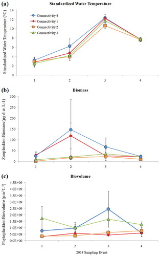
A subset of 64 zooplankton and phytoplankton samples from 16 different lakes collected in mid-June, late June, mid-July, and mid-August 2014 were analyzed according to connectivity index. The final sample for seasonal analysis (mid-August) was collected approximately 1.5 months prior to freezing, which consistently occurred in early October. Within our limited data set, some seasonal trends were observed. All four connectivity categories followed similar trends in temperature, beginning around 2–4°C in mid-June, increasing to 4–6°C by late June, increasing to 10–12°C by mid-July, the dropping to about 8°C by mid-August (Figure 4a). Flowthrough lakes (connectivity 4) warmed slightly more than other lakes between the first and second sampling events. Connectivity 1 lakes and connectivity 4 lakes displayed similar trends regarding the zooplankton community; mean biomass peaked in late June and continued to decline through July and August (Figure 4b). However, the increase in mean zooplankton biomass at the second sampling event was highly variable between lakes (n = 12) and was not statistically significant (single factor ANOVA, F(3,12) = 1.24, p = 0.34). Lakes in connectivity categories 2 and 3 did not show a great degree of change in total zooplankton biomass throughout the four sampling events. Phytoplankton biovolume was relatively consistent throughout the four sampling events for lakes with connectivity indices 1 and 2, despite seasonal fluctuations in temperature (Figure 4c). Both connectivity 3 and connectivity 4 lakes increased in total phytoplankton biovolume between sampling events 2 and 3 (late June to mid-July), then decreased by mid-August.

Figure 4. 2014 seasonal mean: (a) standardized water temperature, (b) zooplankton biomass, and (c) phytoplankton biovolume. Sampling events 1–4 correspond to mid-June, late June, mid-July, and mid-August, respectively. Data were analyzed according to connectivity index (connectivity 1, n = 16; connectivity 2, n = 16; connectivity 3, n = 20; connectivity 4, n = 12).

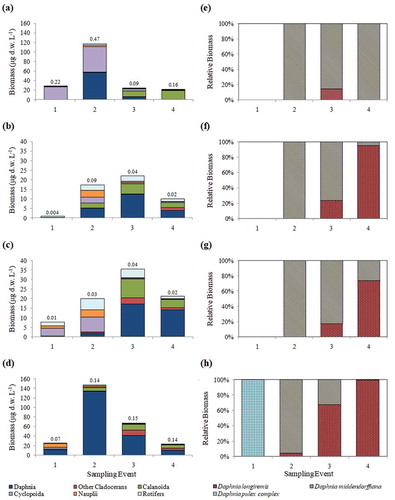
Zooplankton community composition also varied throughout the season between lakes with differing connectivity regimes (Figure 5). Isolated lakes were dominated by Cyclopoida in mid-June, then shifted to co-dominance of Cyclopoida and Daphnia (primarily D. middendorffiana) by the late-June. By mid-July, Calanoida made up approximately 50 perent of the total biomass, and by mid-August, Calanoida made up approximately 90 percent of the total biomass (Figure 5a). Lakes with connectivity indices of 2 and 3 were both dominated primarily by rotifers, nauplii, and Cyclopoida from early- to mid-June, then shifted to dominance by Daphnia spp. and Calanoida from mid-July to mid-August (Figure 5b–c). Connectivity 4 lakes were dominated primarily by Daphnia (D. pulex complex) and nauplii in mid-June, then shifted to over 90 percent dominance by Daphnia (primarily D. middendorffiana) by late-June (Figure 5d–h); however, this dominance was largely driven by a high abundance of D. middendorffiana in one lake. Daphnia spp. remained the dominant biomass producer in these lakes for the remainder of the season, but with larger numerical contributions from D. longiremis from mid-July to mid-August (Figure 5h); biomass of both Calanoida and non-daphnid cladocerans also made large contributions to total biomass later in the season. For both isolated and flowthrough lakes, rotifer biomass was low throughout the sampling season, while for lakes with intermediate flow regimes, rotifers made moderate contributions to total biomass throughout the summer. Z:P also varied seasonally and between lakes with varying degrees of connectivity (Figure 5a–d). The connectivity 1 lakes had overall highest Z:P ratios, which increased from 0.22 in mid-June to 0.47 by late June, then dropped to 0.09 by mid-July and increased again slightly to 0.16 by mid-August. Intermediate connectivity lakes had relatively low (<0.1) Z:P throughout the season. Connectivity 4 lakes had relatively low (0.07) Z:P in mid-June, then increased to 0.14–0.15 Z:P for the remainder of the summer.

Figure 5. Mean zooplankton biomass and mean relative biomass of Daphnia species for 2014 seasonal sampling. Sampling events 1–4 correspond to mid-June, late June, mid-July, and mid-August, respectively. Data are organized by connectivity index with (a) connectivity 1, total biomass, (b) connectivity 2, total biomass, (c) connectivity 3, total biomass, (d) connectivity 4, total biomass, (e) connectivity 1, relative daphnid biomass, (f) connectivity 2, relative daphnid biomass, (g) connectivity 3, relative daphnid biomass, and (h) connectivity 4, relative daphnid biomass. Connectivity 1, n = 4 lakes; connectivity 2, n = 4 lakes; connectivity 3, n = 5 lakes; connectivity 4, n = 3 lakes). Mean Z:P ratio is given above bars in (a)–(d).

Discussion

Factors controlling plankton communities

Historically, few studies have examined zooplankton populations in the ACP (Kling, Fry, and O’Brien 1992a; Kling et al. 1992b; Samchyshyna, Hansson, and Christoffersen 2008), primarily because of the remoteness of many potential sampling locations (Arp et al. 2019). In this study, sampling was limited by accessibility of remote lakes, both seasonally and interannually. The effort required to access some sites prevented concurrent sampling on a broad scale. As such, the data included in this study are both highly variable and highly valuable in terms of potential for ecological insight. Although it is possible that under-ice plankton populations were missed by our sampling regime (Hampton et al. 2017; Grosbois and Rautio 2018) or that peak biomass could have occurred later in the season, near autumn (Rautio, Sorvari, and Korhola 2000), the CCA showed that zooplankton communities within our study lakes were strongly influenced by seasonally variable parameters, with time from ice-out being the most important variable controlling species composition. Bedfast ice index was also strongly influential on zooplankton community composition, with larger bodied forms (Daphnia, calanoid copepods) exhibiting higher total biomass in lakes with higher bedfast ice extents and smaller bodied forms (Bosmina longirostris, rotifers) exhibiting higher total biomass in lakes with lower bedfast ice extents (i.e., higher fish colonization potential). This result supports our hypothesis that lakes which freeze solid to the bed would be dominated large-bodied crustacean zooplankton communities. Our hypothesis that zooplankton community composition would be comprised of larger forms early in the season and smaller forms later in the season however was only partially supported. Cyclopoid copepod biomass was highest early in the season, but other large forms including Daphnia spp. and calanoid copepods tended to dominate later in the season. High cyclopoid biomass observed in samples taken earlier in the season suggests quick maturity early on in the growing season, or possibly the occurrence of viable under-ice populations prior to ice-out. The most frequently observed cyclopoid copepod from this study, Cyclops scutifer, is known to exist in a dormant juvenile state in lake sediments at low temperatures, then to become reanimated after ice-out when water temperature warms (Elgmork 1962). In a recent study of under-ice zooplankton, all specimens of C. scutifer observed during winter were C-IV copepodites (Grosbois et al. 2017), which lends support to the idea that this species utilizes life-cycle adaptations to maximize survival. Cyclopoida was the only group of zooplankton that showed statistically significant differences in terms of biomass between lakes in different connectivity categories, displaying significantly higher biomass in isolated lakes compared to more connected systems. Since isolated lakes tended to be sampled earlier and at lower temperatures than more connected lakes (see Table 1), it is difficult to say whether the higher Cyclopoida biomass in those lakes was a result of hydrologic isolation or if it was a function of unintended bias due to earlier season sampling. Amongst lakes sampled concurrently in 2014, Cyclopoida were the dominant component of the zooplankton community in isolated lakes early in the season (through mid-June in a colder-than-average year). This finding suggests that both hydrology and seasonality may influence the ability of Cyclopoida to compete with other zooplankton groups.

While results indicated that ice regimes are closely tied to zooplankton community structure, it is difficult to draw firm conclusions as to whether zooplankton are influenced directly or indirectly by ice dynamics. Moderate correlations with both axes in the CCA suggest that zooplankton, like most Arctic taxa, are influenced by seasonal changes in temperature to some degree. Ice dynamics are intricately tied to distribution of Arctic fish species (Reist et al. 2006; Haynes et al. 2014). Although fish data were collected during this study, the data were insufficient to determine the extent to which ice dynamics may have impacted community composition. Thus, it is difficult to classify the relative influence of ice dynamics, fish, and hydrologic connectivity on zooplankton community and size structure. However, concurrent seasonal sampling from a limited number of sites in 2014 does highlight some fundamental differences in community succession patterns amongst lakes with differing hydrologic regimes. General patterns of succession—i.e., early dominance by Cyclopoida followed by dominance of Daphnia spp. and Calanoida—are in agreement with previous seasonal studies on Arctic lakes (Primicerio and Klemetson 1999). Lakes with differing connectivity regimes showed variation in Daphnia species composition, which may help to explain some of the variation in phytoplankton dynamics. In poorly connected lakes, the large species D. middendorffiana was the dominant daphnid species throughout the season, with limited contributions from other species. In lakes with moderate to high connectivity, D. middendorffiana was dominant through late June, but by mid-July and mid-August, the smaller, less efficient algal grazer D. longiremis was numerically more abundant. The dominance of D. middendorffiana in poorly connected lakes may be responsible for the suppression of phytoplankton growth from those lakes by mid-July, while dominance of D. longiremis (possibly due to selective predation on D. middendorffiana by planktivorous fish moving in later in the summer) may be partially responsible for the increase of phytoplankton in highly connected lakes at the mid-July sampling point. Higher Z:P ratios in poorly connected lakes at the late-June sampling point support this notion; however, since Z:P ratios are based on carbon-carbon values and not biomass:biovolume, it is possible that zooplankton in poorly connected lakes may be obtaining the majority of their carbon from benthic sources earlier in the season. Benthic algal mats have been shown to be an important food source for Daphnia in some Arctic lakes (Mariash et al. 2014), and considerable evidence indicates that a large portion of the carbon assimilated by Arctic zooplanktivorous fish originates from benthic sources (e.g., Hershey et al. 1999; Sierzan, McDonald, and Jensen 2003). Further research is required to determine the relative importance of benthic and pelagic autotrophs in ponds and lakes of the ACP.

Fish abundance and diversity varied amongst the subset of lakes in which samples were taken. The most important factor influencing the distribution of these species is colonization potential of lakes and ponds (Haynes et al. 2014; Laske et al. 2016). Least cisco are widely distributed in lakes of the ACP, likely because of their ability to migrate through stream connections and since they may overwinter in larger lakes that do not freeze to the bottom. The fact that least cisco were very sparse in lakes in cluster 1 of our dendrogram, where Daphnia biomass was highest on average, lends some support to our prediction that hydrologic isolation favors survival of large-bodied zooplankton species; however, Daphnia biomass did not differ significantly between the three clusters. Arctic grayling (both juvenile and adult) are much more likely to capture large prey such as D. middendorffiana (2–3 mm) than smaller prey items of 1 mm (Schmidt and O’Brien 1982), implying that large-bodied zooplankton occurring with this species may be highly susceptible to predation and population loss. Ninespine stickleback are ubiquitous in Arctic lakes and can overwinter in shallow lakes with limited liquid water (McFarland, Wipfli, and Whitman 2017), but are largely restricted to littoral and/or shallow regions of all lakes in the summer (Haynes et al. 2013). The ability of this small fish species to be an effective zooplankton grazer in the pelagic regions of Arctic lakes is unclear (Laske et al. 2017). The fact that it was found in all lakes that were sampled for fish, including those dominated by large-bodied zooplankton, indicates that its ability to crop crustacean zooplankton in the pelagic region of lakes is not strong.

Our hypothesis that increased hydrologic connectivity in lakes of the ACP would result in zooplankton communities dominated by small-bodied taxa was only weakly supported by trends in mean biomass, zooplankton length, and Z:P ratio. Consequently, much uncertainty remains as to the importance of hydrologic connectivity in structuring of zooplankton communities in lakes in this region. The lack of significant differences in zooplankton communities between lakes with different connectivity regimes suggests that connectivity cannot be solely relied upon as a predictor of ecological processes. Several possible factors may help to explain the weak correlation between connectivity index and zooplankton community. Hydrologic connectivity has been correlated with fish colonization potential; however, it cannot be assumed that fish are uniformly distributed amongst water bodies that connect to individual lakes. Results from our fish cluster analysis (Figure 3) show that similarities in fish community are not correlated with connectivity index, and that fish species compositions may be very similar for both isolated lakes and flowthrough lakes. Further, it cannot be assumed that all types of connecting water bodies (lakes, rivers, streams) support the same amount or species of fish. Additionally, the degree of connectivity likely varies on an interannual basis so that individual lakes experience different degrees and extents of connectivity from year to year, even though connectivity index determination does not change. It is also possible that under high connectivity scenarios, zooplankton may be exchanged between water bodies, particularly for flowthrough lakes. The observation of early season dominance of cyclopoid copepods suggests that zooplankton phenology may be closely tied to temperature cues in lakes with very short open-water growing seasons, such that community dynamics are strongly influenced by seasonal succession regardless of the presence of fish. Invertebrate predators, such as Chaoborus sp. (Table S1) were not quantified in this study, although they may exert significant grazing pressure on zooplankton in some lakes, particularly if fish abundance is low. These unexplored possibilities underscore the need for future research on Arctic lake zooplankton communities and highlight some of the complexities of Arctic lake ecosystems.

Predicting future food webs

Air temperature has warmed by 1.5ºC at Utqiaģvik, Alaska, the closest long-term weather station, since the 1920s (Wendler, Moore, and Galloway 2014), but the impacts of warming air temperatures on Arctic lake ecosystems remain unclear (Vincent et al. 2013). Future climate conditions are expected to cause changes in the physical characteristics of Arctic lakes such as warmer water temperature, reduced ice growth, and longer open-water periods (Williamson et al. 2009; Arp et al. 2015), resulting in an extended growing season, changes in phytoplankton production, dynamics, and phenology (Schindler et al. 2005; Chetalet and Amyot 2009; Carter and Schindler 2012; Taylor et al. 2015), and altered food web structure (Reist et al. 2006; Wrona et al. 2006; Chetalet and Amyot 2009; Kittel et al. 2011).

Climate warming is projected to cause increased permafrost thaw and degradation, leading to mobilization of large nutrient pools (Schuur et al. 2009; Lesack and Marsh 2010). As a result, both phytoplankton and zooplankton production is expected to increase in subarctic and Arctic lakes (Markager, Vincent, and Tang 1999; Prowse et al. 2006; Chetalet and Amyot 2009; Rautio et al. 2011). Release of nutrients from thawing permafrost, thinner ice cover during winter months and increased stratification due to warming surface water temperatures are all factors likely to increase pelagic primary production (Adrian et al. 2009). Arctic lake ecosystems that have historically been structured around benthic primary production (detritus/periphyton) may experience a shift toward a more pelagic (phytoplankton)-based food web as phosphorus increases and waters become more eutrophic (Vadeboncoeur et al. 2003). Smol et al. (2005) documented a widespread shift toward dominance of pelagic species in areas that have experienced warming over the past 150 years. In such a scenario, the shift in the food web base is likely to have corresponding effects on higher trophic levels, and the importance of predators as a controlling force on zooplankton community structure is likely to increase (Jeppesen et al. 1997, 2000, 2010).

Understanding the state of Arctic zooplankton communities in relation to fish habitat quality presents a means to both understand potential future food web responses and to evaluate lake ecosystem changes using zooplankton analysis as a proxy measure of fish communities and broader physical dynamics of lakes. If increased precipitation causes a significant increase in hydrologic connectivity of Arctic lakes, it could potentially lead to replacement of interspecific competition in the zooplankton community by fish planktivory as the major structuring factor determining crustacean community composition. Our results show preliminary evidence that increased fish colonization and more intense zooplanktivory mediated by increased hydrologic connectivity under changing climate conditions could lead to an overall reduction in the size of crustacean zooplankton in many Arctic lakes. However, consistent and long-term monitoring of zooplankton populations in Arctic lakes is needed to confirm this trend. Future research that focuses on comparing zooplankton species composition within well-studied lakes both seasonally and interannually will help to better understand shifts in food web structure in these important habitats.

Acknowledgments

We thank E. Torvinen, A. Bondurant, and J. MacFarland who assisted with field work and logistics for this study. We thank Jim Webster for the many years of flight support to and from the field sites and help with field work. M. Carey provided constructive input on this manuscript. Any use of trade, product, or firm names is for descriptive purposes only and does not imply endorsement by the U.S. Government. The authors have no conflicts of interest to declare.

Supplementary material

Supplemental data for this article can be accessed here.

Additional information

Funding

Funding for this study was provided primarily by the Arctic Landscape Conservation Cooperative with additional funding and support from the National Science Foundation (ARC-1107481, ARC-1417300) and the Bureau of Land Management Arctic Office.

References

- Adrian, R., C. M. O’Reilly, H. Zagarese, S. B. Baines, D. O. Hessen, W. Keller, M. Winder, R. Sommaruga, D. Straile, E. Van Donk, et al. 2009. Lakes as sentinels of climate change. Limnology and Oceanography 54:2283–97.
- Arp, C. D., B. M. Jones, and G. Grosse. 2013. Recent lake ice-out phenology within and among lake districts of Alaska, U.S.A. Limnology and Oceanography 58:2013–28. doi:10.4319/lo.2013.58.6.2013.
- Arp, C. D., B. M. Jones, G. Grosse, A. C. Bondurant, V. E. Romanovsky, K. M. Hinkel, and A. D. Parsekian. 2016. Threshold sensitivity of shallow arctic lakes and sublake permafrost to changing winter climate. Geophysical Research Letters 43:6358–65. doi:10.1002/2016GL068506.
- Arp, C. D., B. M. Jones, A. K. Liljedahl, K. M. Hinkel, and J. A. Welker. 2015. Depth, ice thickness, and ice-out timing cause divergent hydrologic responses among arctic lakes. Water Resource Research 51:9379–401. doi:10.1002/2015WR017362.
- Arp, C. D., B. M. Jones, Z. Lu, and M. S. Whitman. 2012a. Shifting balance of thermokarst lake ice regimes across the Arctic coastal plain of northern Alaska. Geophysical Research Letters 39:1–5. doi:10.1029/2012GL052518.
- Arp, C. D., B. M. Jones, F. E. Urban, and G. Grosse. 2011. Hydrogeomorphic processes of thermokarst lakes with grounded-ice and floating-ice regimes on the Arctic coastal plain, Alaska. Hydrological Processes 25:2422–38. doi:10.1002/hyp.v25.15.
- Arp, C. D., M. S. Whitman, B. M. Jones, R. Kemnitz, G. Grosse, and F. E. Urban. 2012b. Drainage network structure and hydrologic behavior of three lake-rich watersheds on the Arctic coastal plain, Alaska. Arctic, Antarctic, and Alpine Research 44:385–98. doi:10.1657/1938-4246-44.4.385.
- Arp, C. D., M. W. Whitman, B. M. Jones, D. A. Nigro, V. A. Alexeev, A. Gadeke, H. R. Uher-Koch, R. Daanen, A. K. Liljedahl, F. J. Adams, et al. 2019. Ice roads through lake-rich Arctic watersheds: Integrating climate uncertainty and freshwater habitat responses into adaptive management. Arctic, Antarctic, and Alpine Research 51:9–23. doi:10.1080/15230430.2018.1560839.
- Brooks, J. R., and S. I. Dodson. 1965. Predation, body size, and composition of plankton. Science 150:28–35. doi:10.1126/science.150.3692.28.
- Brucet, S., S. Pédron, T. Mehner, T. L. Lauridsen, C. Argillier, I. J. Winfield, E. Jeppesen, M. Emmrich, T. Hesthagen, K. Holmgren, et al. 2013. Fish diversity in European lakes: Geographical factors dominate over anthropogenic pressures. Freshwater Biology 58:1779–93. doi:10.1111/fwb.2013.58.issue-9.
- Carpenter, S. R., and J. F. Kitchell. 1996. The trophic cascade in lakes. Cambridge, England: Cambridge University Press.
- Carter, J. L., and D. E. Schindler. 2012. Responses of zooplankton populations to four decades of climate warming in lakes of southwestern Alaska. Ecosystems 15:1010–26. doi:10.1007/s10021-012-9560-0.
- Carter, L. D. 1981. A Pleistocene sand sea on the Alaskan arctic coastal plain. Science 211:381–83. doi:10.1126/science.211.4480.381.
- Chetalet, J., and M. Amyot. 2009. Elevated methylmercury in High Arctic Daphnia and the role of productivity in controlling their distribution. Global Change Biology 15:706–18. doi:10.1111/j.1365-2486.2008.01729.x.
- Clarke, K. R., and R. N. Gorley. 2006. Primer v6: User manual/tutorial. Plymouth, UK: Plymouth Marine Laboratory.
- Duguay, C. R., T. D. Prowse, D. R. Bonsal, R. D. Brown, M. P. Lacroix, and P. Ménard. 2006. Recent trends in Canadian lake ice cover. Hydrological Processes 20:781–801. doi:10.1002/hyp.6131.
- Dumont, H. J., I. van de Velde, and S. Dumont. 1975. The dry weight estimates of biomass in a selection of Cladocera, Copepoda, and Rotifera from the plankton, periphyton, and benthos of continental waters. Oecologia 19:75–77. doi:10.1007/BF00377592.
- Elgmork, K. 1962. A bottom resting stage in the planktonic freshwater copepod Cyclops scutifer Sars. Oikos 13:306–10. doi:10.2307/3565091.
- Gillooly, J. F., and S. I. Dodson. 2000. Latitudinal patterns in the size distribution and seasonal dynamics of new world, freshwater cladocerans. Limnology and Oceanography 45:22–30. doi:10.4319/lo.2000.45.1.0022.
- Grosbois, G., H. Mariash, T. Schneider, and M. Rautio. 2017. Under-ice availability of phytoplankton lipids is key to freshwater zooplankton winter survival. Scientific Reports 7:11543. doi:10.1038/s41598-017-10956-0.
- Grosbois, G., and M. Rautio. 2018. Active and colorful life under lake ice. Ecology 99:752–54. doi:10.1002/ecy.2074.
- Grosse, G., B. Jones, and C. Arp. 2013. Thermokarst lakes, drainage, and drained basins. Treatise on Geomorphology 8:325–53.
- Grunblatt, J., and D. Atwood. 2014. Mapping lakes for winter liquid water availability using SAR on the North Slope of Alaska. International Journal of Applied Earth Observation and Geoinformation 27:63–69. doi:10.1016/j.jag.2013.05.006.
- Hampton, S. E., A. W. E. Galloway, S. M. Powers, T. Ozersky, K. H. Woo, R. D. Batt,S. G. Labou, C. M. O'Reilly, S. Sharma, N. R. Lottig, E. H. Stanley, et al. 2017. Ecology under lake ice. Ecology Letters 20:98–111. doi:10.1111/ele.12699.
- Hart, R. C., and E. A. Bychek. 2011. Body size in freshwater planktonic crustaceans: An overview of extrinsic determinants and modifying influences of biotic interactions. Hydrobiologia 668:61–108.
- Havens, K. E., J. R. Beaver, E. E. Manis, and T. L. East. 2015. Inter-lake comparisons indicate that fish predation, rather than high temperature, is the major driver of summer decline in Daphnia and other changes among cladoceran zooplankton in subtropical Florida lakes. Hydrobiologia 750:57–67. doi:10.1007/s10750-015-2177-5.
- Haynes, T. B., A. E. Rosenberger, M. S. Lindberg, M. Whitman, and J. A. Schmutz. 2013. Method and species-specific detection probabilities of fish occupancy in Arctic Lakes: Implications for design and management. Canadian Journal of Fisheries and Aquatic Sciences 70:1055–62. doi:10.1139/cjfas-2012-0527.
- Haynes, T. B., A. E. Rosenberger, M. S. Lindberg, M. Whitman, and J. A. Schmutz. 2014. Patterns of lake occupancy by fish indicate different adaptations to life in a harsh Arctic environment. Freshwater Biology 59:1884–96. doi:10.1111/fwb.12391.
- Hershey, A. E., S. Beaty, K. Fortino, M. Keyse, P. P. Mou, W. J. O’Brien, A. J. Ulseth, G. A. Gettel, P. W. Liensch, C. Luecke, et al. 2006. Effect of landscape factors on fish distribution in arctic Alaskan lakes. Freshwater Biology 51:39–55. doi:10.1111/j.1365-2427.2005.01474.x.
- Hershey, A. E., G. M. Gettle, M. E. McDonald, M. C. Miller, H. Mooers, W. J. O’Brien, J. Pastor, C. Richards, and J. A. Schuldt. 1999. A geomorphic-trophic model for landscape control of Arctic lake food webs. Bioscience 49:887–97. doi:10.2307/1313648.
- Hillebrand, H., C. D. Dürselen, D. Kirschtel, U. Pollingher, and T. Zohary. 1999. Biovolume calculation for pelagic and benthic macroalgae. Journal of Phycology 35:403–24. doi:10.1046/j.1529-8817.1999.3520403.x.
- Hrbacek, J. 1962. Species composition and the amount of zooplankton in relation to the fish stock. Rozpravy CSAV 72:1–116.
- Hurlbert, S. H. 1984. Pseudoreplication and the design of ecological field experiments. Ecological Monographs 54:187–211. doi:10.2307/1942661.
- Jeppesen, E., J. P. Jensen, M. Søndergaard, L. J. Pedersen, and L. Jensen. 1997. Top-down control in freshwater lakes: The role of nutrient state, submerged macrophytes and water depth. Hydrobiologia 342:151–64. doi:10.1023/A:1017046130329.
- Jeppesen, E., T. L. Lauridsen, K. S. Christoffersen, F. Landkildehus, P. Geertz-Hansen, S. Lildal Amsinck, F. Riget, T. A. Davidson, and F. Rigét. 2017. The structuring role of fish in Greenland lakes: An overview based on contemporary and paleoecological studies of 87 lakes from the low and high Arctic. Hydrobiologia 800:99–113. doi:10.1007/s10750-017-3279-z.
- Jeppesen, E., T. L. Lauridsen, T. Kairesalo, and M. R. Perrow. 1998. Impact of submerged macrophytes on fish-zooplankton interactions in lakes. In The structuring role of submerged macrophytes in Lakes, ed. E. Jeppesen, M. Søndergaard, M. Søndergaard, and K. Christoffersen, 91–114. New York, NY: Springer.
- Jeppesen, E., T. L. Lauridsen, S. F. Mitchell, K. Christoffersen, and C. W. Burns. 2000. Trophic structure in the pelagial of 25 shallow New Zealand lakes: Changes along nutrient and fish gradients. Journal of Plankton Research 22:951–68. doi:10.1093/plankt/22.5.951.
- Jeppesen, E., M. Meerhoff, K. Holmgren, I. González-Bergonzoni, F. Teixeira-de Mello, S. A. J. Declerck, X. Lazzaro, M. Søndergaard, T. L. Lauridsen, R. Bjerring, et al. 2010. Impacts of climate warming on lake fish community structure and potential effects on ecosystem function. Hydrobiologia 646:73–90. doi:10.1007/s10750-010-0171-5.
- Jones, B. M., C. D. Arp, K. M. Hinkel, R. A. Beck, J. A. Schmutz, and B. Winston. 2009. Arctic lake physical processes and regimes with implications for winter water availability and management in the National Petroleum Reserve Alaska. Environmental Management 43:1071–84. doi:10.1007/s00267-008-9241-0.
- Jones, B. M., C. D. Arp, M. S. Whitman, D. Nigro, I. Nitze, J. Beaver, G. Grosse, C. Zuck, A. Liljedahl, R. Daanen, et al. 2017. A lake-centric geospatial database to guide research and inform management decisions in an Arctic watershed in northern Alaska experiencing climate and land-use changes. AMBIO: A Journal of the Human Environment 46:769–86. doi:10.1007/s13280-017-0915-9.
- Jones, B. M., G. Grosse, C. D. Arp, M. C. Jones, K. M. Walter Anthony, and V. E. Romanovsky. 2011. Modern thermokarst lake dynamics in the continuous permafrost zone, northern Seward Peninsula, Alaska. Journal of Geophysical Research 116:1–11. doi:10.1029/2011JG001666.
- Jorgenson, M. T., and Y. Shur. 2007. Evolution of lakes and basins in northern Alaska and discussion of the thaw lake cycle. Journal of Geophysical Research: Earth Surface 112:1–12. doi:10.1029/2006JF000531.
- Jorgenson, M. T., Y. Shur, and T. Osterkamp. 2008. Thermokarst in Alaska. Proceedings of the Ninth International Conference on Permafrost 1:869–76.
- Jorgenson, M. T., Y. Shur, and E. R. Pullman. 2006. Abrupt increase in permafrost degradation in Arctic Alaska. Geophysical Research Letters 33:1–4. doi:10.1029/2005GL024960.
- Kittel, T. G. F., B. B. Baker, J. V. Higgins, and J. C. Haney. 2011. Climate vulnerability of ecosystems and landscapes on Alaska’s North Slope. Regional Environmental Change 11:S249–S264. doi:10.1007/s10113-010-0180-y.
- Kling, G. W., B. Fry, and W. J. O’Brien. 1992a. Stable isotopes and planktonic trophic structure in Arctic lakes. Ecology 72:561–66. doi:10.2307/1940762.
- Kling, G. W., W. J. O’Brien, M. C. Miller, and A. E. Hershey. 1992b. The biogeochemistry and zoogeography of lakes and rivers in Arctic Alaska. Hydrobiologia 240:1–14. doi:10.1007/BF00013447.
- Labrecque, S., D. Lacelle, C. R. Duguay, B. Lauriol, and J. Hawkings. 2009. Contemporary (1951–2001) evolution of lakes in the Old Crow Basin, Northern Yukon, Canada: Remote sensing, numerical modeling, and stable isotope analysis. Arctic 62:225–38. doi:10.14430/arctic134.
- Lantz, T. C., and K. W. Turner. 2015. Changes in lake area in response to thermokarst processes and climate in Old Crow Flats, Yukon. Journal of Geophysical Research: Biogeosciences 120:513–24.
- Laske, S. M., T. B. Haynes, A. E. Rosenberger, J. C. Koch, M. S. Wipfli, M. Whitman, and C. E. Zimmerman. 2016. Surface water connectivity drives richness and composition of arctic lake fish assemblages. Freshwater Biology 61:1090–104. doi:10.1111/fwb.2016.61.issue-7.
- Laske, S. M., A. E. Rosenberger, W. J. Kane, M. S. Wipfli, and C. E. Zimmerman. 2017. Top-down control of invertebrates by Ninespine Stickleback in Arctic ponds. Freshwater Science 36:124–37. doi:10.1086/690675.
- Latja, R., and K. Salonen. 1978. Carbon analysis for the determination of individual biomass of planktonic animals. Verhandlungen der Internationalen Vereinigung für Theoretische und Angewandte Limnologie 20:2556–60.
- Lawrence, S. G., D. F. Malley, W. J. Findlay, M. A. MacIver, and I. L. Delbaere. 1987. Method for estimating dry weight of freshwater planktonic crustaceans from measures of length and shape. Canadian Journal of Fisheries and Aquatic Sciences 44:264–74. doi:10.1139/f87-301.
- Lehner, B., and P. Döll. 2004. Development and validation of a global database of lakes, reservoirs, and wetlands. Journal of Hydrology 296:1–22. doi:10.1016/j.jhydrol.2004.03.028.
- Lesack, L. F. W., and P. Marsh. 2007. Lengthening plus shortening of river-to-lake connection times in the Mackenzie River Delta respectively via two global change mechanisms along the arctic coast. Geophysical Research Letters 34. doi:10.1029/2007GL031656.
- Lesack, L. F. W., and P. Marsh. 2010. River-to-lake connectivities, water renewal, and aquatic habitat diversity in the Mackenzie River Delta. Water Resources Research 46:1–16. doi:10.1029/2010WR009607.
- Luecke, C., and W. J. O’Brien. 1983. The effect of Heterocope predation on zooplankton communities in arctic ponds. Limnology and Oceanography 28:367–77. doi:10.4319/lo.1983.28.2.0367.
- Lund, J. W. G., C. Kipling, and E. D. LeCren. 1958. The inverted microscope method of estimating algal numbers and the statistical basis of estimates by counting. Hydrobiologia 11:143–70. doi:10.1007/BF00007865.
- Mariash, H. L., S. P. Devlin, L. Forsström, R. I. Jones, and M. Rautio. 2014. Benthic mats offer a potential subsidy to pelagic consumers in tundra pond food webs. Limnology and Oceanography 59:733–44. doi:10.4319/lo.2014.59.3.0733.
- Markager, S., W. F. Vincent, and E. P. Y. Tang. 1999. Carbon fixation by phytoplankton in high Arctic lakes: Implications of low temperature for photosynthesis. Limnology and Oceanography 44:597–607. doi:10.4319/lo.1999.44.3.0597.
- McCauley, E. 1984. The estimation of the abundance and biomass of zooplankton in samples. In A manual on methods for the assessment of secondary productivity in fresh waters, ed. J. Downing and F. H. Rigler, 228–65. Oxford, UK: Blackwell Scientific Publications.
- McFarland, J. J., M. S. Wipfli, and M. S. Whitman. 2017. Trophic pathways supporting arctic grayling in a small stream on the Arctic Coastal Plain, Alaska. Ecology of Freshwater Fish. doi:10.1111/eff.12336.
- McNabb, C. D. 1960. Enumeration of freshwater phytoplankton concentrated on the membrane filter. Limnology and Oceanography 5:57–61. doi:10.4319/lo.1960.5.1.0057.
- Muster, S., K. Roth, M. Langer, S. Lange, F. C. Aleina, A. Bartsch, J. Boike, G. Grosse, B. Jones, A. B. K. Sannel, et al. 2017. PeRL: A circum-Arctic permafrost region pond and lake database. Earth System Science Data 9:317–48. doi:10.5194/essd-9-317-2017.
- O’Brien, W. J., C. Buchanan, and J. F. Haney. 1979. Arctic zooplankton community structure: Exceptions to some general rules. Arctic 32:237–47.
- O’Reilly, C. M., S. Sharma, D. K. Gray, S. E. Hampton, J. S. Read, R. J. Rowley, P. Schneider, J. D. Lenters, P. B. McIntyre, B. M. Kraemer, G. A. Weyhenmeyer, et al. 2015. Rapid and highly variable warming of lake surface waters around the globe. Geophysical Research Letters 42:10773–81. doi:10.1002/2015GL066235.
- Persson, J., M. T. Brett, T. Vrede, and J. L. Ravet. 2007. Food quantity and quality regulation of trophic transfer between primary producers and a keystone grazer (Daphnia) in pelagic freshwater food webs. Oikos 116:1152–63. doi:10.1111/oik.2007.116.issue-7.
- Power, M., J. D. Reist, and J. B. Dempson. 2008. Fish in high-latitude arctic lakes. In Polar lakes and rivers, ed. W. F. Vincent and J. Laybourn-Parry, 249–68. New York, NY: Oxford University Press.
- Primicerio, R., and A. Klemetson. 1999. Zooplankton seasonal dynamics in the neighbouring lakes Takvatn and Lombola (Northern Norway). Hydrobiologia 411:19–29. doi:10.1023/A:1003823200449.
- Prowse, T. D., F. J. Wrona, J. D. Reist, J. E. Hobbie, L. M. J. Lévesque, and W. F. Vincent. 2006. General features of the Arctic relevant to climate change in freshwater ecosystems. AMBIO: A Journal of the Human Environment 35:330–38. doi:10.1579/0044-7447(2006)35[330:gfotar]2.0.co;2.
- Rautio, M., I. A. E. Bayly, J. A. E. Gibson, and M. Nyman. 2008. Zooplankton and zoobenthos in high-latitude water bodies. In Polar lakes and rivers, ed. W. F. Vincent and J. Laybourn-Perry, 231–48. New York, NY: Oxford University Press.
- Rautio, M., F. Dufresne, I. Laurion, S. Bonilla, W. F. Vincent, and K. S. Christoffersen. 2011. Shallow freshwater ecosystems of the circumpolar Arctic. Ecoscience 18:204–22. doi:10.2980/18-3-3463.
- Rautio, M., S. Sorvari, and A. Korhola. 2000. Diatom and crustacean zooplankton communities, their seasonal variability and representation in the sediments of subarctic Lake Saanajärvi. Journal of Limnology 59:81–96. doi:10.4081/jlimnol.2000.s1.81.
- Rawlins, M. A., M. Steele, M. M. Holland, J. C. Adam, J. E. Cherry, J. A. Francis, T. Zhang, L. D. Hinzman, T. G. Huntington, D. L. Kane, et al. 2010. Analysis of the Arctic system for freshwater cycle intensification: Observations and expectations. Journal of Climate 23:5715–37. doi:10.1175/2010JCLI3421.1.
- Reist, J. D., F. J. Wrona, T. D. Prowse, M. Power, J. B. Dempson, R. J. Beamish, C. D. Sawatzky, T. J. Carmichael, and C. D. Sawatzky. 2006. General effects of climate change on Arctic fishes and fish populations. AMBIO: A Journal of the Human Environment 35:370–80. doi:10.1579/0044-7447(2006)35[370:geocco]2.0.co;2.
- Rocha, O., and A. Duncan. 1985. The relationship between cell carbon and cell volume in freshwater algal species used in zooplanktonic studies. Journal of Plankton Research 7:279–94. doi:10.1093/plankt/7.2.279.
- Samchyshyna, L., L.-A. Hansson, and K. Christoffersen. 2008. Patterns in the distribution of Arctic freshwater zooplankton related to glaciation history. Polar Biology 31:1427–35. doi:10.1007/s00300-008-0482-4.
- Schindler, D. E., D. E. Rogers, M. D. Scheuerell, and C. A. Abrey. 2005. Effects of changing climate on zooplankton and juvenile sockeye salmon growth in southwestern Alaska. Ecology 86:198–209. doi:10.1890/03-0408.
- Schmidt, D., and W. J. O’Brien. 1982. Planktivorous feeding ecology of Arctic grayling (Thymallus arcticus). Canadian Journal of Fisheries and Aquatic Sciences 39:475–82. doi:10.1139/f82-065.
- Schmidt, J. H., M. J. Flamme, and J. Walker. 2014. Habitat use and population status of Yellow-billed and Pacific loons in western Alaska, USA. The Condor: Ornithological Applications 116:483–92. doi:10.1650/CONDOR-14-28.1.
- Schuur, E. A. G., J. G. Vogel, K. G. Crummer, H. Lee, J. O. Sickman, and T. E. Osterkamp. 2009. The effect of permafrost thaw on old carbon release and net carbon exchange from tundra. Nature 459:556–59. doi:10.1038/nature08031.
- Sibley, P. K., D. M. White, P. A. Cott, and M. R. Lilly. 2008. Introduction to water use from Arctic lakes: Identification, impacts and decision support. Journal of the American Water Resources Association 44:273–75. doi:10.1111/j.1752-1688.2007.00159.x.
- Sierzan, M. E., M. E. McDonald, and D. A. Jensen. 2003. Benthos as the basis for arctic lake food webs. Aquatic Ecology 37:437–45. doi:10.1023/B:AECO.0000007042.09767.dd.
- Smejkalova, T., M. E. Edwards, and J. Dash. 2016. Arctic lakes show strong decadal trend in earlier spring ice-out. Scientific Reports 6:38449. doi:10.1038/srep38449.
- Smith, L. C., Y. Sheng, G. M. MacDonald, and L. D. Hinzman. 2005. Disappearing arctic lakes. Science 308:1429–1429. doi:10.1126/science.1108142.
- Smol, J. P., A. P. Wolfe, J. B. H. Birks, M. S. V. Douglas, V. J. Jones, A. Korhola, J. Weckström, K. Ruhland, S. Sorvari, D. Antoniades, et al. 2005. Climate-driven regime shifts in the biological communities of arctic lakes. Proceedings of the National Academy of Sciences 102:4397–402. doi:10.1073/pnas.0500245102.
- Surdu, C. M., C. R. Duguay, L. C. Brown, and D. F. Prieto. 2014. Response of ice cover on shallow lakes of the North Slope of Alaska to contemporary climate conditions (1950–2011): Radar remote sensing and numerical modeling data analysis. Cryosphere 8:167–80. doi:10.5194/tc-8-167-2014.
- Taylor, D. J., M. J. Ballinger, A. S. Medeiros, and A. A. Kotov. 2015. Climate-associated tundra thaw pond formation and range expansion of boreal zooplankton predators. Ecography 38:1–11.
- Urban, F. E., and G. D. Clow. 2014. DOI/GTN-P climate and active-layer data acquired in the National Petroleum Reserve–Alaska and the Arctic National Wildlife Refuge. 1998–2013. Reston, VA: U.S. Department of the Interior, U.S. Geological Survey.
- Vadeboncoeur, Y., E. Jeppesen, M. J. Vander Zanden, H.-H. Schierup, K. Christoffersen, and D. M. Lodge. 2003. From Greenland to green lakes: Cultural eutrophication and the loss of benthic pathways in lakes. Limnology and Oceanography 48:1408–18. doi:10.4319/lo.2003.48.4.1408.
- Vincent, W. F., I. Laurion, R. Pienitz, and K. M. Walter Anthony. 2013. Climate impacts on Arctic lake ecosystems. In Climatic change and global warming of inland waters: Impacts and mitigation for ecosystems and societies, ed. C. R. Goldman, M. Kumagai, and R. D. Robarts, 27–42. Oxford, UK: Wiley.
- Wendler, G., B. Moore, and K. Galloway. 2014. Strong temperature increase and shrinking sea ice in Arctic Alaska. The Open Atmospheric Science Journal 8:7–15. doi:10.2174/1874282301408010007.
- Williamson, C. E., J. E. Saros, W. F. Vincent, and J. P. Smol. 2009. Lakes and reservoirs as sentinels, integrators, and regulators of climate change. Limnology and Oceanography 54:2273–82. doi:10.4319/lo.2009.54.6_part_2.2273.
- Wrona, F. J., T. D. Prowse, J. E. Reist, J. E. Hobbie, M. J. Lévesque, and W. F. Vincent. 2006. Climate impacts on arctic freshwater ecosystems and fisheries: Background, rationale and approach of the Arctic Climate Impact Assessment (ACIA). AMBIO: A Journal of the Human Environment 35:326–29. doi:10.1579/0044-7447(2006)35[326:cioafe]2.0.co;2.